gfpop: an R Package for Univariate Graph-Constrained Change-point DetectionE-mail: vincent.runge@univ-evry.fr
Abstract
In a world with data that change rapidly and abruptly, it is important to detect those changes accurately. In this paper we describe an R package implementing a generalized version of an algorithm recently proposed by Hocking et al. 2020 for penalized maximum likelihood inference of constrained multiple change-point models. This algorithm can be used to pinpoint the precise locations of abrupt changes in large data sequences. There are many application domains for such models, such as medicine, neuroscience or genomics. Often, practitioners have prior knowledge about the changes they are looking for. For example in genomic data, biologists sometimes expect peaks: up changes followed by down changes. Taking advantage of such prior information can substantially improve the accuracy with which we can detect and estimate changes. Hocking et al. 2020 described a graph framework to encode many examples of such prior information and a generic algorithm to infer the optimal model parameters, but implemented the algorithm for just a single scenario. We present the gfpop package that implements the algorithm in a generic manner in R/C++. gfpop works for a user-defined graph that can encode prior assumptions about the types of change that are possible and implements several loss functions (Gauss, Poisson, binomial, biweight and Huber). We then illustrate the use of gfpop on isotonic simulations and several applications in biology. For a number of graphs the algorithm runs in a matter of seconds or minutes for data points.
Keywords: change-point detection, constrained inference, maximum likelihood inference, dynamic programming, robust losses.
1 Introduction
1.1 Multiple change-point R packages
In the last decade there has been an increasing interest in algorithms for detecting changes in mean. There are a variety of approaches to detecting such change-points, see Truong et al. 2020 for a recent review of the area. Many of these recursively apply a test for a single change-point. These include binary segmentation (Scott and Knott 1974) and its variants (Olshen et al. 2004; Fryzlewicz 2014), multiscale methods (Frick et al. 2014) and MOSUM methods (Eichinger and Kirch 2018). R packages that implement these and related methods include wbs (Baranowski and Fryzlewicz 2014), not (Baranowski et al. 2019), breakfast (Anastasiou et al. 2020), stepR (Pein et al. 2020), and mosum (Meier et al. 2021). See Fearnhead and Rigaill 2020 for a comparison of many of these methods.
Alternatively one can try to jointly estimate the location of all change-points by maximizing a penalized likelihood or, equivalently, minimizing a penalized cost. Dynamic programming was originally proposed in the change-point literature in the context of the “segment neighborhood” (SN) and “optimal partitioning” (OP) algorithms (Auger and Lawrence 1989; Jackson et al. 2005). More recently Killick et al. 2012 proposed the PELT pruning rules, which reduces time complexity from quadratic to linear in asymptotic regimes where the number of change-points increases as we observe more data. This work has stimulated a new interest in these problems. The R package changepoint (Killick and Eckley 2014) and changepoint.np (Haynes et al. 2016) are based on these PELT inequality pruning rules. A new functional pruning rule was independently discovered by Johnson 2013 and Rigaill 2015. When comparing these two pruning rules, the functional pruning always prunes more than PELT inequality pruning (Maidstone et al. 2017, see Theorem 2 and Figures 4 and 5 in). Furthermore functional pruning empirically shows reduced time complexity in many situations. For example, when we have data with no changes, PELT pruning algorithms have a quadratic complexity, but functional pruning algorithms can have a log-linear complexity (Maidstone et al. 2017, see Section 7 in). Functional pruning algorithms are implemented in R packages fpop, Segmentor3IsBack (Cleynen et al. 2014) and jointseg (Pierre-Jean et al. 2019).
Besides time efficiency, recent efforts have been made to extend the class of change-point models considered by adding constraints. For example, in applications which involve detecting peaks in genomic data, the inference is constrained to return a sequence of down and up segments by packages PeakSegDP (Hocking et al. 2015), PeakSegOptimal (Hocking et al. 2020), PeakSegDisk (Hocking et al. 2022), and PeakSegJoint (Hocking and Bourque 2020). Including such constraints, when appropriate for the application, has been shown to substantially improve the accuracy of change-point detection (Hocking et al. 2020). Whereas these previous packages only implement up/down constraints and the Poisson loss, the proposed gfpop package is the first to implement inference for a wide range of constraints, allows specifying models that can mix different types of changes through a graph, and also allows for other loss functions. For that reason we named our package gfpop as an abbreviation for “generalized functional pruning optimal partitioning”. Our intention is to provide a user-friendly package which popularizes these recent discoveries about the functional pruning method, by allowing the user to specify a wide variety of constraints and loss functions, using prior information about their data and application domain.
1.2 Standard multiple change-point model
Multiple change-point models are designed to find abrupt changes in a signal. In the standard Gaussian noise model, we have data where each data point, , is an independent random variable with and is piecewise constant. The goal is to estimate the number and position of the changes, that is to find all such that from the observed data . A classical way to proceed is to optimize the log-likelihood by fixing the number of changes. It is also possible to penalize each change by a positive penalty and minimize in the following least squares criterion:
where is the indicator function ( if is true, and is zero otherwise). In both cases, fast dynamic programming algorithms can solve the related optimization problem exactly (Killick et al. 2012; Rigaill 2015; Maidstone et al. 2017). In Section 3.2 we derive the explicit form of the simpler FPOP update-rule for our more general graph framework.
1.3 Constrained multiple change-point model
In many applications, it is desirable to constrain the parameters of successive segments (Hocking et al. 2015; Maidstone et al. 2017; Jewell et al. 2020; Baranowski and Fryzlewicz 2014). This means that the parameter is restricted by inequalities to a subset of . Arguably, the simplest and most studied case is isotonic regression (Barlow et al. 1972). In this case the goal is to minimize in the constrained least-squares criterion:
The obtained estimator is piecewise constant, which makes the link with the multiple change-point problem. Several efficient inference algorithms have been proposed (Best and Chakravarti 1990; Johnson 2013; Gao et al. 2020), and the isotone package provide an implementation (De Leeuw et al. 2010).
More generally, we may want to impose more complex patterns, such as unimodality (Stout 2008) or a succession of up and down changes (Hocking et al. 2015) to detect peaks. There are very efficient algorithms for the isotonic and unimodal cases (Best and Chakravarti 1990; Stout 2008) at least if the number of changes is not penalized. For more complex constraints like the up-down pattern, Hocking et al. 2020 proposed an exact algorithm. This algorithm is a generalization of the functional dynamic programming algorithm of Rigaill 2015 and Maidstone et al. 2017. Variants of this algorithm allow penalizing or constraining the number of changes. Other variants allow robust losses, including the biweight loss, instead of the least-squares criterion for assessing fit to the data. In the case of non-constrained (standard) multiple change-point detection, the biweight loss has good statistical properties (Fearnhead and Rigaill 2019). The simulations of Bach 2018 in the context of isotonic regression also show the benefit of such losses.
1.4 Contributions
Hocking et al. 2020 described a graph-based framework to encode prior constraints on how parameters change at each change-point, and a generic algorithm to infer the optimal model parameters. However, they implemented the algorithm for a single scenario (Poisson loss and up/down constraints). The gfpop package implements their algorithm in a generic manner in R/C++, for user-defined graphs and several loss functions.
1.5 Outline
In Section 2 we formally define the graphs and explain their connection to HMM. We also provide numerous graph examples to illustrate the versatility of our framework. In Section 3 we present the optimization problem solved by our package. In Section 4 we go through the main functions of the package. We illustrate in Section 5 the use of our package on various real data sets. Finally, using simulations we compare in Section 6 the result of our package with those of standard isotonic packages and show the benefit of using robust losses and penalizing the number of segments.
2 Constraint graphs and change-points model as a HMM
We begin by recasting the standard and constrained multiple change-point problem as a continuous hidden Markov model (HMM) with a particular transition kernel represented as a graph (Johnson 2013). At each time the signal can be in a number of states, which are nodes of the graph. Possible transitions between states at time and are represented by the edges of the graph. Each edge has three properties: a constraint (e.g., ), a penalty (possibly null) and a loss function (cost associated to a data-point). In gfpop the set of transitions is constant over time, leading to a collapsed representation of the graph. We then formalize the concept of a valid signal or path, that is one satisfying all constraints, and finally present a number of examples.
2.1 Transition kernel and graph of constraints
Standard multiple change-point model as a HMM.
It is possible to recast the classic multiple change-point model as a Hidden Markov Model with a continuous state space. Precisely, we define random variables in or some interval . We consider a transition kernel . Finally, in the Gaussian case, observations are obtained as . The Bayesian Network of this model is given in Figure 1.
Here the state space is , the set of values that the mean can take. The Πgfpop algorithm of Hocking et al. 2020 allows one to consider a more complex state space in where is a finite set. In that case the transition kernel is more complex and can be described using a graph. Below, we first present the graph and then explain how it is linked to the transition kernel.
Graph of constraints.
The graph of constraints is an acyclic directed graph defined as follows.
- 1.
Nodes are indexed by time and a state ;
- 2.
We include two undefined states for the starting nodes, , and arrival nodes, ;
- 3.
Edges are transitions between consecutive “time” nodes of type and . Edges are then described by a triplet for ;
- 4.
Each edge is associated with
- •
An indicator function constraining successive means11 1 We call this parameter a mean for convenience but some models consider changes in variance or in other natural parameters. and . For example an edge with the corresponding indicator function ensures that means are non-decreasing; while an edge with indicator function would correspond to no change.
- •
A penalty which is used to regularize the model (larger penalty values result in more costly change-points and thus fewer change-points in the optimal model).
- •
- •
Transition kernel.
Coming back to our HMM representation of change-point models, the transition from state to (up to proportionality) is
- •
if there is an edge in the graph;
- •
if there is no edge in the graph.
Some simple examples.
In Figures 2 and 3 we provide the corresponding graphs for the standard and isotonic models. Notice that the only difference is that the transitions between nodes and are restricted to non-decreasing means in the isotonic case.
2.2 Collapsed graph of constraints
In gfpop we only consider transitions that do not depend on time. We then collapse the previous graph structure. To be specific, we have a single node for each and a transition from node to if there is a transition from to in the full graph structure. In Figures 4 and 5 we provide the corresponding collapsed graphs for the standard and isotonic models.
Path and constraints validation.
In Section 3 we show how we can estimate the changes by maximizing a penalized loss equal to the loss associated with the path of values plus the sum of the penalties for the edges used. This can be viewed as a maximum a-posteriori estimate based on the kernel associated with each edge and the likelihood associated with each observation. To define this maximum properly we formalize the notion of a signal validating our constraints through the concept of a valid path in the collapsed graph.
A path of the collapsed graph is a collection of nodes with , and for and . In addition, the path is made of edges named . Recall that each edge is associated to a penalty , a loss and a constraint . A vector validates the path if for all , we have (true). We write to say that the vector checks the path .
Definition.
From now on when we use the word “graph” we mean the collapsed graph of constraints. In this graph, the triplet notation for edges is replaced by . We remove the time dependency also for edges associated with starting and arrival nodes to simplify notations (even if in that case, there is a time dependency).
2.3 A few examples
We present a few constraint models and their graphs. Some models have been already proposed in the literature, but not necessarily using our HMM formalism.
- •
(Up - Down) To model peaks Hocking et al. 2015 proposed an up-down constraint using two states . Transitions from to are forced to go up . Transitions from to are forced to go down . The graph of this model is given in Figure 6.
- •
(Up - Exponentially Down) To model pulses Jewell et al. 2020 proposed a model where the mean decreases exponentially between positive spikes. In that case a unique state with two transitions is sufficient. The first transition corresponds to an up change and the second to an exponential decay with . The graph of this model is given in Figure 7.
- •
(Segment Neighborhood) One often considers a known number of segments, say (Auger and Lawrence 1989). This is encoded by a graph with states, . From any there are two transitions to consider. One from to with constraint and one from to with constraints . The graph of this model for is given in Figure 8.
- •
(At least 2 data-points per segment) It is often desirable to impose a minimum segment length. For at least 2 data-points one should consider two states . There are 3 transitions to consider one from to with the constraint , one from to with and one from to with . The graph of this model is given in Figure 9. This can be extended to data-points. The graph for at least 3 data-points per segment is given in Appendix A (Figure 18).
In Appendix A we provide a few more examples. In particular, we reformulate the collective anomaly model of Fisch et al. 2018 as a constrained model.
3 Optimization problem solved by gfpop
3.1 Penalized maximum likelihood
We now present the constrained change-point optimization problem. The goal is to minimize the negative log-likelihood over all model parameters that validate the constraints (see Section 2.2):
This is a discrete optimization problem. A naive exploration of the change-point positions is not feasible in practice. Due to the constraints, segments are dependent and cannot be written as a sum over all segments. Therefore the algorithms of Auger and Lawrence 1989; Jackson et al. 2005; Killick et al. 2012 are not applicable.
Hocking et al. 2020 have shown that it is possible to optimize using functional dynamic programming techniques. The idea is to consider the quantity as a function of the mean and the state of the last data-point:
| (1) |
where we use the subscript to denote the number of data points analyzed, to denote the state of the most recent transition, and the mean of the last data point.
By construction, each is a piecewise function and can be defined as the pointwise minimum of a finite number of functions, with the form of these functions depending on the loss used. In the package three analytical decompositions for the pieces of are implemented:
- L2 decomposition.
-
, and . This decomposition allows one to consider Gaussian (least-square), biweight and Huber loss functions;
- Lin-log decomposition.
-
, and . This decomposition allows one to consider loss functions for Poisson and exponential models. It is also possible to consider a change in the variance of a Gaussian distribution of mean 33 3 To be clear, in that case the log-likelihood is and we get the Lin-Log decomposition by taking ;
- Log-log decomposition.
-
, and . This decomposition allows one to consider loss functions for the binomial and negative binomial likelihoods.
As in the Viterbi algorithm for finite state space HMM, it is possible to define an update formula linking the set of functions to for all states . Computationally, the update is applied per interval using some edge-dependent operators described in the following subsection (Rigaill 2015; Maidstone et al. 2017; Hocking et al. 2020).
3.2 Operators and update-rule for Πgfpop
Let us consider a transition from to at step . Its edge is and its associated constraint is . The Πgfpop algorithm involves calculating the best to reach state , i.e., minimizing the functional cost while satisfying the constraint . Formally this is defined as an operator:
Operator calculation
For a general constraint and a general function it is not easy to compute . Recall that are piecewise analytical, i.e., they can be exactly represented by a finite set of real-valued coefficients. For algorithmic simplicity Hocking et al. 2020 requires that has the same analytical decomposition per interval (L2, Lin-Log or Log-Log).
In practice here are the constraints we can accommodate.
- L2 decomposition:
-
any linear constraint, e.g., or ;
- Lin-log decomposition:
-
any proportional constraint e.g., or ;
- Log-log decomposition:
-
only the two inequalities or .
Note that constraints can be combined by considering more than one edge from one state to another. In particular, for L2 decomposition the constraint can be implemented using or . This constraint encodes the idea of detecting sufficiently large changes (also called relevant changes) described in Dette and Wied 2016.
Computationally, it is possible to compute by scanning from left to right or from right to left all intervals which correspond to a different functional form of (See examples in Hocking et al. 2020).
Update-rule.
Given this operator function we can now define the update rule used by the Πgfpop algorithm.
| (2) |
For simplicity, we do not describe the update for initial and final steps. The proof of this update rule is very similar to the proof of the Viterbi algorithm and is given in Appendix B). It follows the strategy of Hocking et al. 2020. Notice also that recovering the optimal set of change-points from all by backtracking is not straightforward because of the need to validate the constraints between consecutive segments. We provide some details in Appendix C.
An example with fpop.
With the standard multiple change-point model (see Section 1.2 and Figure 4) we have only one vertex (1) and two edges denoted here (no change) and (a change) replacing the notation . We get with Equation 2:
Only edge is penalized, so that and . As we have no robust loss or parameter constraint on the cost function: . For edge , and for edge , . Removing the state index, we eventually obtain the well-known FPOP update-rule:
If we assume a Gaussian loss for change in mean, we have , quadratic in . The update consists in reconstructing the optimal cost by finding for all the minimum between and the constant line leading to a function piecewise quadratic in . Ways to deal efficiently with this update rule have been presented in Maidstone et al. 2017. For implementing the constraints included in the package, see Hocking et al. 2020 and Hocking et al. 2022; for other loss functions see also Fearnhead and Rigaill 2019 and Jewell et al. 2020.
3.3 How to choose the loss function and penalty
The choice of the loss function is linked to the choice of the noise model.
This choice is not necessarily easy. For example for continuous data
it might make sense to consider the least square error (Picard et al. 2005); in the presence of outliers considering a robust loss is natural (Fearnhead and Rigaill 2019);
and for count data a Poisson loss is often used (Hocking et al. 2020).
It is our experience that visualizing the data beforehand is a good way to avoid simple modeling mistakes.
The choice of the penalty is critical to select the number of change-points.
In the absence of constraint several penalties have been proposed.
For detecting a change in mean with independent Gaussian data, a penalty of was proposed by Yao and Au 1989. It tends to work well when the number of changes is small. More complex penalties exist, e.g., Zhang and Siegmund 2007; Lebarbier 2005; Baraud et al. 2009. For penalties that are concave in the number of segments one can run the Operators and update-rule for Πgfpop() algorithm for various values of and recover several segmentations (with a varying number of change-points) (Killick et al. 2012). This can be done efficiently using the CROPS algorithm (Haynes et al. 2017). In labeled data sets, supervised learning algorithms can be used to infer an accurate model for predicting penalty values (Rigaill et al. 2013; Hocking et al. 2015; Hocking et al. 2020).
For models with constraints, to the best of our knowledge there is very little statistical literature available. The paper of Gao et al. 2020 describes a penalty in the isotonic case but it was not calibrated. It is our experience that the penalties proposed for the unconstrained case tend to work reasonably well, although they are probably sub-optimal from a statistical perspective.
4 The gfpop package
4.1 Graph construction
Our gfpop package deals with collapsed graphs for which all the cost functions have the same decomposition (L2, Lin-log or Log-log). All other characteristics are local and fixed per edge. The graph (see Section 2.2) is defined in the gfpop package by a collection of edges.
Edge parameters.
An edge is a list of four main elements:
- •
Πstate1: the starting node defined by a string;
- •
Πstate2: the arrival node defined by a string;
- •
Πtype: a string equal to Πnull, Πstd, Πup, Πdown or Πabs defining the type of constraints between successive nodes respectively corresponding to indicators , , , and ;
- •
Πpenalty: the penalty associated to this edge (it can be zero);
and some optional elements:
- •
Πdecay: a number between and for the mean exponential decay (in case type is Πnull) corresponding to the constraint ;
- •
gap: the gap between successive means of the Πup, Πdown and Πabs types;
- •
ΠK: the threshold for the biweight and Huber losses ();
- •
Πa: the slope for the Huber robust loss ().
An example of an edge.
We can define an edge Πe1 with the function ΠEdge as:
R> e1 <- Edge(state1 = "Dw", state2 = "Up", type = "up", penalty = 10, gap = 0.5)
which is an edge from node ΠDw to node ΠUp with an up constraint, penalty and a minimal jump size of .
An example of a graph.
We provide an example of graph for collective anomalies detection with the gfpop package given in Figure 17 (see Fisch et al. 2018):
R> graph(+ Edge(state1 = "mu0", state2 = "mu0", penalty = 0, K = 3),+ Edge(state1 = "mu0", state2 = "Coll", penalty = 10, type = "std"),+ Edge(state1 = "Coll", state2 = "Coll", penalty = 0),+ Edge(state1 = "Coll", state2 = "mu0", penalty = 0, type = "std", K = 3),+ StartEnd(start = "mu0", end = c("mu0", "Coll")),+ Node(state = "mu0", min = 0, max = 0)+ )
state1 state2 type parameter penalty K a min max1 mu0 mu0 null 1 0 3 0 NA NA2 mu0 Coll std 0 10 Inf 0 NA NA3 Coll Coll null 1 0 Inf 0 NA NA4 Coll mu0 std 0 0 3 0 NA NA5 mu0 <NA> start NA NA NA NA NA NA6 mu0 <NA> end NA NA NA NA NA NA7 Coll <NA> end NA NA NA NA NA NA8 mu0 mu0 node NA NA NA NA 0 0
Notice that the graph is encoded into a data-frame.
Note 1.
Note 2.
In the gfpop graph definition, a starting (resp. arrival) node is a state for which there exists an edge between the starting (resp. arrival ) node and (See Section 2.2). These specific states are defined using function ΠStartEnd. If not specified, all nodes are starting and arrival nodes. The range of values for parameter inference at each node can be constrained using function ΠNode.
In this example we have two states, Πmu0 and Πcoll. Both states can be arrival states, but we have fixed the start node to be Πmu0. This node Πmu0 is restricted by Πmin = 0 and Πmax = 0 using the ΠNode function, such that only the zero value can be inferred for any segment in that state.
Some default graphs.
We included in function Πgraph() the possibility to directly build some standard graphs. Here is an example for the isotonic case corresponding to Figure 5:
R> graph(type = "isotonic", penalty = 12)
state1 state2 type parameter penalty K a min max1 Iso Iso null 1 0 Inf 0 NA NA2 Iso Iso up 0 12 Inf 0 NA NA
4.2 The Πgfpop() function
The Πgfpop() function takes as an input the data and the graph and runs the algorithm. It returns a set of change-points and the non-penalized cost (that is the value of the fit to the data ignoring the penalties for adding changes). It also returns the mean value and the state of each segment. The boolean Πforced value indicates whether a linear inequality constraint is active, which means that the and values lie on the frontier defined by the inequality constraint. Below we illustrate the use of the Πgfpop() function for various graphs and loss functions.
We first simulate data. To do this we use the ΠdataGenerator() function provided by the gfpop package. The function generate Πn data-points using a distribution of Πtype Πmean (by default), Πpoisson, Πexp, Πvariance or Πnegbin following a change-point model given by relative change-point positions (a vector of increasing values in ). Standard deviation parameter Πsigma and decay Πgamma are specific to the Gaussian mean model, whereas Πsize is linked to the R Πrnbinom function from R Πstats package.
Gaussian model with an up-down graph.
Here is an example with a Gaussian cost and a standard penalty of for the up-down graph. We simulate data from a change in mean model with Gaussian observations.
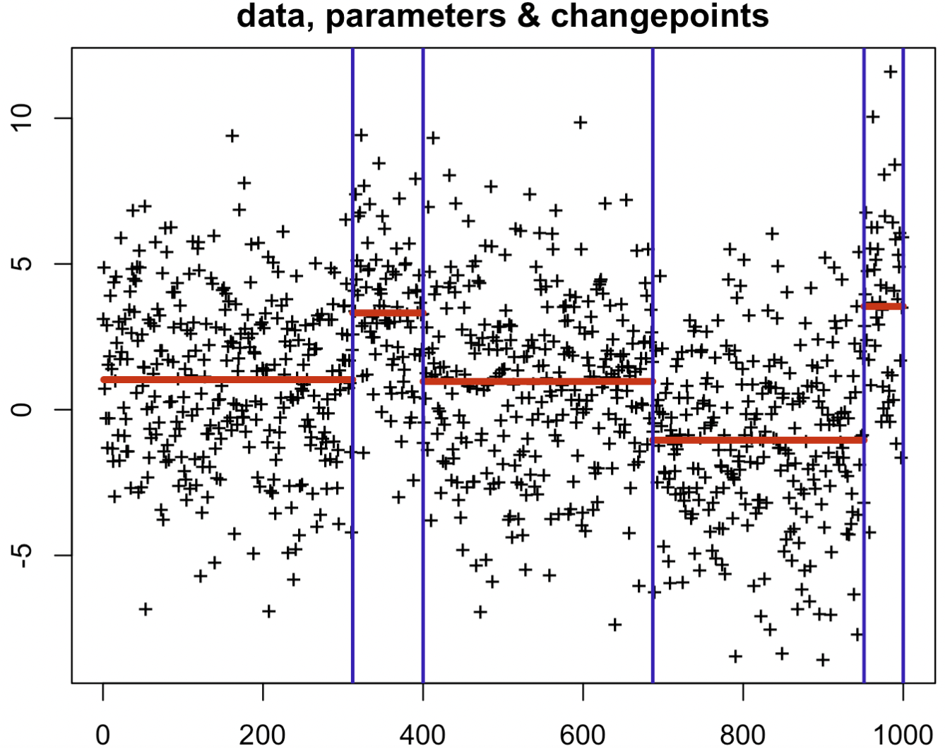
R> set.seed(75)R> n <- 1000R> myData <- dataGenerator(n, c(0.1, 0.3, 0.5, 0.8, 1),+ c(1, 2, 1, 3, 1), sigma = 1)This data has segments, with the end of segments at relative positions , , , and along the data points; and with segment means being respectively and .
R> set.seed(75)R> n <- 1000R> myData <- dataGenerator(n, c(0.1, 0.3, 0.5, 0.8, 1),+ c(1, 2, 1, 3, 1), sigma = 1)R> myGraph <- graph(penalty = 2 * log(n), type = "updown")R> gfpop(data = myData, mygraph = myGraph, type = "mean")
$changepoints[1] 108 295 500 800 1000$states[1] "Dw" "Up" "Dw" "Up" "Dw"$forced[1] FALSE FALSE FALSE FALSE$parameters[1] 1.044920 2.047202 1.017550 2.916826 1.030938$globalCost[1] 963.0278attr(,"class")[1] "gfpop" "mean"The call to the Πgfpop function requires specifying the data, the graph that encapsulates the changepoint model, and the type of loss function. Here Πtype = ”mean” specifies the use of the L2 or biweight loss.
The response contains four vectors. A vector Πchangepoints contains the last index of each segment, a vector Πstates gives the nodes in which lie the successive parameter values of the Πparameters vector. The vector Πforced is a vector of booleans of size ’number of segments - 1’ with entry ΠTRUE when the transition between two states (nodes) has been forced. The ΠglobalCost is the non-penalized cost.
Gaussian Robust biweight model with an up-down graph.
Below we illustrate the use of the biweight loss on data where of the data points are outliers. We shift these data by using function Πrbinom (4th line of code below). We use the biweight loss with and an Πupdown graph with a difference of at least between consecutive means.
R> n <- 1000R> chgtpt <- c(0.1, 0.3, 0.5, 0.8, 1)R> myData <- dataGenerator(n, chgtpt, c(0, 1, 0, 1, 0), sigma = 1)R> myData <- myData + 5 * rbinom(n, 1, 0.05) - 5 * rbinom(n, 1, 0.05)R> beta <- 2 * log(n)R> myGraph <- graph(+ Edge("Dw", "Up", type = "up", penalty = beta, gap = 1, K = 3),+ Edge("Up", "Dw", type = "down", penalty = beta, gap = 1, K = 3),+ Edge("Dw", "Dw", type = "null", K = 3),+ Edge("Up", "Up", type = "null", K = 3),+ StartEnd(start = "Dw", end = "Dw"))R> gfpop(data = myData, mygraph = myGraph, type = "mean")
$changepoints[1] 102 311 500 806 1000$states[1] "Dw" "Up" "Dw" "Up" "Dw"$forced[1] TRUE FALSE FALSE FALSE$parameters[1] -0.02296768 0.97703232 -0.03434534 1.00246359 -0.03334062$globalCost[1] 1097.364attr(,"class")[1] "gfpop" "mean"The difference between this graph and the one for the previous example is the specification ΠK = 3 for each edge. This enforces the use of the biweight loss (with ) as opposed to the L2 loss.
Poisson model with isotonic up graph.
We provide an example with a Lin-log cost decomposition with Poisson data constrained to up changes, with the mean at least a doubling at each change.
R> n <- 1000R> chgtpt <- c(0.1, 0.3, 0.5, 0.8, 1)R> myData <- dataGenerator(n, chgtpt, c(1, 3, 5, 7, 12), type = "poisson")R> beta <- 2 * log(n)R> myGraph <- graph(type = "isotonic", gap = 2)R> gfpop(data = myData, mygraph = myGraph, type = "poisson")
$changepoints[1] 2 99 297 796 1000$states[1] "Iso" "Iso" "Iso" "Iso" "Iso"$forced[1] TRUE FALSE TRUE TRUE$parameters[1] 0.4693878 0.9387755 2.9840954 5.9681909 11.9363817$globalCost[1] -5832.845attr(,"class")[1] "gfpop" "poisson"The use of Poisson loss is enforced by Πtype = ”poisson” in the call to Πgfpop. The graph that describes our change-point model is the default one for isotonic changes, but with the additional constraint on means at least doubling being specified by Πgap = 2.
Negative binomial model with 3-segment graph.
The parameters to find are probabilities and we restrict the inference to 3 segments. The optional parameter Πall.null.edges in graph function automatically generates Πnull edges for all nodes.
R> myGraph <- graph(+ Edge("1", "2", type = "std", penalty = 0),+ Edge("2", "3", type = "std", penalty = 0),+ StartEnd(start = "1", end = "3"),+ all.null.edges = TRUE)R> myData <- dataGenerator(n = 1000, changepoints = c(0.3,0.7,1),+ parameters = c(0.2,0.25,0.3), type = "negbin")R> gfpop(myData, myGraph, type = "negbin")
$changepoints[1] 300 714 1000$states[1] "1" "2" "3"$forced[1] FALSE FALSE$parameters[1] 0.2117808 0.2652162 0.3212748$globalCost[1] 2193.216attr(,"class")[1] "gfpop" "negbin"
Each data-point can be weighted using parameter Πweights in Πgfpop function. It can be useful to gather consecutive identical values for count data time-series in order to speed-up the change-point analysis Cleynen et al. 2014.
4.3 Some additional useful functions in gfpop
Standard deviation estimation.
For many real-data-sets examples, we are obliged to estimate the standard deviation from the observed data. This value is then used to normalize the data or to be included in edge penalties. The ΠsdDiff() returns such an estimation with the default HALL method (Hall et al. 1990) well suited for time series with change-points.
A plotting function.
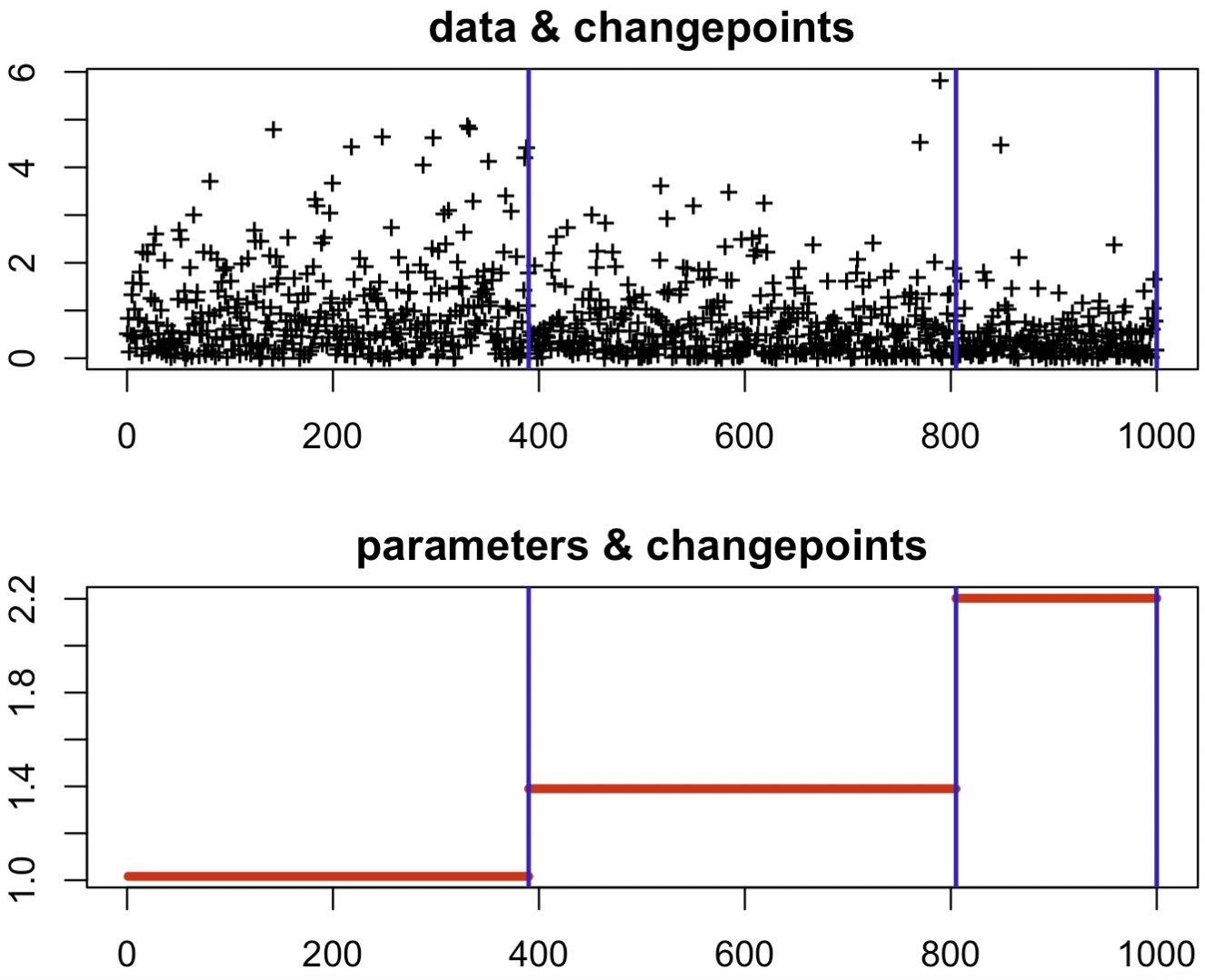
We defined a plotting function Πplot(), which shows data-points and the results of the Πgfpop() function by using inferred segment parameters and change-points. The user can plot the result in two graphs or only one for Πmean and Πpoisson types (see parameter Πmultiple) and has to explicitly use the Πdata parameter as in following examples.
Example 1:
R> set.seed(86)R> myData <- dataGenerator(1000, c(0.3, 0.4, 0.7, 0.95, 1),+ c(1, 3, 1, -1, 4), "mean", sigma = 3)R> s <- sdDiff(myData)R> g <- gfpop(myData,+ graph(type = "relevant", gap = 0.5, penalty = 2 * s ^ 2 * log(1000)),+ type = "mean")R> plot(x = g, data = myData, multiple = FALSE)
Example 2:
R> set.seed(86)R> myData <- dataGenerator(1000, c(0.4, 0.8, 1), c(1, 1.3, 2.3), "exp")R> s <- sdDiff(myData)R> g <- gfpop(myData, type = "exp",+ graph(type = "isotonic", penalty = 2 * s ^ 2 * log(1000)))R> plot(x = g, data = myData, multiple = TRUE)
5 Modeling real data with graph-constrained models
In this section we illustrate the use of our package on several real datasets. For each application we illustrate several possible sets of constraints and briefly discuss their relative advantages.
5.1 Gaussian model for DNA copy number data
We consider DNA copy number data, which are biological measurements that characterize the number of chromosomes in cell samples. Abrupt changes along chromosomes in these data are important indicators of severity in cancers such as neuroblastoma (Schleiermacher et al. 2010). The non-constrained Gaussian segmentation model has been shown to have state-of-the-art change-point detection accuracy in these data (Hocking et al. 2013).
However, in some high-density copy number data sets, this model incorrectly detects small changes in mean which are not relevant (Hocking and Rigaill 2012). One such data set is shown in Figure 11, which also has positive and negative labels from an expert genomic scientist that indicated regions with (1breakpoint) or without (0breakpoints) relevant change-points. We used these labels to quantify the accuracy of three unconstrained Gaussian change-point models with several different penalties .

- •
The model with 13 segments predicts a change-point in each positive label (0/6 false negatives), but predicts one change-point in the negative label (1 false positive), for a total of 1 incorrectly predicted label. (bottom panel)
- •
The model with 7 segments predicts a change-point in four positive labels (2/6 false negatives), and also predicts the false positive change-point in the negative label, for a total of 3 incorrectly predicted labels. (second panel from bottom)
- •
The model with 3 segments predicts a change-point in only two positive labels (4/6 false negatives), and predicts no change-point in the negative label (0/1 false positive), for a total of 4 incorrectly predicted labels. (second panel from top)
We computed all non-constrained Gaussian models from 1 to 20 segments for these data, and none of them were able to provide change-point predictions that perfectly match the expert-provided labels (each model had at least one false positive or false negative). It is thus problematic to use the unconstrained change-point model in this context, because none of the unconstrained models achieve zero label errors.
To solve this problem we propose a graph (Figure 11, top graph) which enforces only “relevant” change-points , for some relevant threshold . For the DNA copy number data set, we set and choose such that the algorithm returns 13 segments (Figure 11, top panel with blue model). The proposed model predicts a change-point in each of the positive labels, but does not predict a change-point in the negative label. The proposed graph-constrained change-point model is therefore able to predict change-points that perfectly match the expert-provided labels. If overfitting is a concern with this procedure, we can consider using the two labels in the last region as a test set (105.9-106.5 mega bases), and the other labels as a train set. In that case we chose the penalty with minimal errors with respect to the train set labels, and we observed that the test set label error was also minimized.
5.2 Gaussian multi-modal regression for neuro spike train data
The so-called AR1 change-point model, where the mean decreases exponentially within each segment has been proposed for detecting spikes in calcium imaging data from neuroscience (Jewell et al. 2020). We fit this model to one calcium imaging data set (Figure 12, Right top) and observed that it is difficult to find a parameter that detects both labeled spikes. Red rectangles in Figure 12 indicate labels provided by an electrophysiological method which is taken as ground-truth in order to emphasize the qualitative difference between the two algorithms. Part of the difficulty of the AR1 model is the fact that there are two parameters to tune, the penalty and also the exponential decay parameter . It is more difficult to tune two parameters using grid search because of its quadratic time complexity. Another issues is that a visual inspection of the data suggests that the rate of decay of the mean between spikes may not be constant as assumed by the AR1 model.
We therefore propose a new multi-modal regression model (Isotonic up - Isotonic down graph shown in Figure 12, left) with only one parameter, the penalty . We can view this model as detecting modes in the data. Each mode consists of a period before-hand where the mean increases followed by a period where then mean decreases. The period where the mean increases can be interpreted as a period of time where a spike occurs, with the periods where the mean decreases modeling the decay in the data after the spike end. The number of detected spikes is equal to the number of regions where the mean increases, and is controlled by the penalty . We observed that it is easy to find a penalty which detects both labeled spikes. Overall these results indicate that the proposed multi-modal regression model (Isotonic up - Isotonic down) is promising for spike detection in calcium imaging data. We leave a more extensive quantitative comparison to future work.

5.3 Gaussian nine-state model for electrocardiogram data
In the context of monitoring hospital patients with heart problems, electrocardiogram (ECG) analysis is one of the most common non-invasive techniques for diagnosing several heart arrhythmia (Afghah et al. 2015).
A preliminary and fundamental step in ECG analysis is the detection of the QRS complex that leads to detecting the heartbeat and classifying the rhythms Mousavi and Afghah 2019.
Here, we utilize the proposed change-point detection method to locate the QRS complex in ECG waveforms. The ECG signals used in this study are extracted from the publicly available Physionet Challenge 2015 database PhysioNet 2015; Clifford et al. 2016 that includes measurements for three physiological signals (including ECG) for 750 patients. The resolution and frequency of each signal are 12bit and 250 Hz, respectively. Also, each signal has been filtered by a finite impulse response (FIR) band pass [0.05 to 40Hz] and mains notch filters.
Pan-Tompkins algorithm is one of the most common segmentation methods used for ECG analysis (Pan and Tompkins 1985; Agostinelli et al. 2017). This method uses a patient-specific threshold-based approach for real-time detection of the QRS complex in ECG signals, which represents the ventricular depolarization. In this algorithm, after a pre-processing step by a band-pass filter, the signal is passed through differentiation and squaring blocks to determine and amplify the slope of QRS, followed by a moving window integration step with an adaptive set of thresholds to determine the peaks. The detection thresholds are learned at the beginning of the algorithm and are calibrated periodically to follow the variations of the ECG signal.
Figure 14 (top) shows four seconds of ECG data for which we predicted the QRS complex using the well-known Pan-Tompkins method. The peak of each heartbeat should be predicted as R, but the algorithm incorrectly predicts S in two cases. In contrast the peak is correctly classified as R (bottom) using our proposed model with nine states (see Figure 13), which were determined using prior knowledge about the expected sequence of changes. In this model, the QRS complex is modeled by an up-spike followed by a down spike with the maximum amplitude difference related to adjacent spikes. The graph model considers a vertex for each main waveform(i.e., P, Q, R, S, T) as well as three baselines, which are intermediate states (Fotoohinasab et al. 2021).

6 Isotonic regression using constraint graph with robust loss
Our package can be used with robust loss functions which have been shown to be useful in the presence of outliers (Fearnhead and Rigaill 2019) and in particular in the context of isotonic regression (Bach 2018). Here we illustrate this on simulations inspired by those of Bach 2018 (see Figure 15 with corrupted data). We compare our package using the isotonic model described in Figure 5 with several implementations of the PAVA algorithm (Best and Chakravarti 1990; De Leeuw et al. 2010).
Relative to the very fast PAVA, our dynamic programming algorithm is slower. However, PAVA only works for the square loss and the non-penalized model (maximum number of changes). In contrast, Πgfpop() can handle non-convex losses (such as the biweight loss) and can include a positive penalty in order to reduce the number of changes.
6.1 Parametrization
gfpop.
In all simulations we used gfpop with the graph of Figure 5 and a quadratic (L2) or a biweight loss (bw). We considered two different values for the penalty : and , with the true variance. Thus, we have 4 different algorithms of the Πgfpop() function: Πgfpop1 (, ), Πgfpop2 (, ), Πgfpop3 (, ) and Πgfpop4 (, ).
Competitors.
We compared the output of gfpop with those of 2 isotonic regression package functions:
- •
Πisoreg() function of the stats package which is based on the very fast Pool adjacent violators algorithm for the loss (Best and Chakravarti 1990);
- •
Πreg Π1d() function developed in package UniIsoRegression which solves the isotonic regression problem for the and losses (Stout 2008).
We also include a simple linear regression approach (Πlm() function of the stats package) as a reference. In total we have 4 competitors (Πlm(), Πisoreg(), Πreg Π1d() with the and losses).
6.2 Simulated data
We focused on two types of increasing signals:
- linear:
-
as in Bach 2018 we consider linearly increasing time series with a signal
- step-wise:
-
as our package is devoted to change-point inference we also consider a step-wise increasing series (with steps) with a signal
We consider three ways to corrupt the data.
- Gaussian noise:
-
here we simply add a Gaussian noise, with a variance to the signal (i.e., ).
- Student noise:
-
we also considered a Student noise with a degree of freedom equal to .
- Corrupted noise:
-
in the most difficult scenario, suggested by Bach 2018, we randomly select a proportion of data-points and multiply them by and then add a Gaussian noise, i.e., , where is a Bernoulli trial with probability to get and probability to get . We fix for all simulations.
In total we have 6 scenarios (2 signals and 3 ways to corrupt the data). In Figure 15 we illustrate those 6 scenarios with and , which is an example of time series used in following simulations.

Criteria.
To assess the quality of the results, we compute the Mean-Squared Error (MSE) as well as the ability to recover the true number of changes when there are changes in the data in the step-wise scenario.
6.3 A simple illustration
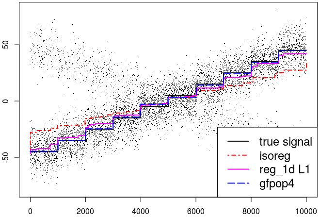
We illustrate our results on a step-wise increasing signal with corrupted data. In Figure 16, we represent the data and the results of various approaches. We see that using a biweight loss our package in blue is closer to the true signal in black than other approaches.
In Appendix we considered Monte-Carlo simulations to confirm this result: see Section D.1 for the linear increasing scenario and Section D.2 for the step-wise increasing scenario. As expected, recovering the true number of changes with corrupted data with also a small MSE is a challenging task for all methods excepted for Πgfpop4() using a robust loss, a positive penalty and the isotonic constraint graph. The R code of these simulations can be found on the Github page https://github.com/vrunge/gfpop/tree/master/simulations.
7 Conclusion
In this paper we described the gfpop package, which provides a generalized version of an algorithm recently proposed by Hocking et al. 2020 for penalized maximum likelihood inference of constrained multiple change-point models. The gfpop package implements the algorithm in a generic manner in R/C++ and allows the user to specify the constraint graph in R code. We explained how these constrained multiple change-point models can also be seen as constrained continuous state space HMM. gfpop allows one to encode modeling assumptions on the type of changes using a graph of states and constraints. We illustrated the use of gfpop on isotonic simulations and several applications in biology.
For a number of graphs the algorithm runs in a matter of seconds or minutes for data-points. While gfpop can be used to fit simple change-point models, such as the standard change in mean in Gaussian data, it is slower than fpop which implements functional programming specifically for that model: For example, for points with no change fpop runs in seconds and gfpop in seconds. This is because the gfpop is coded in a more generic manner, as it handles constraints and various losses. As we illustrated with numerous examples, the advantage of gfpop is that it allows one to include constraints and/or unconventional losses, and thus fit a range of change-point models that cannot be fit by other generic software.
Future Work.
For future work we are interested to explore generalizations which allow time-dependent constraints. As mentioned in Section 2.2 our implementation only allows inference in models that can be represented by a collapsed graph with transitions that are valid for all time points. We are interested in exploring new frameworks for defining which transitions and/or states are feasible at which time points, in order to efficiently support inference in models such as Labeled Optimal Partitioning (Dylan Hocking and Srivastava 2020). There are a number of other extensions of gfpop that are possible, including allowing local fluctuations in the parameter between change-points and modeling auto-correlated noise – these can be both be incorporated using ideas from Romano et al. 2021. Another extension would be to consider the detection of change-points in trees as proposed in chapter three of the Ph.D. thesis of Thépaut 2019. Furthermore, the underlying Πgfpop algorithm is sequential and thus can be adapted to allow for online change-point detection.
References
- Hocking et al. [2020] Toby Dylan Hocking, Guillem Rigaill, Paul Fearnhead, and Guillaume Bourque. Constrained dynamic programming and supervised penalty learning algorithms for peak detection in genomic data. Journal of Machine Learning Research, 21(87):1–40, 2020.
- Truong et al. [2020] Charles Truong, Laurent Oudre, and Nicolas Vayatis. Selective review of offline change point detection methods. Signal Processing, 167:107299, 2020.
- Scott and Knott [1974] Alastair J Scott and M Knott. A cluster analysis method for grouping means in the analysis of variance. Biometrics, 30(3):507–512, 1974.
- Olshen et al. [2004] Adam B Olshen, ES Venkatraman, Robert Lucito, and Michael Wigler. Circular binary segmentation for the analysis of array-based DNA copy number data. Biostatistics, 5(4):557–572, 2004.
- Fryzlewicz [2014] Piotr Fryzlewicz. Wild binary segmentation for multiple change-point detection. Annals of Statistics, 42(6):2243–2281, 2014.
- Frick et al. [2014] Klaus Frick, Axel Munk, and Hannes Sieling. Multiscale change point inference. Journal of the Royal Statistical Society B, 76(3):495–580, 2014.
- Eichinger and Kirch [2018] Birte Eichinger and Claudia Kirch. A MOSUM procedure for the estimation of multiple random change points. Bernoulli, 24(1):526–564, 2018.
- Baranowski and Fryzlewicz [2014] R Baranowski and P Fryzlewicz. wbs: Wild Binary Segmentation for multiple change-point detection, 2014. R package version 1.4.
- Baranowski et al. [2019] Rafal Baranowski, Yining Chen, and Piotr Fryzlewicz. Narrowest-over-threshold detection of multiple change points and change-point-like features. Journal of the Royal Statistical Society B, 81(3):649–672, 2019.
- Anastasiou et al. [2020] Andreas Anastasiou, Yining Chen, Haeran Cho, and Piotr Fryzlewicz. breakfast: Methods for fast multiple change-point detection and estimation, 2020. URL https://CRAN.R-project.org/package=breakfast. R package version 2.1.
- Pein et al. [2020] Florian Pein, Thomas Hotz, Hannes Sieling, and Timo Aspelmeier. stepR: Multiscale change-point inference, 2020. URL https://CRAN.R-project.org/package=stepR. R package version 2.1-1.
- Meier et al. [2021] Alexander Meier, Claudia Kirch, and Haeran Cho. mosum: A package for moving sums in change point analysis. Journal of Statistical Software, to appear, 2021.
- Fearnhead and Rigaill [2020] Paul Fearnhead and Guillem Rigaill. Relating and comparing methods for detecting changes in mean. Stat, 9(1):e291, 2020.
- Auger and Lawrence [1989] Ivan E Auger and Charles E Lawrence. Algorithms for the optimal identification of segment neighborhoods. Bulletin of Mathematical Biology, 51(1):39–54, 1989.
- Jackson et al. [2005] Brad Jackson, Jeffrey D Scargle, David Barnes, Sundararajan Arabhi, Alina Alt, Peter Gioumousis, Elyus Gwin, Paungkaew Sangtrakulcharoen, Linda Tan, and Tun Tao Tsai. An algorithm for optimal partitioning of data on an interval. IEEE Signal Processing Letters, 12(2):105–108, 2005.
- Killick et al. [2012] Rebecca Killick, Paul Fearnhead, and Idris A Eckley. Optimal detection of changepoints with a linear computational cost. Journal of the American Statistical Association, 107(500):1590–1598, 2012.
- Killick and Eckley [2014] Rebecca Killick and Idris A Eckley. changepoint: An R package for changepoint analysis. Journal of Statistical Software, 58(3):1–19, 2014.
- Haynes et al. [2016] K Haynes, R Killick, P Fearnhead, I A Eckley, and D Grose. changepoint.np: Methods for nonparametric changepoint detection, 2016. URL https://CRAN.R-project.org/package=changepoint.np.
- Johnson [2013] Nicholas A. Johnson. A Dynamic Programming Algorithm for the Fused Lasso and L0-Segmentation. Journal of Computational and Graphical Statistics, 22(2):246–260, 2013.
- Rigaill [2015] Guillem Rigaill. A pruned dynamic programming algorithm to recover the best segmentations with 1 to k_max change-points. Journal de la Société Française de Statistique, 156(4):180–205, 2015.
- Maidstone et al. [2017] Robert Maidstone, Toby Hocking, Guillem Rigaill, and Paul Fearnhead. On optimal multiple changepoint algorithms for large data. Statistics and Computing, 27(2):519–533, 2017.
- Cleynen et al. [2014] Alice Cleynen, Michel Koskas, Emilie Lebarbier, Guillem Rigaill, and Stéphane Robin. Segmentor3IsBack: an R package for the fast and exact segmentation of seq-data. Algorithms for Molecular Biology, 9(1):1–11, 2014.
- Pierre-Jean et al. [2019] Morgane Pierre-Jean, Guillem Rigaill, and Pierre Neuvial. jointseg: Joint segmentation of multivariate (copy number) signals, 2019. URL https://CRAN.R-project.org/package=jointseg. R package version 1.0.2.
- Hocking et al. [2015] Toby Hocking, Guillem Rigaill, and Guillaume Bourque. PeakSeg: constrained optimal segmentation and supervised penalty learning for peak detection in count data. In International Conference on Machine Learning, pages 324–332. PMLR, 2015.
- Hocking et al. [2022] Toby Dylan Hocking, Guillem Rigaill, Paul Fearnhead, and Guillaume Bourque. Generalized functional pruning optimal partitioning (gfpop) for constrained changepoint detection in genomic data. Journal of Statistical Software, 101(10):1–31, 2022. doi: 10.18637/jss.v101.i10. URL https://www.jstatsoft.org/index.php/jss/article/view/v101i10.
- Hocking and Bourque [2020] Toby Dylan Hocking and Guillaume Bourque. Machine learning algorithms for simultaneous supervised detection of peaks in multiple samples and cell types. In Proc. Pacific Symposium on Biocomputing, volume 25, pages 367–378, 2020.
- Jewell et al. [2020] Sean Jewell, Toby Dylan Hocking, Paul Fearnhead, and Daniela Witten. Fast nonconvex deconvolution of calcium imaging data. Biostatistics, 21(4):709–726, 2020.
- Barlow et al. [1972] Richard E Barlow, David J Bartholomew, James M Bremner, and H Daniel Brunk. Statistical inference under order restrictions: The theory and application of isotonic regression. Technical report, 1972. Defense Technology Information Centre, Report AD0751311.
- Best and Chakravarti [1990] Michael J Best and Nilotpal Chakravarti. Active set algorithms for isotonic regression; a unifying framework. Mathematical Programming, 47(1-3):425–439, 1990.
- Gao et al. [2020] Chao Gao, Fang Han, and Cun-Hui Zhang. On estimation of isotonic piecewise constant signals. Annals of Statistics, 48(2):629–654, 2020.
- De Leeuw et al. [2010] Jan De Leeuw, Kurt Hornik, and Patrick Mair. Isotone optimization in r: pool-adjacent-violators algorithm (pava) and active set methods. Journal of statistical software, 32:1–24, 2010.
- Stout [2008] Quentin F Stout. Unimodal regression via prefix isotonic regression. Computational Statistics and Data Analysis, 53(2):289–297, 2008.
- Fearnhead and Rigaill [2019] Paul Fearnhead and Guillem Rigaill. Changepoint detection in the presence of outliers. Journal of the American Statistical Association, 114(525):169–183, 2019.
- Bach [2018] Francis Bach. Efficient algorithms for non-convex isotonic regression through submodular optimization. In NIPS’18: Proceedings of the 32nd International Conference on Neural Information Processing Systems, pages 1–10, 2018.
- Fisch et al. [2018] Alexander Tristan Maximilian Fisch, Idris Arthur Eckley, and Paul Fearnhead. A linear time method for the detection of point and collective anomalies, 2018. arXiv:1806.01947.
- Dette and Wied [2016] Holger Dette and Dominik Wied. Detecting relevant changes in time series models. Journal of the Royal Statistical Society B, 78(2):371–394, 2016.
- Picard et al. [2005] Franck Picard, Stephane Robin, Marc Lavielle, Christian Vaisse, and Jean-Jacques Daudin. A statistical approach for array CGH data analysis. BMC bioinformatics, 6(1):27, 2005.
- Yao and Au [1989] Yi-Ching Yao and Siu-Tong Au. Least-squares estimation of a step function. Sankhyā: The Indian Journal of Statistics, Series A, 51(3):370–381, 1989.
- Zhang and Siegmund [2007] Nancy R Zhang and David O Siegmund. A modified bayes information criterion with applications to the analysis of comparative genomic hybridization data. Biometrics, 63(1):22–32, 2007.
- Lebarbier [2005] Émilie Lebarbier. Detecting multiple change-points in the mean of gaussian process by model selection. Signal processing, 85(4):717–736, 2005.
- Baraud et al. [2009] Yannick Baraud, Christophe Giraud, and Sylvie Huet. Gaussian model selection with an unknown variance. The Annals of Statistics, 37(2):630–672, 2009.
- Haynes et al. [2017] Kaylea Haynes, Idris A Eckley, and Paul Fearnhead. Efficient penalty search for multiple changepoint problems. Journal of Computational and Graphical Statistics, 26(1):134–143, 2017.
- Rigaill et al. [2013] Guillem Rigaill, Toby D Hocking, Jean-Philippe Vert, and Francis Bach. Learning sparse penalties for change-point detection using max margin interval regression. In Proc. 30th ICML, pages 172–180, 2013.
- Hall et al. [1990] Peter Hall, JW Kay, and DM Titterinton. Asymptotically optimal difference-based estimation of variance in nonparametric regression. Biometrika, 77(3):521–528, 1990.
- Schleiermacher et al. [2010] Gudrun Schleiermacher, Isabelle Janoueix-Lerosey, Agnès Ribeiro, Jerzy Klijanienko, Jérôme Couturier, Gaëlle Pierron, Véronique Mosseri, Alexander Valent, Nathalie Auger, Dominique Plantaz, Hervé Rubie, Dominique Valteau-Couanet, Franck Bourdeaut, Valérie Combaret, Christophe Bergeron, Jean Michon, and Olivier Delattre. Accumulation of segmental alterations determines progression in neuroblastoma. Journal of Clinical Oncology, 28(19):3122–3130, 2010. doi: 10.1200/JCO.2009.26.7955. PMID: 20516441.
- Hocking et al. [2013] Toby Dylan Hocking, Gudrun Schleiermacher, Isabelle Janoueix-Lerosey, Valentina Boeva, Julie Cappo, Oliver Delattre, Francis Bach, and Jean-Philippe Vert. Learning smoothing models of copy number profiles using breakpoint annotations. BMC Bioinformatics, 14(164), May 2013.
- Hocking and Rigaill [2012] T. D. Hocking and G. J. Rigaill. SegAnnot: an R package for fast segmentation of annotated piecewise constant signals. HAL technical report 00759129, 2012.
- Afghah et al. [2015] F. Afghah, A. Razi, and K. Najarian. A shapley value solution to game theoretic-based feature reduction in false alarm detection. Neural Information Processing Systems (NIPS), Workshop on Machine Learning in Healthcare, arXiv:1512.01680, Dec. 2015.
- Mousavi and Afghah [2019] S. Mousavi and F. Afghah. Inter- and intra- patient ecg heartbeat classification for arrhythmia detection: A sequence to sequence deep learning approach. In ICASSP 2019 - 2019 IEEE International Conference on Acoustics, Speech and Signal Processing (ICASSP), pages 1308–1312, 2019. doi: 10.1109/ICASSP.2019.8683140.
- PhysioNet [2015] PhysioNet. Reducing false arrhythmia alarms in the ICU, 2015. URL http://www.physionet.org/challenge/2015/. accessed July 28, 2016.
- Clifford et al. [2016] G. Clifford, I. Silva, B. Moody, Q. Li, D. Kella, A. Chahin, T. Kooistra, D. Perry, and R. Mark. False alarm reduction in critical care. Physiological Measurement, 37(8):5–23, 2016.
- Pan and Tompkins [1985] J. Pan and W. J. Tompkins. A real-time QRS detection algorithm. IEEE Transactions on Biomedical Engineering, BME-32(3):230–236, March 1985. ISSN 0018-9294. doi: 10.1109/TBME.1985.325532.
- Agostinelli et al. [2017] A. Agostinelli, I. Marcantoni, E. Moretti, A. Sbrollini, S. Fioretti, F. Di Nardo, and L. Burattini. Noninvasive fetal electrocardiography part i: Pan-tompkins’ algorithm adaptation to fetal r-peak identification. The Open Biomedical Engineering Journal, 11:17–24, 2017.
- Fotoohinasab et al. [2021] Atiyeh Fotoohinasab, Toby Hocking, and Fatemeh Afghah. A greedy graph search algorithm based on changepoint analysis for automatic qrs complex detection. Computers in Biology and Medicine, 130:104208, 2021.
- Dylan Hocking and Srivastava [2020] Toby Dylan Hocking and Anuraag Srivastava. Labeled optimal partitioning. arXiv e-prints, pages arXiv–2006, 2020.
- Romano et al. [2021] Gaetano Romano, Guillem Rigaill, Vincent Runge, and Paul Fearnhead. Detecting abrupt changes in the presence of local fluctuations and autocorrelated noise. Journal of the American Statistical Association, pages 1–16, 2021.
- Thépaut [2019] Solène Thépaut. Problèmes de clustering liés à la synchronie en écologie : estimation de rang effectif et détection de ruptures sur les arbres. PhD thesis, 2019. URL http://www.theses.fr/2019SACLS477. Thèse de doctorat dirigée par Giraud, Christophe Mathématiques aux interfaces Université Paris-Saclay (ComUE) 2019.
Appendix A Some other graphs
Here are three graphs for models discussed in the main part of the paper.
Below we provide a few other constraint models and their graphs.
- •
- •
(Up - Down with at least two data-points) If one wants to detect peaks and is certain that segments are at least of length 2 it suffices to add two waiting states in the Up - Down graph. The graph of this model is given Figure 21.
- •
(Up - Isotonic Down) In the pulse detection example (Up - Exponentially Down model in Figure 7) if one is not sure of the exponential decrease it could make sense to consider an isotonic decrease. For this it suffices to consider two states . Compared to the Up - Down model, described earlier, we add an additional transition from to with the constraint . The graph of this model is given in Figure 22.
- •
(Isotonic Up - Isotonic Down) In the previous model one considers a sharp transition up. It might make sense to consider an isotonic increase. For this it suffices to add an edge from to in the previous model. Only transitions from to and to are penalized. The graph of this model is given in Figure 23.
Appendix B Update-rule proof
We name the path and vector realizing the best cost , defined in Equation 1, and . We call the corresponding vector of states. We have , and
We will first show that
(Proof) Restricting the path and the vector to their first elements, by definition of we have Also, given that a move from parameter to is a valid transition from state to and by the definition of , we have
We will now proceed by contradiction. Let us assume that . We name the path and vector realizing the and Extending this path and vector to with and we get a better cost than for which is a contradiction.
So we have
and considering all possible states at time we get the update-rule.
Appendix C Backtracking
After running the Viterbi-like algorithm with update-rule 2, we need a backward procedure called backtracking to return the optimal change-point vector. First, we recover using Algorithm 1 the optimal vector of states and vector of means . We then find the best change-point vector with Algorithm 2. The basic idea of Algorithm 1 is that if we knew and we could recover first and then taking the argmin of the update-rule (see lines 8 and 9 of Algorithm 1).
The obtained vectors and are simplified removing repetitions of consecutive identical states or values: i.e., and for (including the case of exponential decay with parameter and if no decay). In that case, the index is an element of the change-point vector and its associated segment parameter. The vector of change-points can be built by a linear-in-time procedure described in Algorithm 2.
Notice that is the Πchangepoints vector returned by the Πgfpop() function. Restricting and vectors to positions in , these vectors are respectively the Πstates and the Πparameters vectors.
Appendix D Simulation results for isotonic regression
D.1 Linear signal
We simulate linearly increasing time series and compute the mean of the MSE for each noise structure. The results are in Table 1. We highlight in bold the two best results in each row and also give the standard deviation (SD).
In the Gaussian case the isotonic regression and Πgfpop1 (with and ) are better. For the Student and for the Corrupted scenarios the robust biweight loss with is performing better in terms of MSE. Note that it is however much slower than PAVA. Including a penalty for change-points () deteriorates the results. This make sense as there are in fact no change-points in the data.
| Isolinear | linear | Πisoreg | Πreg Π1d | Πreg Π1d | Πgfpop1 | Πgfpop2 | Πgfpop3 | Πgfpop4 |
| simulations | fit | |||||||
| Gauss | ||||||||
| MSE | 0.0190 | 0.714 | 0.712 | 1.08 | 0.826 | 0.931 | 2.60 | 3.10 |
| (SD) | (0.020) | (0.098) | (0.098) | (0.17) | (0.15) | (0.13) | (0.27) | (0.30) |
| Student | ||||||||
| MSE | 0.0185 | 0.683 | 0.681 | 0.550 | 0.780 | 0.555 | 2.56 | 2.57 |
| (SD) | (0.19) | (0.12) | (0.12) | (0.077) | (0.17) | (0.076) | (0.24) | (0.22) |
| Corrupted | ||||||||
| MSE | 299 | 298 | 298 | 28.7 | 294 | 4.05 | 301 | 7.23 |
| (SD) | (9.1) | (8.8) | (8.8) | (2.2) | (11) | (0.63) | (8.9) | (0.89) |
D.2 Iso-step signal
We simulate step-wise increasing time series with segments and compute the mean of the MSE for each noise structure. The results are in Table 2. We highlight in bold the two best results in each row and also give the standard deviation (SD).
In Gaussian and Student cases the penalized algorithms Πgfpop3 and Πgfpop4 with are better. For the corrupted scenario, we need the robust loss of algorithms Πgfpop2 and Πgfpop4 to get a much better MSE than other approaches. To confirm the benefit of using a penalized approach in Student case, we plot the distribution of the MSE for the five best algorithms in Figure 24.
| Iso-step | linear | Πisoreg | Πreg Π1d | Πreg Π1d | Πgfpop1 | Πgfpop2 | Πgfpop3 | Πgfpop4 |
| simulations | fit | |||||||
| Gauss | ||||||||
| MSE | 8.27 | 0.635 | 0.632 | 1.34 | 1.21 | 0.842 | 0.358 | 0.470 |
| (SD) | (0.022) | (0.11) | (0.10) | (0.30) | (0.78) | (0.16) | (0.12) | (0.17) |
| Student | ||||||||
| MSE | 8.27 | 0.571 | 0.569 | 0.564 | 1.09 | 0.439 | 0.301 | 0.201 |
| (SD) | (0.024) | (0.15) | (0.15) | (0.14) | (1.0) | (0.13) | (0.15) | (0.073) |
| Corrupted | ||||||||
| MSE | 304 | 300 | 300 | 30.1 | 297 | 3.57 | 301 | 3.17 |
| (SD) | (7.6) | (7.3) | (7.2) | (3.5) | (11) | (0.53) | (7.3) | (0.59) |

We also compare the ability of the different methods to estimate the number of steps. The average number of steps over simulations is reported in Table 3. Only the penalized algorithms are able to recover the true number of steps (). The choice of a good penalty in isotonic simulations is an area of ongoing research in statistics [Gao et al. 2020].
| Iso-step | Πisoreg | Πreg Π1d | Πreg Π1d | Πgfpop1 | Πgfpop2 | Πgfpop3 | Πgfpop4 |
|---|---|---|---|---|---|---|---|
| simulations | |||||||
| Gauss | |||||||
| 66.8 | 66.7 | 59.0 | 69.1 | 66.7 | 10.0 | 10.0 | |
| (SD) | (7.0) | (7.0) | (6.0) | (7.6) | (7.6) | (0) | (0) |
| Student | |||||||
| 69.6 | 69.4 | 63.2 | 70.5 | 71.0 | 10.1 | 10.0 | |
| (SD) | (7.2) | (7.2) | (6.8) | (7.9) | (8.2) | (0.24) | (0) |
| Corrupted | |||||||
| 40.9 | 40.8 | 47.8 | 41.5 | 61.6 | 11.2 | 10.0 | |
| (SD) | (5.2) | (5.2) | (5.9) | (5.6) | (7.6) | (0.95) | (0.14) |