An Air Suspension to Demonstrate the Properties of Torsion Balances with Fibres of Zero LengthPreprint: AIP/123-QED
Abstract
We report on the design and characterisation of an air-bearing suspension that has been constructed to highlight the properties of torsion balances with fibres of zero length. A float is levitated on this suspension and its rotational and translational motion in the horizontal plane of the laboratory is controlled using magnetic actuators. We demonstrate the in-situ electromagnetic tuning of the float’s centre-of-buoyancy to an accuracy of 0.3 mm, which was limited by the noise in the air bearing. The rotational stiffness of the float, which is approximately zero by design, was also measured. We compare the observed behaviour of the float with the predictions of a detailed model of the statics of the float-actuator system. Finally, we briefly discuss the application of these ideas and results to the construction of sensitive devices for the measurement of weak forces with short ranges.
I Introduction
Torsion balances have a long history in experimental science, stretching back to the time of Cavendish Cavendish 1798. In modern physics torsion balances are used extensively in tests of the inverse square law of gravity Newman, Berg, and Boynton 2009; Murata and Tanaka 2015, Casimir force measurements Lamoreaux 2005 and tests of the weak equivalence principle Wagner et al. 2012. The advantage of the torsion balance is that well-manufactured fibres have very low rotational stiffness giving a high sensitivity, and well-designed balances can be made such that, to some degree, tilt or horizontal acceleration due to seismic noise will not couple to rotational motion of the suspended mass (or bob) Gillies and Ritter 1993. Despite these advantages the traditional torsion balance design has some limitations, particularly when it is employed to detect forces within sub-millimetre ranges. Due to the vertical distance of the centre-of-mass from the point of attachment, horizontal accelerations, due to micro-seismic motion for example, can couple strongly to the simple pendulum mode. This makes control of the torsion bob difficult. Also at some level there will always be some coupling of tilt to rotational motion Adelberger et al. 2009. Issues also face low-frequency torsion pendulum experiments where ground vibration and other sources of Newtonian noise become increasingly problematic McManus et al. 2017; Shimoda and Ando 2019. Tilt-rotational mode coupling is also a concern for seismic inertial sensors Mow-Lowry and Martynov 2019. In addition to weak force measurements, the co-location of the centres-of-mass and buoyancy of a suspended mass is a crucial feature of horizontal accelerometers and tiltmeters Speake and Newell 1990; Harms and Venkateswara 2016. This is currently achieved only by the adjustment of small masses such as lockable screws.
The goal then is to create a device that shares the advantages of the torsion balance, but is not limited by the drawbacks mentioned above, where necessary adjustments to the centre-of-buoyancy can be achieved accurately and remotely irrespective of the device’s environment. In a previous paper Speake and Collins 2018, we showed how the stiffness of the actuators acting on a levitated object (referred to as a float) could be tuned in-situ in such a way that the centre-of-buoyancy of the levitation system could be altered to lie at the centre-of-mass of the float, and that the rotational stiffness could be tuned, ideally, to zero. This could all be achieved whilst simultaneously controlling the translational degrees of freedom. The centre-of-mass is the point where inertial forces act, whereas the centre-of-buoyancy is the location of the resultant of the forces that are applied to levitate the float and control its position. In the general case the centre-of-mass will not lie at the centre-of-buoyancy due to manufacturing imperfections and so horizontal accelerations and tilts will couple to the rotational mode of the device. The classical torsion balance has an in-built low sensitivity to tilt and horizontal acceleration as the centre-of-buoyancy of the torsion bob can lie to a good approximation on the rotational axis. In our previous paper Speake and Collins 2018, we presented some initial results of measurements of the tuning of the period of oscillation of a float suspended by perfect diamagnetism (superconductivity). In this current paper we focus on the demonstration of the precise tuning of the centre-of-buoyancy of a float.
We have constructed an air suspension, referred to here as the air bearing Joynson 2019, that levitates the float. The float is then controlled in the horizontal plane of the laboratory by magnetic actuators which consist of coil-magnet pairs. By changing the currents in the coils we can tune the centre-of-buoyancy of the float. We present measurements which support this concept, suggesting that torsion balances with fibres of zero length can indeed be tuned in-situ to be rotationally decoupled from ground tilt and horizontal accelerations. The actuators were designed such that the rotational stiffness of the float was nominally zero. Without further tuning the magnitude of the rotational stiffness was experimentally found to be lower than that of the torsion balance used in a recent determination of Newton’s constant of gravitation Quinn et al. 2014.
II Theory
In our previous publication we derived expressions for the rotational stiffness and centre-of-buoyancy shift for superconducting and electrostatic suspensions Speake and Collins 2018. Here we give the corresponding expressions for a system that uses electromagnetic actuators.
Consider Figure 1,
where a magnet with dipole moment, , lies in a magnetic field produced by a coil with current . The magnetic field on the axis of a coil of negligible cross-section can be described by the following Smythe 1989,
| (1) |
where is the vacuum permeability constant, is the radius of the coil and is the axial distance between the coil and magnet centres, as described by the coordinates in Figure 1. We can integrate this expression over the dimensions of the real coils to find the field and its derivatives. If we assume that the magnetic field is uniform over dimensions of the magnet, we can write its potential energy in terms of its magnetic dipole moment,
| (2) |
where is a fixed angle between the dipole moment and the - axis and is a small angle whose mean is zero, as indicated in Figure 1. We ignore changes in the axial force due to small radial displacements and rotations of the magnet. For the force on the magnetic moment is given by
| (3) |
Taking the magnetic field to be a maximum at the centre of the coil, is negative, so for a magnetic moment that is aligned with the field the force will be attractive and reach a maximum negative value at some axial distance. The stiffness in the direction is given by
| (4) |
In order for this stiffness to be positive, leading to a passively stable system, we need the product of the cosine term and to be negative. At the peak force is zero, so in principle, we can choose the sign of the linear stiffness by selecting the axial location of the magnet. If the magnet is closer to the coil than the location of the peak force (where ) and , we can achieve a stable system. Equally we can achieve a stable system by selecting a position of the magnet that is further away from the coil than the peak force position and . Now consider the angular stiffness given as, again in the case where ,
| (5) |
Clearly here the choice of will also determine the stability of the system. We will see below, where we consider the stiffness the whole float given by the actuators that control the float, that it is advantageous to make the angular stiffness negative and we therefore select . If we desire a system that is stable for linear motion, according to Equation 4, we therefore need to position the magnets further from the coils than the position of maximum force. This is turn implies that the force between the magnet and coil is repulsive. We should note that any unstable system can be servo-controlled, however in practice servo control is more easily achieved with an intrinsically stable system.
Now we consider our experimental setup with 8 such coil-magnet pairs arranged around the float as shown in Figure 2.
(with a new global coordinate system). We can now define the potential energy of a single magnet/coil pair in terms of the coordinates and angles given in Figure 2, say for magnet 5 and coil e. We define the separation of the magnet from its opposing coil that is due to the rotation of the float, , as . The separation due to its simple translation is defined as , which is along the y-axis in Figure 2. Figure 3
highlights the changing separation of this magnet and coil and the relevant geometric terms. We can therefore define
| (6) |
for this magnet/coil pair, and it can be easily shown from Figure 3 that
| (7) |
The potential energy of the magnet/coil pair can then be written,
| (8) |
where we have dropped the subscript on the magnetic field. This can be applied to any magnet/coil pair with a suitable change in coordinates. We have used a similar nomenclature as in Reference 13 and, on comparing Equation 6 with Equation 16 for in Reference 13, we note that the magnetic/coil actuators are qualitatively different from the superconducting and electrostatic actuators previously discussed. This is because the points of application of the forces to the float (the magnets) by the coils now move with the rotation of the float rather than being defined by the fixed location of the coils. It is convenient to express the magnetic field as a Taylor series around the equilibrium position where we define the equilibrium spacing between the magnet and coil as . The magnetic field can then be written,
| (9) |
By substituting this into Equation 8 and setting we can find the contribution to the total rotational stiffness of the float from one (the ) coil,
| (10) |
where we have assumed again that the magnet is anti-aligned with the coil field. The upper case notation for the stiffness constant refers to the complete float rather than an individual coil/magnet pair (as compared to Equations 4 and 5). We can see that in order to create a zero stiffness configuration we require that the quantities in the bracket sum to zero. Noting that in our configuration the second and third terms are both negative (see the discussion above regarding the signs of the derivatives of the magnetic field), in principle this is possible. However we did not pursue this in the work described here but chose a value of and the positions of the magnets relative to the coils in order to achieve a nominally zero stiffness. The total rotational stiffness is given as the sum of the terms in Equation 10 from all the actuators, which approximately multiplies it by a factor of eight. In Section IV we compare measurements of float’s rotational stiffness with this prediction.
We define the nominal centre-of-buoyancy (NCB) as the point in the horizontal plane where the moments of the all the forces acting on the float are zero when the coils carry their nominal currents. If we consider the x direction, the position of the centre-of-buoyancy with respect to the NCB of the float, , can be modified by changing the stiffnesses of some actuators relative to others. For example, using Equation 12 from Reference 13 we have
| (11) |
The term in the denominator is the sum of the linear stiffnesses which are given for each coil by Equation 4. The term in the numerator is a cross-term from the stiffness matrix describing the static behaviour of the float and in the symmetrical case is zero. We can compute the individual contributions from each coil/magnet pair to this cross-term with the help of Equations 8, 7 and 9 to find
| (12) |
The change in centre-of-buoyancy in the direction is then,
| (13) |
or
| (14) |
where is the average bias current in the coils labelled and in Figure 2 and clearly is proportional to the difference in the currents flowing in the respective coils. This implies the theoretical maximum accuracy to which the centre-of-buoyancy can be tuned in the case presented here depends on the precision with which the actuators’ strength can be changed, which in turn depends on the current noise of the coil drivers.
When the bearing is tilted by an angle, , from the horizontal, the total torque acting on the float from the actuators can then be described by the following,
| (15) |
where the first term in the brackets corresponds to as given in Equation 14, is the mass of the float, is the acceleration due to gravity and is the position of the float’s centre-of-mass with respect to the NCB. Here represents the torque due to any asymmetry of the magnetic actuators and their positions around the float. In the ideal case the process we employ for changing the bias currents to tune the centre-of-buoyancy should not apply a torque, but in any real system such a term does exist. Any instability in the currents applied to the float to achieve a centre-of-buoyancy tuning will introduce noise into the actual measurement via the parameter, so clearly it is desirable to reduce its magnitude as much as possible. A similar expression to Equation 15 describes the centre of mass tuning in the y direction.
In order to measure the parameter and to check how the current tuning shifts the centre-of-buoyancy we need to eliminate from equation 15. We do this by adjusting the physical centre-of-mass using balance weights, as described below, until it coincides with the NCB. Then, dividing by the current ratio, we find
| (16) |
This equation states that, if the torque on the float is measured over a range of tilt angles for a given set of bias currents in the coils, the torque due to the actuator asymmetry can be calculated at . Furthermore, it predicts a linear response of to the tilt angle. This gradient allows the change in centre-of-buoyancy described in Equation 14 to be experimentally determined. This comparison was verified by experiment.
III Experimental Setup
Our experimental setup consisted of 8 coil-magnet pairs; two on each side of the square shaped float as shown in Figure 2. The float and bearing were made of aluminium alloy. The coils themselves were based on the OSEM coils that have been developed for LIGO Aston and Hoyland 2004 and each consisted of 500 turns of copper wire and had a mean radius of 18 mm. The magnets used were grade N38 neodymium iron boron magnets with a magnetic dipole moment of 0.775 Nm/T and were cylindrical with a radius and depth of 5 mm. They were attached to the float using contact adhesive. The bearing’s flat top surface consisted of 0.5 mm diameter holes in a 10 mm grid under the entire bottom surface of the float through which compressed air was pumped at a constant pressure to provide a lift force to the float.
Figure 2 gives a schematic drawing of the float, coils and magnets, with a coordinate system centred on the float. A summary of the dimensions of all the relevant components is given in Table 1,
| Parameter | Length (mm) 0.5 mm |
|---|---|
| Coil-Magnet Axial Distance () | |
| Coil Mean Radius () | |
| Coil-Magnet Radial Distance () | |
| Coil Cross-Section Length | |
| Coil Cross-Section Width | |
| Actuator Arm Length () | |
| Magnet Radius and Depth | |
| Float Side Length | |
| Float Depth | |
| Bearing Tilt Length | |
| Photodiode-Mirror Distance |
where the stated measurement uncertainty is used to propagate through to the uncertainties on all measured torques and stiffnesses in Section IV. The rotation of the float was measured with an optical lever arrangement with a laser reflecting off a small mirror attached to the centre of the float and a position sensitive photodiode. This diode and its associated electronic circuit was then connected to a computer via an ADC. The computer was connected to the coils through a DAC. This allowed the coil currents to be actively controlled via a PID control loop in LabVIEW software and hence the float was kept stable relative to a reference null position on the photodiode. A general diagram of this setup is shown in Figure 4.
A photograph of the float, bearing, micrometers, mirror, compressed air input, coils and magnets is shown in Figure 5.
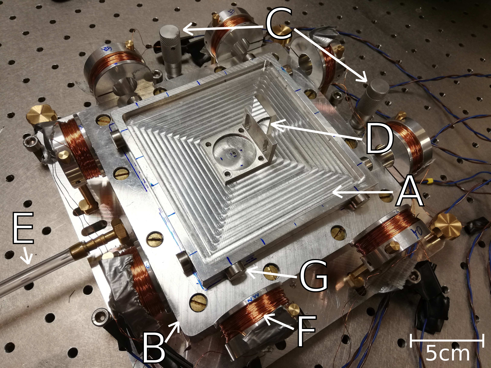
Figure 6
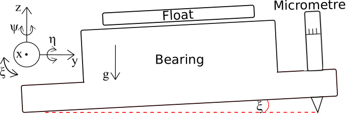
gives a schematic drawing of how the bearing can be tilted from the horizontal; where this can be done along the float’s x and y axes in the horizontal plane. Tilt in the y-axis by a known tilt angle, , is depicted in the figure.
IV Results
The torque acting on the float could be measured from the PID servo output, whose control loop is shown in Figure 7.

The PID servo applied a torque, , to the float by adding or subtracting from the bias currents in the appropriate coils. All eight coils were used for this purpose, and the bias currents are those described in Equations 14, 15 and 16. The magnitude of this change in current from the bias currents could then be used in conjunction with Equation 3 multiplied by the actuator arm length term, , from Table 1 to give
| (17) |
for eight coils. This measured torque is assumed to be equal to that described by Equation 15. The rotational stiffness could be measured by recording the change in torque, , from Equation 17 applied by the PID servo to the float after an offset equivalent to a known angle, , was added to the input of the controller. The rotational stiffness would then be given by
| (18) |
where this rotational stiffness is assumed to be equal to that described by Equation 10 once it had been summed over all the coils. The linear transverse stiffness of the float in the x and y-axis of the horizontal plane as described in Figure 2 could be calculated using Equation 4 summed over the bias currents of the four coils in each respective axis. As stated in Section II, the positioning of the magnets was chosen to give .
Before torque measurements could be made the float’s centre-of-mass displacement from its NCB, from Equation 15, had to be made zero. This was done by placing small masses on the float in precise positions such that when tilting it from the horizontal the PID servo torque did not change within the limit of the servo readout noise. Doing this, while keeping the bias currents in all the coils equal such that was zero in Equation 15, implied that was equal to zero.
The PID servo torque on the float was then measured over a range of tilt angles from the horizontal, for a given set of bias currents. This was done in both the x and y-axis of the float as shown in Figure 2. The measurements in these axes are shown in Figures 8
and 9
respectively.
The total mass of the float, with the additional small masses used for minimising , was 338.66 g. This, along with the value of of (42.0 0.5) mm from Table 1, implied the expected gradient of the plots from Equation 16 should be (0.139 0.003) Nm/rad. The gradients from Figures 8 and 9 are (0.137 0.006) Nm/rad and (0.138 0.006) Nm/rad respectively. With the bias currents used and Equation 14, the expected change of the centre-of-buoyancy of the float in both the x and y-axis was (7.00 0.17) mm. Using the gradients from Figures 8 and 9, in conjunction with Equations 14 and 16, the measured changes in the centre-of-buoyancy in the x and y-axis were calculated to be (6.90 0.32) mm and (6.95 0.32) mm respectively. This shows we had succeeding in tuning the float’s centre-of-buoyancy to an accuracy of 0.3 mm.
With the bias currents in all coils set to 0.075mA, and Equation 10 summed over all eight coils, the float’s rotational stiffness was calculated to be (-14.73 0.41) Nm/rad. Using Equation 18 it was measured to be (-15.11 2.05) Nm/rad. With these bias currents, the float’s transverse stiffness in each horizontal axis, using Equation 4 summed over the four coils in each axis, was calculated to be (1.11 0.16) N/m. This gave a natural oscillation frequency in each axis of (0.29 0.04) Hz. All the results are summarised in Table 2.
| Attribute | Result |
|---|---|
| Plot Gradients | |
| Float x-Axis | (0.137 0.006) Nm/rad |
| Float y-Axis | (0.138 0.006) Nm/rad |
| Equation 16 Prediction | (0.139 0.003) Nm/rad |
| Centre-of-Buoyancy Change | |
| Float x-Axis | (6.90 0.32) mm |
| Float y-Axis | (6.95 0.32) mm |
| Equation 14 Prediction | (7.00 0.17) mm |
| Float Rotational Stiffness | |
| Measurement | (-15.11 2.05) Nm/rad |
| Equation 10 Prediction | (-14.73 0.41) Nm/rad |
| Float Transverse Stiffness and Frequencies | |
| Equation 4 x and y-Axis Calculation | (1.11 0.16) N/m |
| Oscillation Frequency x and y-Axis | (0.29 0.04) Hz |
V Discussion
The measurements in Figures 8 and 9 change linearly with tilt angle as expected from Equation 16. The gradients of these plots were expected to be 0.139 Nm/rad and the measured gradients all lie within of this value and within their uncertainty ranges. The calculated and measured changes in the centre-of-buoyancy displacement of the float from Figures 8 and 9 were also within of each other and within each others uncertainty ranges. Thus all the results are in excellent agreement with the theory. Crucially this demonstrates that it is possible to tune in-situ the centre-of-buoyancy of a suspended object and hence also possible to decouple its rotational motion from ground tilt and horizontal accelerations.
The measured and calculated rotational stiffnesses of the float were within of each other and within their respective uncertainty bounds. The magnitude of these values is an order of magnitude lower than the rotational stiffness of a torsion balance used in a recent determination of Newton’s constant of gravitation, which had a stiffness of approximately 218 Nm/rad Quinn et al. 2014. Additional actuators could increase the float’s transverse stiffness from the calculated values to make the float more transversely stable, and also allow the adjustment of its rotational stiffness. Preliminary measurements with this setup show that this is possible Speake and Collins 2018. The natural oscillation frequencies of the float in the transverse plane were calculated. With the float being levitated through an air bearing, it can be assumed that it’s motion was highly damped. As such in this case there was no risk of the oscillations significantly affecting the float’s motion.
The design could be improved to allow greater precision in the placement and adjustment of the different components to give more accurate results. The noise from the electronics of the positional photodiode was measured to be Nm/, while the total noise of the air bearing system was measured to be Nm/. This was the largest contribution to the data point uncertainties in Figures 8 and 9. This gave an error on the gradients of these plots, which was then propagated onto the experimental estimation of from Equation 14. No attempt was made to put the device in a protective enclosure or shield the photodiode from environmental light sources. As such the error on of 0.3 mm could be reduced by lowering the noise of the air bearing. This could be done by using a different method of levitation other than a pressurised-air suspension, such as an electrostatic or superconducting suspension Speake and Collins 2018. From Equation 14, the theoretical maximum accuracy of centre-of-buoyancy tuning that could be attained with the setup presented here, taking into account the current noise from the coil drivers of the magnetic actuators averaged over a second, is m. This corresponds to a possible improvement in accuracy of a factor of over 18000.
VI Conclusion
An air bearing suspension that levitates a float, with its motion in the horizontal plane of the laboratory controlled using magnetic actuators, was constructed. The observed behaviour of the float was compared to the predictions of a detailed model of the statics of the float-actuator system and they were found to be consistent. The results from Figures 8 and 9 demonstrate the in-situ electromagnetic tuning of the float’s centre-of-buoyancy to an accuracy of 0.3 mm. This result implies it is practical to decouple the rotational mode of a suspended object from tilt and horizontal accelerations due to seismic noise, by tuning its centre-of-buoyancy to lie at its nominal centre-of-buoyancy (NCB).
This result paves the way for other, more sensitive, experiments to be designed with a view to performing weak-force measurements at sub-mm ranges. Work is ongoing on a superconducting torsion balance Speake and Collins 2018; Chalkley et al. 2011. The aim here is to develop an instrument which exhibits the same advantages as the air bearing where it can be tuned in-situ to be rotationally decoupled from ground tilt, in addition to allowing the in-situ tuning of its rotational stiffness. This combined with a transverse stiffness provided by the superconducting magnetic actuators should allow measurements of the inverse square law of gravity down to mass separations of the order of 10m. The Newtonian torque signal, given a day’s integration, requires a fundamental noise level of less than Nm/. Given a typical seismic noise acceleration spectral density of m/s and a suspended mass of 338.66 g, we would need to match the centre-of-buoyancy and mass to an accuracy of about m. So an improvement in tuning accuracy of a factor of around a thousand would be required compared with what is achieved here. The uncertainty on the matching of the centres-of-mass and buoyancy is limited by the overall noise in the air bearing system, so this goal may be achievable with a superconducting or other type of suspension. We should also mention that a possible downside of this technique is the way that the actuation system can introduce noise into the measurement through its asymmetries (the parameter introduced in Equation 15). Any strategy of reducing this factor would include making such asymmetries as small as possible in the first instance, thus ensuring that the actuation torques themselves are as small as possible.
Acknowledgements.
We would like to thank Dr. Chris Collins for helpful discussions. We would also like to thank Masters project students Joseph Parker, Jack Joynson, Hugo Yamaguchi and Arthur O’Leary for their help in this project. We would additionally like to thank John Bryant and David Hoyland in helping to design and build the PID servo system in LabVIEW and the ADC/DAC setup for the experiment. We are grateful to UK STFC (Grant No. ST/F00673X/1) who initially supported this work. We are also very grateful to Leverhulme (Grant No. RPG-2012-674) for financial support.References
- Cavendish (1798) H. Cavendish, Philosophical Transaction of the Royal Society of London 88(5-6), 469 (1798).
- Newman, Berg, and Boynton (2009) R. D. Newman, E. C. Berg, and P. E. Boynton, Space Science Reviews 148, 175 (2009).
- Murata and Tanaka (2015) J. Murata and S. Tanaka, Classical and Quantum Gravity 32 (2015), 10.1088/0264-9381/32/3/033001.
- Lamoreaux (2005) S. K. Lamoreaux, Reports on Progress in Physics 68, 201 (2005).
- Wagner et al. (2012) T. A. Wagner, S. Schlamminger, J. H. Gundlach, and E. G. Adelberger, Classical and Quantum Gravity 29 (2012), 10.1088/0264-9381/29/18/184002.
- Gillies and Ritter (1993) G. T. Gillies and R. C. Ritter, Review of Scientific Instruments 64, 283 (1993).
- Adelberger et al. (2009) E. G. Adelberger, J. H. Gundlach, B. R. Heckel, S. Hoedl, and S. Schlamminger, in Progress in Particle and Nuclear Physics, Vol 62, No 1, Progress in Particle and Nuclear Physics, Vol. 62, edited by A. Faesssler (Elsevier Science B.V., Sara Burgerhartstrat 25, PO Box 211, 1000 AE Amsterdam, Netherlands, 2009) pp. 102–134.
- McManus et al. (2017) D. J. McManus, P. W. F. Forsyth, M. J. Yap, R. L. Ward, D. A. Shaddock, D. E. McClelland, and B. J. J. Slagmolen, Classical and Quantum Gravity 34, 135002 (2017).
- Shimoda and Ando (2019) T. Shimoda and M. Ando, Classical and Quantum Gravity 36, 125001 (2019).
- Mow-Lowry and Martynov (2019) C. M. Mow-Lowry and D. Martynov, Classical and Quantum Gravity 36, 245006 (2019).
- Speake and Newell (1990) C. C. Speake and D. B. Newell, Review of Scientific Instruments 61, 1500 (1990).
- Harms and Venkateswara (2016) J. Harms and K. Venkateswara, Classical and Quantum Gravity 33 (2016), 10.1088/0264-9381/33/23/234001.
- Speake and Collins (2018) C. C. Speake and C. J. Collins, Physics Letters A 382, 1069 (2018).
- Joynson (2019) J. Joynson, Air-Bearing Suspension with Passive Magnetic Stabilisation and Tuning, Master’s thesis, University of Birmingham (2019).
- Quinn et al. (2014) T. Quinn, C. C. Speake, H. Parks, and R. Davis, Philosophical Transactions of the Royal Society A-Mathematical Physical and Engineering Sciences 372 (2014), 10.1098/rsta.2014.0032.
- Smythe (1989) W. R. Smythe, Static and Dynamic Electricity, 3rd ed. (Taylor & Francis, 1989).
- Aston and Hoyland (2004) A. Aston and D. Hoyland, “Osem interface control document,” Advanced LIGO UK Internal Document LIGO-T050111-06-K (University of Birmingham, 2004).
- Chalkley et al. (2011) E. C. Chalkley, S. Aston, C. C. Collins, M. Nelson, and C. C. Speake, in The XLVIth Rencontres de Moriond and GPhyS Colloqium 2011 (2011) pp. 207–210.
*