Collisionless particle dynamic in an axi-symmetric diamagnetic trap
Abstract
Particle dynamic in an axi-symmetric mirror machine with an extremely high plasma pressure equal to pressure of vacuum magnetic field (so-called regime of diamagnetic confinement) is investigated. Extrusion of magnetic field from central region due to plasma diamagnetism leads to non-conservation of the magnetic moment and can result in chaotic movement and fast losses of particles. The following mechanisms can provide particle confinement for unlimited time: absolute confinement of particles with high azimuthal velocity and conservation of adiabatic invariant for particle moving in smooth magnetic field. The criteria of particle confinement and estimations of lifetime of unconfined particles are obtained and verified in direct numerical simulation. Particle confinement time in the diamagnetic trap in regime of gas-dynamic outflow is discussed.
November 2019
Keywords: mirror machine, high-beta plasma, diamagnetic confinement, particle dynamic in magnetic field
1 Introduction
Newly proposed regime of diamagnetic confinement of plasma in a mirror machine [1] allows us to essentially reduce particles and energy losses from the trap and increase power density of thermonuclear reactions. The idea is to confine plasma with extremely high pressure equal to pressure of magnetic field of the trap. It leads to formation of central region with sharp boundary occupied by dense plasma with extruded magnetic field (so called diamagnetic “bubble”). The effective mirror ratio inside the “bubble” is extremely high, so in MHD approximation longitudinal losses of plasma from inner area of the diamagnetic trap are suppressed. In frame of the MHD approximation the plasma and energy losses are driven by diffusion of plasma through magnetic field on the border of the “bubble” [1, 2]. There losses grow linearly with increasing “bubble” length and radius and are reduced when plasma conductivity rises.
The structure of magnetic field in the diamagnetic trap is close to Field Reversal Configuration (FRC) [4] with zero field reversal. So particle dynamic in the diamagnetic trap has a lot in common with dynamic of fast ions in FRCs.
Investigation of single-particle dynamic in the diamagnetic trap is needed for development of kinetic models of diamagnetic confinement. Small magnitude of magnetic field results in non-conservation of magnetic moment and can lead to chaotic behavior and fast longitudinal losses of particles. From the other hand, particle energy and canonical angular momentum are integrals of motion due to stationarity and azimuthal symmetry of magnetic field. The aim of this work is investigation of regimes of particle confinement and lifetime of unconfined particles in the diamagnetic trap.
The magnetic field is assumed to be fully axisymmetric later. So influence of possible instabilities and non-accuracy of magnetic system of the trap are neglected. Non-symmetry of magnetic system is seems to result in slow Arnold diffusion of energy and angular moment. In presence of dense plasma the Coulomb collisions should to masque the slow diffusion. Mechanisms of anomalous losses due to plasma instabilities in diamagnetic trap are addressed for future investigations.
The article is organized as follow. Hamilton function of particle in the trap is discussed in the second section. Two mechanisms can provide particle confinement in unlimited time if collision scattering is absent, namely so-called absolute confinement [3] and conservation of radial adiabatic invariant. There mechanisms are discussed in the third section. The estimations for lifetime of unconfined particles and plasma confinement time in gas-dynamic regume are found in the fourth and fifth sections. Simple numerical example is presented in the sixth section. The results are discussed in the Conclusion.
2 Hamiltonian
We consider particle dynamic in the axisymmertic magnetic field without spirality. This field can be described by only one function, namely magnetic flux , here , and are azimuthal component of vector potential, radial and longitudinal coordinate. The Hamilton function can be written in the following form
| (1) |
here is electrostatic ambipolar potential. The particle energy and canonical angular momentum are integrals of motion due to stationarity and azimuthal symmetry. If structure of magnetic field is “bubble”-like that magnetic field (and magnetic flux) is small inside region in central part of the trap. Outside this region magnetic field is approximately vacuum (examples of structure of magnetic field are shown in [1, 2], see also figures 2 and 3). We assume that the ambipolar potential is approximately constant in region with very small magnetic field and that longitudinal gradient scale of the potential on “bubble” boundary coincides with longitudinal gradient scale of magnetic field.
It is convenient in numerical simulations to express all dimension quantities via particle mass, vacuum magnetic field in the center of the trap and cyclotron frequency calculated by vacuum magnetic field . Only quantities with dimension of length remain after this expressing. So integrals of motion with dimension of length will be used later together with energy and angular momentum, namely Larmor radius calculated by full energy and vacuum magnetic field and minimal possible distance between particle and axis in case of zero magnetic field .
An example of trajectories in the transversal cross-section are shown in figure 1. Radial dependence of the magnetic field is chosen in the form , here . The trajectories can be divided into three classes in dependence on sign of particle angular momentum. Orbits of the particles with and correspond to betatron and drift orbits in FRC [6]. As in the FRC, confinement of particles essentially depends on sign and magnitude of angular momentum (see below).


3 Regimes of particle confinement
Non-conservation of magnetic momentum due to smallness of magnitude of magnetic field inside the diamagnetic “bubble” results in changing of regimes of particle confinement and essentially modification of concept of loss cone. Two mechanisms can provide particle confinement in the diamagnetic trap for unlimited time (in absence of collision scattering and non-axisymmetry): well-known absolute confinement [3] and conservation of radial adiabatic invariant.
3.1 Absolute confinement
The mechanism of the absolute confinement is follow. The Hamiltonian (1) described two-dimensional motion in effective potential . This potential is potential well for particles with . Such particles confines in the trap if their energy is small enough.
To find condition of the absolute confinement one can note that in region of mirrors the magnetic field if quasi-uniform, , here is vacuum mirror ratio of the trap. Let’s found minimal possible energy of particle moving with angular momentum in the mirror region. Minimal value of effective potential is reached at a point with radial coordinate which satisfies equation , here is radial distribution of ambipolar potential in mirror. Minimal energy is . Particle with angular momentum cannot penetrate in region of the mirror if their energy less than .
In simplest case of zero electrostatic potential and criterion of absolute confinement can be written in the form [3]
| (2) |
This criterion can be re-written in another form: and . Particle is confined absolutely if it rotates quickly in the direction which coincides with direction of cyclotron rotation.
Preferential confinement of ions with negative angular momentum can results in spontaneous rotation of plasma in the trap which is similar to particle-loss spin-up in FRCs [4].
3.2 Adiabatic confinement
Radial adiabatic invariant
| (3) |
conserves if magnetic field changes in longitudinal direction smoothly and particle longitudinal velocity is not too large. In this case frequency of radial oscillations
| (4) |
can be much greater than inverse time of varying of magnetic field during particle longitudinal motion. It should be noted that regular motion of ions in oblate FRCs due to conservation of adiabatic invariant is observed also in numerical simulations of FRCs (see, for example, [5]).
If vacuum magnetic field has one local minimum (corrugation of field is absent) than character time of varying of magnetic field during particle longitudinal motion is ratio of distance between mirrors to longitudinal velocity so criterion of adiabaticity is . Let us consider case of large radius of diamagnetic “bubble” . In this case it is convenient to introduce radial coordinate of magnetic field line on the “bubble” boundary . To choose this field line the condition is used. If and electrostatic potential is zero one can calculate (here ) and write criterion of adiabaticity in the form
| (5) |
Expression denotes maximal value of derivative of function . We assume that radial distribution of ambipolar potential is approximately constant inside the “bubble” and that longitudinal gradient scale of ambipolar potential is of the order of . In this case taking the electrostatic potential into account does not changes criterion (5) essentially.
If motion of particle is regular than particle is confined in the trap if real solutions of equation are absent (here are coordinates of mirrors). Magnetic flux in the mirror is approximately equal to flux of vacuum magnetic field . So adiabatic invariant (3) in the mirror is equal to , here is Heaviside step function and is radial distribution of ambipolar potential in mirror (we assume that Larmor radius of particle in mirror is small in comparison with radial scale length for potential). Criterion of confinement of regularly moving particle can be written in the form
| (6) |
Criterion (6) can be written in analytical form if radius of the “bubble” is large, , and ambipolar potential is approximately constant inside the “bubble”. In this case the invariant (3) is equal approximately to the radial adiabatic invariant for particle moving inside long cylinder surface with radius :
3.3 Criterion of adiabaticity in corrugated field
Discrete structure of magnetic system leads to corrugation of vacuum magnetic field which results in corrugation of margin of diamagnetic bubble. So time of essential changing of magnetic field during longitudinal motion essentially decreases and can become comparable with period of radial oscillations (such effect for particles moving in vacuum magnetic field is described in [8]). Resonant interaction between radial oscillations and longitudinal motion can destroy adiabatic invariant (3) even if criterion of adiabaticity (5) is satisfied. In this section we will estimate magnitude of corrugation of vacuum magnetic field at which corrugation not influence on movement of particle.
Let’s look a longitudinally-uniform diamagnetic trap with weak corrugation of vacuum magnetic field. Flux of vacuum magnetic field is , vacuum magnetic field at is . Flux of field in the trap is the sum , unperturbed part satisfies integral equation [6]
| (7) |
here is azimuthal component of plasma current (which depends on distribution function of ions and electrons),
is Green function (magnetic flux generated by electric current flowing on a cylindrical surface with radius ), is radius of conducting shell surrounding plasma, is Heaviside step function.
Perturbed part satisfies following linear integral equation:
with the Green function (which is solution of the equation )
The hamiltonian of particle moving in longitudinally-uniform diamagnetic trap with weak corrugation is
One can make canonical transformation to the action-angle variables of non-perturbed hamiltonian:
here is radial adiabatic invariant, , is radial velocity, is solution of equation . Radial coordinate depends periodically on new variable (because depends periodically on time) so perturbation of hamiltonian can be expanded in a Fourier series:
| (8) |
Condition of resonance between radial oscillations and longitudinal motion is .
Concrete form of the distribution functions of ions and electrons are needed to calculate magnetic flux and coefficients in (8) and to follow investigation of adiabacity. Analytical treatment can be extended in the following cases: if angular momentum of particle is negative and small enough and if radius of the diamagnetic bubble exceeds essentially particle Larmor radius .
3.3.1 Particles with .
Now we consider particles with negative and very small angular momentum. Ions with such momentum can arises in the trap due to off-axis NBI. This ions move along betatron orbits with small harmonic oscillations in radial direction. The unperturbed part of hamiltonian can be written as [9]
here is solution of equation (mean radius of betatron orbit), is betatron frequency, is local cyclotron frequency. Amplitude of betatron oscillations is assumed to be small, .
Transition to the angle-momentum variables describes by canonical transformation
After transition to the angle-momentum variables the Hamiltonian transforms to
| (9) |
Resonances between radial oscillations and longitudinal motion are absent in the hamiltonian (9) so the particles move adiabatically. Condition of applicability of this approximation can be written in the form
This condition means that frequency of radial oscillations (which is the betatron frequency) have to be large enough.
3.3.2 Particles with .
If radius of the diamagnetic “bubble” is much greater than width of transition layer and “Larmor radius” that motion of particles can be described approximately as motion of particle inside surface rotation . Here function is coordinate of magnetic field line at boundary of the bubble.
Let’s found the criterion of adiabaticity of particle moving with velocity inside corrugated cylinder when corrugation is small, and . Particle dynamic is described by twist mapping (see Appendix A)
| (10) |
here and are longitudinal velocity and coordinate at times when radial component of velocity is zero, is the ratio of longitudinal and transversal components of velocity, is amplitude of radial oscillations and .
After linearization near resonances (here are solutions of equation with integer ) and transition to new variable one can write the twist mapping (10) in the form of the Chirikov standard map
here is so-called stochasticity parameter. To estimate magnitude of corrugation needed for destroying adiabatic invariant we use the Chirikov criterion of resonances overlapping
| (11) |
and estimation of magnitude of corrugation of boundary of diamagnetic “bubble” found in MHD approximation [2]
| (12) |
For small-scale perturbations with estimation (12) can be simplified:
| (13) |
We combine expressions (11) and (13) to found criterion of adiabaticity of motion in the diamagnetic trap for particles with :
| (14) |
here .
This condition is first broken for particles with zero angular momentum, . Most dangerous are small-scale perturbations with , but magnitude of perturbations with very large is seems to be small due to finite Larmor radius effects which is neglected in expression (12). Particles with great value of move adiabatically which consistent with results of previous section. Particles with great value of move in region outside the bubble where magnetic field is strong so this particles moves adiabatically also. This behavior consistents with criterion (14).
4 Lifetime of unconfined particles
Let’s us now looks particles which move chaotically and are not confined absolutely. If particle moves regularly than particle arrival to mirror at the same longitudinal velocity after each excursion from mirror to mirror. If radial adiabatic invariant not conserves than longitudinal velocity changes chaotically with each approach to mirror so particle leave the diamagnetic trap after several excursions from mirror to mirror. To estimate lifetime of chaotically moving particles we consider population of particles with same energy and angular momentum which move inside quasi-cylindrical diamagnetic “bubble” with radius and length . Distribution function of this particles is , here is solution of equation , is value of longitudinal velocity corresponding margin of adiabaticity. Full number of particles in the trap and particle flow through mirrors are approximately
here is coordinate of the mirror. Particle lifetime is .
In the simplest case when all particles with energy and angular momentum move chaotically, , “bubble” radius is large, , and electrostatic potential is neglectingly small, estimation of particle confinement time is:
here is of the order of particle transit time from mirror to mirror (period of bounce-oscillations).
5 Estimation of plasma lifetime in gas-dynamic regime
Calculation of particle confinement time in regime of diamagnetic confinement requires sophisticated calculations including solving of kinetic equation together with equilibrium equation. This calculation can be essentially simplified if plasma is quite dense and angular scattering time is less than lifetime of unconfined particles. In this case particle distribution functions are locally Maxwellian and one can estimate particle confinement time by calculating full number of particles and their flow through mirrors.
Let’s assume that distribution function of particles of type approximately coincides with distribution of Maxwellian particles inside cylinder with radius
| (18) |
This distribution allows particle density to be uniform inside the diamagnetic “bubble” with radius , like in MHD models (see next section). One can estimate lifetime of particles with distribution as
| (19) |
here is thermal velocity of particles of type , is mean Larmor radius calculated by vacuum magnetic field. Estimation (19) gives same lifetime for ions and electrons with same temperatures so plasma outflow in such regime should not be accompanied by appearing essential ambipolar potential.
Combination is of the order of time of gas-dynamic outflow from trap with vacuum magnetic field . So transition to regime of diamagnetic confinement increases times particle confinement time in gas-dynamic regime. This estimation should be compared with estimation
of particle confinement time in MHD model [1, 2], here is thickness of boundary layer in MHD approximation. This comparison demonstrates that kinetic effects are important when .
It should be noted that effects of adiabatic confinement of part of particles not taken into account in estimation (19). This effects can be important if plasma flow through mirror is collisionless (“short” mirrors). Effects of adiabatitity of motion are seems to decrease particle losses. In this sense the estimation (19) is most pessimistic estimation of particle confinement time in the gas-dynamic regime.
6 Numerical example
To illustrate influence of structure of magnetic system on collision-less particle dynamic some results of numerical simulation of ions movement in diamagnetic trap are presented in this section. Magnetic flux is calculated similarly article [6]. Namely, magnetic flux satisfies Amperes’s law (here is azimuthal component of plasma current) which can be write in the form of integral equation
| (20) |
here is flux of vacuum magnetic field and
is Green function (magnetic flux of thin coil), and are complete elliptic integrals of first and second kinds, .
The integral equation (20) can be solved numerically by iterations. To calculate plasma current we assume electrons to be cold and choose distribution function of ions (18). Dependence of density and azimuthal current of ions on radial coordinate and magnetic flux are given in Appendix B. Example of radial dependence of plasma density and longitudinal component of magnetic field on radius is shown on figure 2. Plasma density is constant inside the “bubble” like in the MHD model [1, 2].

Magnetic system of trap consists of two mirror coils and of set of equidistant coaxial coils which generate quasi-uniform magnetic field (see figure 3). In one case corrugation of vacuum magnetic field does not exceeds tenths of percent (smooth magnetic field). In second case distance between the coils is doubled and radius of the coils is reduced (currents in coils are changed correspondingly so that value of magnetic field in center is the same in both cases). It results in observable corrugation of the “bubble” boundary.


Numerical simulation allows us to found maximal value of longitudinal velocity at which ions confine in the trap. Ions move regularly in trap with smooth field and maximal critical velocity is restricted only by criterion of confinement (6). An example of dependence of critical velocity on angular momentum for ions moving in trap with corrugated field is shown on figure 4. Ions with small scatter due to corrugation so their critical velocity is relatively low. This velocity increases when rises (in according with criterion of adiabaticity (14)). Ions with negative and small are confined absolutely so their maximal velocity is restricted by full energy . Critical velocity of ions with large decreases because this ions move in region with finite magnetic field outside the “bubble”.

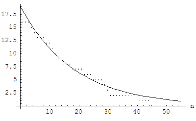
An example of number of unconfined ions in trap with corrugated field after bounce-oscillations is shown on figure 5. This number decreases approximately exponentially with time. Confinement time is consistent with analytical estimation (4).
7 Conclusion
Smallness of magnetic field in central region of the diamagnetic trap results in non-conservation of magnetic moment so regimes of particle confinement are modified. Particle can confine inside the diamagnetic “bubble” either due to conservation of radial adiabatic invariant (this mechanism occurs if vacuum magnetic field is smooth) or in regime of adiabatic confinement (if particle rotates quickly around axis of trap in direction coinciding with direction of cyclotron rotation). Possibility of conservation of the adiabatic invariant depends strongly on geometry of magnetic field, especially on small-scale perturbation of vacuum magnetic field. Lifetime of unconfined particles increases with increasing the “bubble” radius and vacuum magnetic field in the mirrors of the trap and decreasing particle “Larmor radius” . Even in the worst case when all particles move chaotically particle confinement time exceeds the gas-dynamic time in the vacuum field in ratio of the “bubble” radius to mean ion “Larmor radius”.
The author wish to thank all the members of the laboratories 9-0, 9-1 and 10 of BINP SB RAS who participated in discussion of the results of this work. Author especially grateful to the Dr. Alexei Beklemishev, Dr. Dmitriy Skovorodin and Mikhail Khristo for fruitful discussions.
8 Appendix A. Twist mapping for particle inside corrugated surface
Now we consider particle moving with velocity inside corrugated cylindrical surface and reflecting elastically from it. Let and to be longitudinal coordinate and longitudinal component of velocity of particle at time . At this point of time radial velocity equal to zero and azimuthal component of velocity is . Radial coordinate of particle is , here . Particle will collide with surface at point of time which is solution of equation . Longitudinal and radial coordinate of the particle at the moment of collision are and . Radial, azimuthal and longitudinal components of velocity at the moment of collision are , è . After collision radial and longitudinal components of velocity are è , here . Azimuthal component does not change. Radial coordinate of particle will reach minimal value through time after collision. Longitudinal velocity is when radial coordinate is minimal.
If corrugation is weak that time before collision is approximately , here and . When radial coordinate minimal longitudinal component of velocity and longitudinal coordinate of particle are described by expressions (10).
9 Appendix B. Density and current of ions.
Density of ions with distribution function (18) is
here is normalized magnetic flux, is electrostatic potential, is thermal velocity and
Current of ions is
References
- [1] A.D. Beklemishev. Diamagnetic “bubble” equilibria in linear traps // Physics of Plasmas 23, 082506 (2016), doi: 10.1063/1.4960129
- [2] A.D. Beklemishev and M.S. Khristo. High-Pressure Limit of Equilibrium in Axisymmetric Open Traps // Plasma and Fusion Research 14 2403007, (2019), doi: 10.1585/pfr.14.2403007
- [3] Ming-Yuan Hsiao and George H. Miley. Velocity-space particle loss in field-reversed configurations // Physics of Fluids 28, 5, (1985), doi: 10.1063/1.864978
- [4] Loren C. Steinhauer. Review of field-reversed configurations // Physics of Plasmas 18 070501 (2011), doi: 10.1063/1.3613680
- [5] Elena V. Belova, Ronald C. Davidson, Hantao Ji, and Masaaki Yamada. Advances in the numerical modeling of field-reversed configurations // Physics of Plasmas 13 056115 (2006); doi: 10.1063/1.2179426
- [6] Artan Querushi and Norman Rostoker. Equilibrium of field reversed configurations with rotation. I. One space dimensions and one type of ion // Physics of Plasmas 9 3057 (2002), doi: 10.1063/1.1475683
- [7] Artan Querushi and Norman Rostoker. Equilibrium of field reversed configurations with rotation. IV. Two space dimensions and many ion species // Physics of Plasmas 10 737 (2003), doi: 10.1063/1.1539853
- [8] B.V. Chirikov. Resonance processes in magnetic traps // J. Nucl. Energy, Part C Plasma Phys 1 253 (1960).
- [9] H. Vernon Wong, H. L. Berk, R. V. Lovelace, and N. Rostoker. Stability of annular equilibrium of energetic large orbit ion beam // Physics of Fluids B: Plasma Physics 3 2973 (1991), doi: 10.1063/1.859931