Graph Neural Distance Metric Learning with Graph-Bert
Abstract
Graph distance metric learning serves as the foundation for many graph learning problems, e.g., graph clustering, graph classification and graph matching. Existing research works on graph distance metric (or graph kernels) learning fail to maintain the basic properties of such metrics, e.g., non-negative, identity of indiscernibles, symmetry and triangle inequality, respectively. In this paper, we will introduce a new graph neural network based distance metric learning approaches, namely GB-Distance (Graph-Bert based Neural Distance). Solely based on the attention mechanism, GB-Distance can learn graph instance representations effectively based on a pre-trained Graph-Bert model. Different from the existing supervised/unsupervised metrics, GB-Distance can be learned effectively in a semi-supervised manner. In addition, GB-Distance can also maintain the distance metric basic properties mentioned above. Extensive experiments have been done on several benchmark graph datasets, and the results demonstrate that GB-Distance can out-perform the existing baseline methods, especially the recent graph neural network model based graph metrics, with a significant gap in computing the graph distance.
Keywords:
Machine Learning, ICML1 Introduction
Graph provides a general representation of many network structured data instances in the real world, which can capture both the properties of nodes and the extensive connections among the nodes. For instance, the app function-call diagrams (Hu et al. 2009), brain-region functional activities (Bullmore & Bassett 2011) and the bio-medical drug molecules (Duvenaud et al. 2015) can all be represented as graphs in various shapes. An important research problem in graph studies is to learn the distance metric of the graph instances (Bunke 1997; Gao et al. 2010; Bunke & Shearer 1998), which can serve as the foundation of many other research tasks, e.g., molecular graph clustering (Jin et al. 2018), brain graph classification (Richiardi et al. 2013) and frequent sub-graph extraction (Yan & Han 2002). In this paper, we will not distinguish the differences among graph distance, graph similarity and graph kernel learning problems, and unify them all as the graph distance metric learning problem.
Graph instance distance metric learning is an interesting research problem, and many research works have been done on this topic. In early years, to measure the distance between graphs, graph edit distance (Bunke 1997; Gao et al. 2010) and maximum common subgraph (Bunke & Shearer 1998) are commonly used. The distance metrics defined by these two methods can convey concrete physical meanings (i.e., edit distances and subgraph), but these methods are also known to be NP-complete (Bunke & Shearer 1998; Zeng et al. 2009). In the past few years, we have witnessed new developments on graph distance metric learning, many of them are based on the graph neural network models (Li et al. 2019; Bai et al. 2019). In (Li et al. 2019), a new model named graph matching network is introduced, which adopts the propagation layer in the model for learning the node distance scores between graphs. Meanwhile, in (Bai et al. 2019), the authors propose to apply the latest graph convolutional network for node representation learning prior to computing the graph distance scores.
However, via a thorough analysis about the existing graph distance metrics, several common disadvantages about them can be identified, which are listed as follows:
- •
High Computational Cost: For the traditional graph edit distance or subgraph learning based methods, the metric score computational process can be extremely time-consuming. Meanwhile, for the pair-wise graph neural distance metrics, the model training cost will grow quadratically as the graph number increases.
- •
Node-Order Invariant Representation: For the latest graph neural network based methods, which take neural network models as the representation learning component, the learned graph instance representations and the distance metric scores will vary greatly as the input graph node order changes.
- •
Semi-Supervised Learning: To train the neural network based methods, a large number of graph-pair distance scores need to be labeled in advance, which can be very tedious and time consuming. The existing works mostly fail to utilize the unlabeled graph pairs in the metric learning.
- •
Lack of Metric Properties: Furthermore, for most of the existing graph distance metric learning approaches, they fail to maintain the basic properties of the metrics (Sra et al. 2005; Wikipedia 2019) in the learning process, like non-negativity, identity of indiscernibles, symmetry and triangle inequality, respectively.
In this paper, we aim to introduce a new graph distance metric learning approach, namely GB-Distance (Graph-Bert based Neural Distance), to resolve the disadvantages with the existing works mentioned above. GB-Distance is based on the state-of-the-art Graph-Bert model (Zhang et al. 2020), which is capable to learn effective graph representations based on the attention mechanism.
Meanwhile, for efficient and effective metric scores computation, GB-Distance further modifies Graph-Bert in several major perspectives by (1) extending Graph-Bert for graph instance representation learning (Graph-Bert is proposed for graph node embedding originally), (2) introducing pre-training and fine-tuning to graph neural distance metric learning to lower down the learning costs, and (3) proposing new node-order invariant initial input embeddings and model functional components. What’s more, GB-Distance works very well in the semi-supervised learning setting and can also effectively incorporate various metric properties in the learning process as additional constraints of the objective function.
The remaining sections of this paper are organized as follows. We will first talk about the related works in Section 2, and then introduce the notations, terminology definitions and problem formulation in Section 3. Detailed information of the GB-Distance model is provided in Section 4, whose effectiveness will be tested with experiments on real-world benchmark datasets in Section 5. At the end, we will conclude this paper in Section 6.
2 Related Work
In this section, we will briefly introduce the related work on graph neural network, graph metric learning, metric optimization and BERT.
Graph Neural Network: In addition to the graph convolutional neural network (Kipf & Welling 2016) and its derived variants (Veličković et al. 2018; Li et al. 2018; Sun et al. 2019; Lin et al. 2019), many great research works on graph neural networks have been witnessed in recent years. In (Meng & Zhang 2019), the authors introduce the graph isomorphic neural network, which can automatically learn the subgraph patterns based representations for graphs. In (Zhang et al. 2020), the authors introduce a new type of graph neural network based on graph transformer and BERT. Many existing graph neural network models will suffer from performance problems with deep architectures. In (Zhang & Meng 2019; Li et al. 2018; Sun et al. 2019; Huang & Carley 2019), the authors explore to build deep graph neural networks with residual learning, dilated convolutions, and recurrent network, respectively. A comprehensive survey of existing graph neural networks is also provided in (Zhang 2019; Wu et al. 2019).
Graph Metric Learning: In addition to the classic graph edit distance (Bunke 1997; Gao et al. 2010) and common subgraph (Bunke & Shearer 1998) based graph distance metrics, there also exist several important recent research works on graph distance metric learning (Kondor & Pan 2016; Togninalli et al. 2019; Yanardag & Vishwanathan 2015; Li et al. 2019; Bai et al. 2019; Shervashidze et al. 2009). (Shervashidze et al. 2009) proposes to compare graphs by counting graphlets; (Yanardag & Vishwanathan 2015) learns latent representations of sub-structures for graphs with deep neural networks; (Togninalli et al. 2019) defines the graph kernels based on the Wasserstein distance between node feature vector distributions of two graphs; and (Kondor & Pan 2016) introduces a multi-scale Laplacian graph kernel instead. (Li et al. 2019) adopts the propagation layer in the model for learning the node distance scores between graphs, and (Bai et al. 2019) utilizes the graph convolutional network for representation learning prior to computing graph distance. However, these existing graph metric learning methods suffer from either the lack of interpretability or the high computational costs.
Metric Optimization: Distance metric learning is a classic research task in machine learning, a comprehensive survey on which is also available at (Yang & Jin 2006). In (Xing et al. 2003), the authors formulate the distance metric learning as a convex optimization problem, which also proposes an efficient and local-optima-free learning algorithm to solve the problem. In (Ying & Li 2012), the distance metric learning is defined as an eigenvalue optimization problem instead. In (Sra et al. 2005), the authors further consider the basic properties on distance metrics, which formulate the problem as a constrained optimization problem. They also introduce an efficient learning algorithm to maintain the triangle inequality subject to the norm.
BERT and Transformer: In NLP, the dominant sequence transduction models are based on complex recurrent (Hochreiter & Schmidhuber 1997; Chung et al. 2014) or convolutional neural networks (Kim 2014). However, the inherently sequential nature precludes parallelization within training examples. Therefore, in (Vaswani et al. 2017), the authors propose a new network architecture, i.e., the Transformer, based solely on attention mechanisms, dispensing with recurrence and convolutions entirely. With Transformer, (Devlin et al. 2018) further introduces Bert for deep language understanding, which obtains new state-of-the-art results on majority of the natural language processing tasks.
3 Notations and Problem Formulation
In this section, we will introduce the notations used in this paper, and provide the formulation of the studied problem.
3.1 Notations
In the sequel of this paper, we will use the lower case letters (e.g., ) to represent scalars, lower case bold letters (e.g., ) to denote column vectors, bold-face upper case letters (e.g., ) to denote matrices, and upper case calligraphic letters (e.g., ) to denote sets or high-order tensors. Given a matrix , we denote and as its row and column, respectively. The (, ) entry of matrix can be denoted as either or , which will be used interchangeably. We use and to represent the transpose of matrix and vector . For vector , we represent its -norm as . The Frobenius-norm of matrix is represented as . The element-wise product of vectors and of the same dimension is represented as , whose concatenation is represented as .
3.2 Problem Formulation
The data instances studied in this paper are all in the graph structure, which can be denoted as the graph instance.
Definition 1
(Graph Instance): Formally, a graph instance can be represented as , where and denote the sets of nodes and links, respectively. Mapping projects the nodes to their corresponding raw attributes in space . For presentation simplicity, we can also denote the raw feature vector of as . Meanwhile, the mapping can project node pairs to their corresponding link weights. For any non-existing link , we have by default.
The above definition provides a general representation for graph instances. For the graph raw attributes, they can denote various types of information actually depending on the application settings, e.g., images, textual descriptions and simple tags. Meanwhile, if the graph instances studied are unweighted, we will have , and . Based on the above definition, we can define the problem studied in this paper as follows.
Problem Statement: Formally, given a set of graph instances (the superscript denotes the graph index), in this paper, we aim to learn a mapping to compute the distance for any graph instance pairs from . Here, mapping should also maintain the basic distance metric properties, i.e., non-negativity, identity of indiscernibles, symmetry and triangle inequality. Detailed representation of these different properties will be illustrated in the following section.
4 Method
In this section, we will introduce the GB-Distance model. At the beginning, we will provide the description of the architecture of GB-Distance first, whose internal functional components will be introduced in detail in the follow-up subsections. At the end, we will talk about the mathematical constraints for modeling the metric properties in the learning process.
4.1 Framework Description
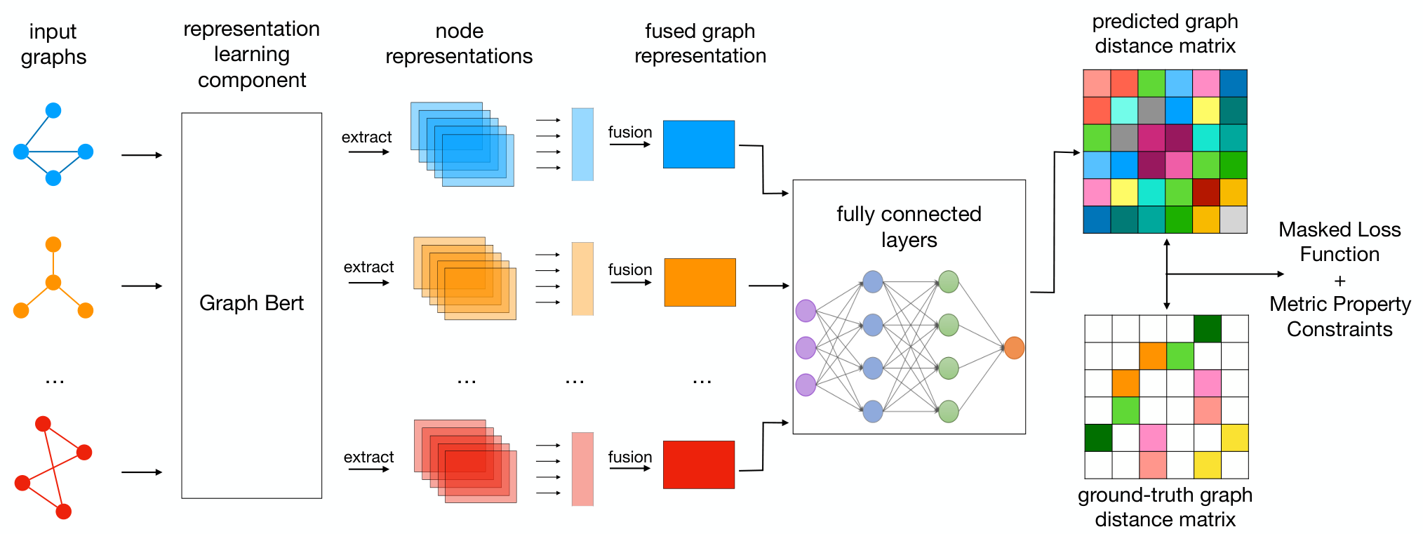
As illustrated in Figure 1, given a set of graph instances, e.g., , GB-Distance can effective compute the pairwise distance scores among them with several key functional components:
- •
Graph-Bert Layers: To effectively and efficiently extract the feature representations of the input graph instances, GB-Distance proposes to extend the Graph-Bert model (Zhang et al. 2020) to the graph instance representation learning settings. Different from the existing graph neural networks, Graph-Bert learns node representations merely based on the attention mechanisms, which will not suffer from the common performance problems with the existing graph neural networks. Also GB-Distance can be pre-trained in an unsupervised manner, which can greatly lower down the time costs for model learning.
- •
Representation Fusion: In addition, different from the target node representation learning (Zhang et al. 2020), in this paper, we focus on learning the representations of graph instances instead. In GB-Distance, we introduce a fusion component to integrate the learned node representations as the representation of the whole graph instances.
- •
Distance Metric Inference: GB-Distance proposes to apply fully connected layers to compute the distance metrics between pairwise graph instances. Prior to feeding the learned graph instance representations, necessary representation vector comparison operators will also be needed, which is not illustrated in the plot.
- •
Masked Loss Function: GB-Distance doesn’t require a large number of labeled graph pair distance scores as the training data, which can also effectively involve the unlabeled graph pairs in defining the loss function with a mask matrix. Formally, in the masked loss function, the labeled and unlabeled graph pairs will be assigned with different weights.
- •
Metric Property based Constraints: The graph distance metric properties, including non-negativity, identity of indiscernibles, symmetry and triangle inequality, will introduce different mathematical constraints (or involved as a functional components) to define the final objective function. GB-Distance will learn both the model variables, graph representations, and their pairwise distance metric scores by optimizing the objective function. Necessary model pre-training will be adopted in GB-Distance as well so as to lower down the learning time costs. Furthermore, to handle the triangle inequality constraints, we will introduce a post-process algorithm to resolve the violations in the learned results.
Detailed information about these five functional components in GB-Distance will be introduced in detail in the following subsections.
4.2 Graph-Bert based Layers and Pre-Training
In this part, we will talk about the graph representation learning layer used in GB-Distance, which can compute the node-order-invariant graph representations effectively. Formally, given an input graph instance , we can denote its node set as (here, we will not indicate the graph instance index for representation simplicity). The relative node positions in the list will not change the nodes’ learned representations in GB-Distance. Therefore, for presentation simplicity, regardless of the node orders, we can also serialize the nodes into a list as .
For each node in the list, e.g., , we can represent its raw features as a vector as defined in Section 3, which may cover various types of information, e.g., node tags, attributes, textual descriptions and even images. Via certain embedding functions, we can denote the embedded feature representation of ’s raw features as
| (1) |
Here, the embedded feature vector and denotes its vector length. Meanwhile, depending on the input features, different approaches can be utilized to define the function, e.g., CNN for image features, LSTM for textual features, positional embedding for tags and MLP for real-number features.
In addition to the node raw feature embedding, we also define the nodes’ Weisfeiler-Lehman role embedding vector in this paper, which effectively denotes the nodes’ global roles in the input graph. As introduced in (Zhang et al. 2020), nodes’ Weisfeiler-Lehman code is node-order-invariant, which denotes a positional property of the nodes actually. Formally, given a node in the input graph instance, we can denote its pre-computed WL code as , whose corresponding embeddings can be represented as
| (2) | ||||
where and denotes the vector index .
Both the node raw attribute embedding and WL role embedding are inherit from (Zhang et al. 2020). Meanwhile, to handle the graph instances without node attributes, we also introduce two new embeddings based on the nodes’ fix-order neighborhood and nodes’ degrees, which can be denoted as follows
| (3) | ||||
where denotes the connection weights between and the other nodes in the graph and is the degree of . To ensure vector is node-order invariant, we cast an artificial fixed node order for the vector entries. In addition, for all the nodes in the identical graph, such an artificial node order will be the same.
By aggregating the above four embedding vectors together, we can define the initial input embeddings for node as
| (4) |
Among all the graphs in , we can represent the largest graph instance size as . Furthermore, the initial embedding vectors of all the nodes in graph can be organized as a matrix . For the graph instances with less than nodes, we will adopt zero padding to expand the matrix to the dimensions specified above.
GB-Distance uses the graph-transformer based encoder to update the nodes’ representations iteratively with multiple layers ( layers) iteratively as follows:
| (5) |
Operator denotes the graph-transformer, whose concrete representation can be illustrated as follows:
| (6) | ||||
where
| (7) |
In the above equations, are the involved variables. To simplify the presentations in the paper, we assume nodes’ hidden vectors in different layers have the same length. Notation represents the graph residual term introduced in (Zhang & Meng 2019). Different from the original Graph-Bert in (Zhang et al. 2020), which forces to add the residual terms of the target to all the nodes in the sub-graphs, the residual terms used here correspond to all the nodes in the graph instance instead.
Furthermore, the operator will aggregate such learned nodes’ representations to define the representation of the graph instances. Formally, we can rewrite such an operator as follows:
| (8) |
In this paper, we use the simple node representation averaging to define the fusion component for graph instance representation learning. Finally, vector will be outputted as the learned representation of the input graph instance . Meanwhile, to ensure such learned representations can capture the graph information, in this paper, we also propose to pre-train the Graph-Bert layer in advance with the node raw attribute reconstruction and graph structure recovery tasks concurrently as introduced in (Zhang et al. 2020). These two pre-training task both work in an unsupervised learning manner, and the pre-training time cost is only decided by the available graph instance numbers, which is very minor compared against the graph pairwise distance metric optimization to be discussed later. The pre-training allows GB-Distance to initialize the graph-transformer layers with a good state, which will greatly lower down the learning cost GB-Distance greatly afterwards.
4.3 Distance Metric Inference
Based on the above descriptions, we can denote the learned representations for all the graph instances in as set . GB-Distance can effective project the graph instance pairs to their corresponding distance metric values with several fully connected (FC) layers. Formally, given an input graph pair and , we can represent their fused representations as and , respectively. The distance between them can be inferred effectively in GB-Distance as follows:
| (9) |
where denotes the entry-wise square of the input vector and represents the fully connected layers. To ensure the learned distance metric is symmetric, we compute in the model instead of simple vector concatenation. Meanwhile, for the output layer in , function is adopted to ensure the learned distance metric value is non-negative and within a normalized range . According to the above definition, it is easy to know that the identity of indiscernibles property can be effectively maintained, as holds for .
Based on the inference model, we can represent the pairwise graph distance metric values as a matrix ( denotes the graph instance set size), where entry . According to the above model description, we can know that matrix is symmetric since holds for any graph pairs. Meanwhile, based on the graph true distance metric (which will be introduced in Section 5 in detail), for the graph pairs in the training set, we can represent them as the ground-truth matrix , where the diagonal entries are assigned with value (to denote they are extremely close or identical) and entries corresponding to the unlabeled graph pairs are filled in with value by default (to denote they are far away). To effectively incorporate both the labeled and unlabeled graph pairs in the model learning, we introduce the masked loss function as follows:
| (10) |
where denotes the matrix norm and denotes the mask matrix with entry
| (11) |
In the above equation, is a hyper-parameter which can be fine-tuned with the validation set, and is usually a very large number (e.g., ) to force the identity of indiscernibles property can hold.
4.4 Metric Property based Constraints
In the above model architecture introduction, we have accommodated the function components to incorporate several key properties of the distance metric, including symmetry (in Equation 9), non-negativity (with the function for the output layer in operator), and identity of indiscernibles (in both Equation 9 and Equation 11), respectively. Here, we will tackle the last important property on the distance metric, i.e., triangle inequality.
Formally, for the distance metric , we can represent the triangle inequality on any three graph instances with the following equation:
| (12) |
If we represent such constraints based on the distance matrix to be inferred, it can be denoted as
| (13) |
Based on it, we can represent the overall framework objective function of the graph neural distance metric learning problem as follows:
| (14) | ||||
where both the model variables and the distance matrix variable are to be optimized concurrently.
4.5 Practical Issues in Framework Learning
To learn the mode, we can denote as the collection of all potential distance matrices which can meet the constraints. As inspired by (Sra et al. 2005), we can prove that the objective function is learnable, and its global optimum can also be identified subject to certain conditions with the following theorem.
while () do
, ,
end for
Return end
| Methods | Datasets | ||||||||
| AIDS | LINUX | IMDB | |||||||
| p@10 | p@10 | p@10 | |||||||
| GED* (Riesen et al. 2013) | 1.000* | 1.000* | 1.000* | 1.000* | 1.000* | 1.000* | NA | NA | NA |
| Beam (Neuhaus et al. 2006) | 0.609 | 0.463 | 0.481 | 0.827 | 0.714 | 0.973 | - | 0.837* | 0.803* |
| VJ (Fankhauser et al. 2011) | 0.517 | 0.383 | 0.310 | 0.581 | 0.450 | 0.287 | - | 0.872* | 0.825* |
| Hungarian (Riesen & Bunke 2009) | 0.510 | 0.378 | 0.360 | 0.638 | 0.517 | 0.913 | - | 0.874* | 0.815* |
| HED (Fischer et al. 2015) | - | 0.469 | 0.386 | - | 0.801 | 0.982 | - | 0.627 | 0.801 |
| EmbAvg (Defferrard et al. 2016) | - | 0.455 | 0.176 | - | 0.012 | 0.071 | - | 0.179 | 0.233 |
| GCNMean (Defferrard et al. 2016) | - | 0.501 | 0.186 | - | 0.424 | 0.141 | - | 0.307 | 0.200 |
| GCNMax (Defferrard et al. 2016) | - | 0.480 | 0.195 | - | 0.495 | 0.437 | - | 0.342 | 0.425 |
| Siamese MPNN (Riba et al. 2018) | - | 0.210 | 0.032 | - | 0.024 | 0.009 | - | 0.093 | 0.023 |
| GB-Distance | 0.551 | 0.440 | 0.226 | 0.613 | 0.534 | 0.332 | 0.636 | 0.515 | 0.242 |
| GB-Distance (Triangle Fixing) | 0.618 | 0.485 | 0.395 | 0.654 | 0.602 | 0.516 | 0.632 | 0.514 | 0.250 |
Theorem 1
Given the collection of all potential distance matrices , the objective function can always attain its minimum on . Moreover, every local minimum is a global minimum. If, in addition, the norm is strictly convex and the weight matrix has no zeros or infinities off its diagonal, then there is a unique global minimum.
The main task to prove the theorem is to show that the objective function has no directions of recession, so it must attain a finite minimum on . Due to the limited space, we will not provide its proof here. If the readers are interested in the proof, you may also refer to (Sra et al. 2005) for more detailed information.
The main challenge in learning the framework lies in the constraints introduced by the triangle inequality property on the distance metric, which will render the neural network very challenging to optimize. In this paper, we propose to train the model and obtain the final inferred distance matrix with two phases instead.
Step 1: Unconstrained Model Training Without considering the constraints, we can define the objective function in model learning as the following objective function:
| (15) |
Meanwhile, to lower down the learning cost, the Graph-Bert component involved in GB-Distance can also be pre-trained in advance as discussed in Section 4.2. Formally, based on the learned model, we can denote the inferred graph pairwise distance matrix as , where the entries of the training instances are over-written with their true distance values.
Step 2: Constrained Metric Refining Based on the real-number distance matrix, we can denote the constrained metric refining objective function as follows:
| (16) | ||||
Distinct from Equations 14 and 15, term in the above equation is a constant matrix (not a variable any more). The only variable to be optimized in the above equation is , which actually can be reduced to the metric nearness problem as studied in (Sra et al. 2005). In this paper, we will take the norm to define the loss function, and will use the triangle fixing algorithm as illustrated in Algorithm 1 to help refine the learned distance metric values among the graph pairs. Formally, the output results of the triangle fixing algorithms will be returned as the final result.
5 Experiments
In this section, extensive experiments will be done on real-world benchmark datasets to test the effectiveness of GB-Distance proposed in this paper.
5.1 Dataset and Experimental Settings
Dataset Descriptions: The datasets used in this paper include AIDS (Zeng et al. 2009; Wang et al. 2012; Zhao et al. 2013; Zheng et al. 2013; Liang & Zhao 2017), LINUX (Wang et al. 2012) and IMDB (Yanardag & Vishwanathan 2015), which are all the benchmark datasets used in existing graph similarity search papers. For the AIDS and LINUX datasets (with small sized graphs), we will use the graph edit distance (GED) (Riesen et al. 2013) as the ground truth; where as the ground truth of IMDB (graph instances in IMDB is much larger and their graph edit distance cannot be computed any more), we will compute the average of the graph pairwise Beam distance (Neuhaus et al. 2006), VJ distance (Fankhauser et al. 2011), and Hungarian distance (Riesen & Bunke 2009) as the ground truth. To be more precise, the graph pairwise true distance between graph and is defined as , where denotes the result computed by GED or the average of Beam, VJ and Hungarian as mentioned above.
Experimental Settings: For each dataset, the graph instances are partition into the train, validation and test sets according to the ratios: 6:2:2. Pairwise graph distance values will be computed for the graph instances in the training set; whereas the pairwise graphs between the those in the validation set and training set will be used to tune the model parameters. The final testing results are achieved for the pairwise graph instances between those from the testing set and the graphs in the whole dataset.
Comparison Methods: The comparison methods used in this paper include both classic combinatorial optimization based algorithms, e.g., Beam (Neuhaus et al. 2006), Volgenant-Jonker (VJ) (Fankhauser et al. 2011), Hungarian (Riesen & Bunke 2009) and Hausdorff Edit Distance (HED) (Fischer et al. 2015), and the recent deep neural network based graph distance algorithms, e.g., Message Passing Neural Networks (MPNN) (Riba et al. 2018), EmbAvg, GCN-Mean, and GCN-Max (Defferrard et al. 2016). The evaluation metrics adopted in this paper include Spearman’s Rank Correlation Coefficient (), Kendall’s Rank Correlation Coefficient (), and Precision@10.
Default Parameter Settings: If not specified, the GB-Distance model used in this paper will have the following default parameter settings: input portal size: (AIDS and LINUX) and (IMDB); hidden size: 32; attention head number: 2; hidden layer number: ; learning rate: 0.001; weight decay: ; intermediate size: 32; hidden dropout rate: 0.5; attention dropout rate: 0.3; graph residual term: raw or none; training epoch: 1000 (early stop when necessary).
5.2 Experimental Results
Main Results: The main results achieved by GB-Distance and the other baseline methods on the three benchmark datasets are provided in Table 1. Considering that GED and Beam/VJ/Hungarian are used to compute the ground truth on the AIDS/LINUX and IMDB, respectively, the evaluation scores obtained by these on the datasets (the scores are highlighted with *) are much better than the remaining methods. According to the table, since Beam is a fast approximated algorithm for computing the graph edit distance, its learning results are highly similar to the ground truth computed by the GED method on the AIDS and LINUX datasets. Meanwhile, among all the deep learning and graph neural network based distance metrics, GB-Distance and GB-Distance (Triangle Fixing) can out-perform them with great advantages. For these three studied datasets, GB-Distance and GB-Distance (Triangle Fixing) can rank among the top 3 for most of the evaluation metrics, which are highlighted in a bolded font in the table.
With vs Without Triangle Inequality Constraint: According to Table 1, for the GB-Distance method with the triangle inequality fixing process, it can improve the learning performance greatly on both AIDS and LINUX. Meanwhile, for the IMDB dataset, involving the triangle inequality fixing doesn’t change the learning performance. Partial reason can be that instances in IMDB is relatively larger, which can provide more information to learn distinguishable representations. Further refining the learning results with the triangle fixing will not change most of the graph pairwise distance scores.
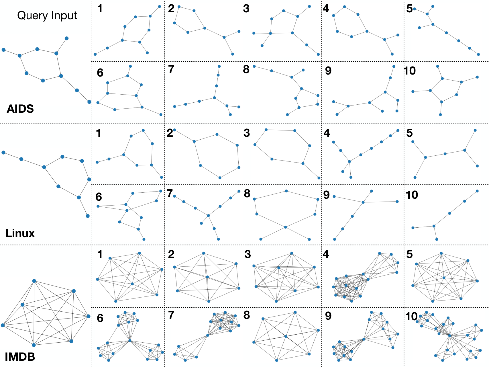
Case Studies: As illustrated in Figure 2, we also show the top 10 graph instances in the datasets which has the shortest distance computed by GB-Distance to the input query graph. According to the results, GB-Distance can effectively identify the graph instances with similar structures to the input graph instance. For instance, the top 1 graph instance identified by GB-Distance on these three datasets all have the identical structure as the query graph input. Meanwhile, the remaining graph instances in the top 10 list also have very similar structures as the input graph.
6 Conclusion
In this paper, we have studied the semi-supervised graph distance metric learning problem. To address the problem, a novel graph neural distance metric, i.e., GB-Distance, have been introduced. GB-Distance learns the graph instance representations by extending Graph-Bert to the new problem settings, which can also be pre-trained in advance to lower-down the overall optimization time costs. In the learning process, the basic distance metric properties, i.e., non-negative, identity of indiscernibles, symmetry and triangle inequality, are all maintained, which can differentiate GB-Distance from most of the existing graph distance metric learning works. Extensive experiments done on real-world graph benchmark datasets also demonstrate the effectiveness of GB-Distance especially compared with the existing graph neural network based baseline methods.
References
- Bai et al. (2019) Bai, Y., Ding, H., Bian, S., Chen, T., Sun, Y., and Wang, W. Simgnn: A neural network approach to fast graph similarity computation. In Proceedings of the Twelfth ACM International Conference on Web Search and Data Mining, pp. 384–392, 2019.
- Bullmore & Bassett (2011) Bullmore, E. and Bassett, D. Brain graphs: graphical models of the human brain connectome. Annual review of clinical psychology, 2011.
- Bunke (1997) Bunke, H. On a relation between graph edit distance and maximum common subgraph. Pattern Recogn. Lett., 1997.
- Bunke & Shearer (1998) Bunke, H. and Shearer, K. A graph distance metric based on the maximal common subgraph. Pattern Recogn. Lett., 1998.
- Chung et al. (2014) Chung, J., Gülçehre, Ç., Cho, K., and Bengio, Y. Empirical evaluation of gated recurrent neural networks on sequence modeling. CoRR, abs/1412.3555, 2014. URL http://arxiv.org/abs/1412.3555.
- Defferrard et al. (2016) Defferrard, M., Bresson, X., and Vandergheynst, P. Convolutional neural networks on graphs with fast localized spectral filtering. CoRR, abs/1606.09375, 2016. URL http://arxiv.org/abs/1606.09375.
- Devlin et al. (2018) Devlin, J., Chang, M., Lee, K., and Toutanova, K. BERT: pre-training of deep bidirectional transformers for language understanding. CoRR, abs/1810.04805, 2018. URL http://arxiv.org/abs/1810.04805.
- Duvenaud et al. (2015) Duvenaud, D., Maclaurin, D., Iparraguirre, J., Bombarell, R., Hirzel, T., Aspuru-Guzik, A., and Adams, R. Convolutional networks on graphs for learning molecular fingerprints. In NIPS. 2015.
- Fankhauser et al. (2011) Fankhauser, S., Riesen, K., and Bunke, H. Speeding up graph edit distance computation through fast bipartite matching. In Proceedings of the 8th International Conference on Graph-Based Representations in Pattern Recognition, GbRPR?11, pp. 102?111, Berlin, Heidelberg, 2011. Springer-Verlag. ISBN 9783642208430.
- Fischer et al. (2015) Fischer, A., Suen, C. Y., Frinken, V., Riesen, K., and Bunke, H. Approximation of graph edit distance based on hausdorff matching. Pattern Recogn., 48(2):331?343, February 2015. ISSN 0031-3203. doi: 10.1016/j.patcog.2014.07.015. URL https://doi.org/10.1016/j.patcog.2014.07.015.
- Gao et al. (2010) Gao, X., Xiao, B., Tao, D., and Li, X. A survey of graph edit distance. Pattern Anal. Appl., 2010.
- Hochreiter & Schmidhuber (1997) Hochreiter, S. and Schmidhuber, J. Long short-term memory. Neural Comput., 9(8), November 1997.
- Hu et al. (2009) Hu, X., Chiueh, T., and Shin, K. Large-scale malware indexing using function-call graphs. In CCS, 2009.
- Huang & Carley (2019) Huang, B. and Carley, K. M. Inductive graph representation learning with recurrent graph neural networks. CoRR, abs/1904.08035, 2019. URL http://arxiv.org/abs/1904.08035.
- Jin et al. (2018) Jin, W., Barzilay, R., and Jaakkola, T. Junction tree variational autoencoder for molecular graph generation. CoRR, abs/1802.04364, 2018.
- Kim (2014) Kim, Y. Convolutional neural networks for sentence classification. In Proceedings of the 2014 Conference on Empirical Methods in Natural Language Processing (EMNLP), pp. 1746–1751, Doha, Qatar, October 2014. Association for Computational Linguistics. doi: 10.3115/v1/D14-1181. URL https://www.aclweb.org/anthology/D14-1181.
- Kipf & Welling (2016) Kipf, T. N. and Welling, M. Semi-supervised classification with graph convolutional networks. CoRR, abs/1609.02907, 2016.
- Kondor & Pan (2016) Kondor, R. and Pan, H. The multiscale laplacian graph kernel, 2016.
- Li et al. (2018) Li, Q., Han, Z., and Wu, X. Deeper insights into graph convolutional networks for semi-supervised learning. CoRR, abs/1801.07606, 2018.
- Li et al. (2019) Li, Y., Gu, C., Dullien, T., Vinyals, O., and Kohli, P. Graph matching networks for learning the similarity of graph structured objects. CoRR, abs/1904.12787, 2019.
- Liang & Zhao (2017) Liang, Y. and Zhao, P. Similarity search in graph databases: A multi-layered indexing approach. pp. 783–794, 04 2017. doi: 10.1109/ICDE.2017.129.
- Lin et al. (2019) Lin, G., Wang, J., Liao, K., Zhao, F., and Chen, W. Structure fusion based on graph convolutional networks for semi-supervised classification. CoRR, abs/1907.02586, 2019. URL http://arxiv.org/abs/1907.02586.
- Meng & Zhang (2019) Meng, L. and Zhang, J. Isonn: Isomorphic neural network for graph representation learning and classification. CoRR, abs/1907.09495, 2019. URL http://arxiv.org/abs/1907.09495.
- Neuhaus et al. (2006) Neuhaus, M., Riesen, K., and Bunke, H. Fast suboptimal algorithms for the computation of graph edit distance. In Yeung, D.-Y., Kwok, J. T., Fred, A., Roli, F., and de Ridder, D. (eds.), Structural, Syntactic, and Statistical Pattern Recognition, pp. 163–172, Berlin, Heidelberg, 2006. Springer Berlin Heidelberg. ISBN 978-3-540-37241-7.
- Riba et al. (2018) Riba, P., Fischer, A., Lladós, J., and Fornés, A. Learning graph distances with message passing neural networks. In 2018 24th International Conference on Pattern Recognition (ICPR), pp. 2239–2244, Aug 2018. doi: 10.1109/ICPR.2018.8545310.
- Richiardi et al. (2013) Richiardi, J., Achard, S., Bunke, H., and Van De Ville, D. Machine learning with brain graphs: Predictive modeling approaches for functional imaging in systems neuroscience. IEEE Signal Processing Magazine, 2013.
- Riesen & Bunke (2009) Riesen, K. and Bunke, H. Approximate graph edit distance computation by means of bipartite graph matching. Image Vision Comput., 27(7):950?959, June 2009. ISSN 0262-8856. doi: 10.1016/j.imavis.2008.04.004. URL https://doi.org/10.1016/j.imavis.2008.04.004.
- Riesen et al. (2013) Riesen, K., Emmenegger, S., and Bunke, H. A novel software toolkit for graph edit distance computation. In Kropatsch, W. G., Artner, N. M., Haxhimusa, Y., and Jiang, X. (eds.), Graph-Based Representations in Pattern Recognition, pp. 142–151, Berlin, Heidelberg, 2013. Springer Berlin Heidelberg. ISBN 978-3-642-38221-5.
- Shervashidze et al. (2009) Shervashidze, N., Vishwanathan, S., Petri, T., Mehlhorn, K., and Borgwardt, K. Efficient graphlet kernels for large graph comparison. In van Dyk, D. and Welling, M. (eds.), Proceedings of the Twelth International Conference on Artificial Intelligence and Statistics, volume 5 of Proceedings of Machine Learning Research, pp. 488–495, Hilton Clearwater Beach Resort, Clearwater Beach, Florida USA, 16–18 Apr 2009. PMLR. URL http://proceedings.mlr.press/v5/shervashidze09a.html.
- Sra et al. (2005) Sra, S., Tropp, J., and Dhillon, I. Triangle fixing algorithms for the metric nearness problem. In Saul, L. K., Weiss, Y., and Bottou, L. (eds.), Advances in Neural Information Processing Systems 17. 2005.
- Sun et al. (2019) Sun, K., Lin, Z., and Zhu, Z. Adagcn: Adaboosting graph convolutional networks into deep models, 2019.
- Togninalli et al. (2019) Togninalli, M., Ghisu, M. E., Llinares-López, F., Rieck, B., and Borgwardt, K. M. Wasserstein weisfeiler-lehman graph kernels. CoRR, abs/1906.01277, 2019. URL http://arxiv.org/abs/1906.01277.
- Vaswani et al. (2017) Vaswani, A., Shazeer, N., Parmar, N., Uszkoreit, J., Jones, L., Gomez, A. N., Kaiser, L., and Polosukhin, I. Attention is all you need. CoRR, abs/1706.03762, 2017. URL http://arxiv.org/abs/1706.03762.
- Veličković et al. (2018) Veličković, P., Cucurull, G., Casanova, A., Romero, A., Liò, P., and Bengio, Y. Graph Attention Networks. International Conference on Learning Representations, 2018.
- Wang et al. (2012) Wang, X., Ding, X., Tung, A., Ying, S., and Jin, H. An efficient graph indexing method. Proceedings - International Conference on Data Engineering, 04 2012. doi: 10.1109/ICDE.2012.28.
- Wikipedia (2019) Wikipedia. Metric (mathematics). https://en.wikipedia.org/wiki/Metric_(mathematics), 2019. [Online; accessed 15-October-2019].
- Wu et al. (2019) Wu, Z., Pan, S., Chen, F., Long, G., Zhang, C., and Yu, P. S. A comprehensive survey on graph neural networks. CoRR, abs/1901.00596, 2019. URL http://arxiv.org/abs/1901.00596.
- Xing et al. (2003) Xing, E. P., Jordan, M. I., Russell, S. J., and Ng, A. Y. Distance metric learning with application to clustering with side-information. In Becker, S., Thrun, S., and Obermayer, K. (eds.), Advances in Neural Information Processing Systems 15, pp. 521–528. MIT Press, 2003.
- Yan & Han (2002) Yan, X. and Han, J. gspan: graph-based substructure pattern mining. In ICDM, 2002.
- Yanardag & Vishwanathan (2015) Yanardag, P. and Vishwanathan, S. Deep graph kernels. In Proceedings of the 21th ACM SIGKDD International Conference on Knowledge Discovery and Data Mining, KDD ?15, pp. 1365?1374, New York, NY, USA, 2015. Association for Computing Machinery. ISBN 9781450336642. doi: 10.1145/2783258.2783417. URL https://doi.org/10.1145/2783258.2783417.
- Yang & Jin (2006) Yang, L. and Jin, R. Distance metric learning: A comprehensive survey. Michigan State Universiy, 2, 2006.
- Ying & Li (2012) Ying, Y. and Li, P. Distance metric learning with eigenvalue optimization. J. Mach. Learn. Res., 13(null):1?26, January 2012. ISSN 1532-4435.
- Zeng et al. (2009) Zeng, Z., Tung, A. K. H., Wang, J., Feng, J., and Zhou, L. Comparing stars: On approximating graph edit distance. Proc. VLDB Endow., 2(1):25?36, August 2009. ISSN 2150-8097. doi: 10.14778/1687627.1687631. URL https://doi.org/10.14778/1687627.1687631.
- Zhang (2019) Zhang, J. Graph neural networks for small graph and giant network representation learning: An overview, 2019. URL https://arxiv.org/abs/1908.00187.
- Zhang & Meng (2019) Zhang, J. and Meng, L. Gresnet: Graph residual network for reviving deep gnns from suspended animation. ArXiv, abs/1909.05729, 2019. URL https://arxiv.org/abs/1909.05729.
- Zhang et al. (2020) Zhang, J., Zhang, H., Xia, C., and Sun, L. Graph-bert: Only attention is needed for learning graph representations, 2020. URL https://arxiv.org/abs/2001.05140.
- Zhao et al. (2013) Zhao, X., Xiao, C., Lin, X., Liu, Q., and Zhang, W. A partition-based approach to structure similarity search. Proc. VLDB Endow., 7(3):169?180, November 2013. ISSN 2150-8097. doi: 10.14778/2732232.2732236. URL https://doi.org/10.14778/2732232.2732236.
- Zheng et al. (2013) Zheng, W., Zou, L., Lian, X., Wang, D., and Zhao, D. Graph similarity search with edit distance constraint in large graph databases. In Proceedings of the 22nd ACM International Conference on Information & Knowledge Management, CIKM ?13, pp. 1595?1600, New York, NY, USA, 2013. Association for Computing Machinery. ISBN 9781450322638. doi: 10.1145/2505515.2505723. URL https://doi.org/10.1145/2505515.2505723.