Stationary quantum entanglement between a massive mechanical membrane
and a low frequency LC circuit

In optomechanics, an optical field can couple to a massive mechanical oscillator (MO) via the radiation pressure force omRMP. This approach provides the possibility to prepare quantum states of macroscopic systems by manipulating optical degrees of freedom. Over the past decade, significant experimental progress has been achieved in observing quantum effects in massive mechanical systems, including reaching the quantum ground state ground1; ground2, quantum squeezing of the mechanical motion sqz1; sqz2; sqz3, quantum entanglement between two MOs enMM1; enMM2, and between a MO and an electromagnetic field enOM1; enOM2, among many others. Such quantum states of massive objects have important implications for both quantum technologies, e.g., quantum sensing sensing, quantum transducers SG, as well as foundational studies of decoherence theories at the macro scale and the boundary between the quantum and classical worlds review.

In this paper, we provide a scheme to entangle a massive MO with a macroscopic low-frequency LC oscillator. Specifically, we consider a tripartite system where a mechanical membrane is capacitively coupled to an LC resonator and further optomechanically coupled to an optical cavity. Unlike most other approaches with GHz resonators ground1; enOM1; Lehnert; Fink, the LC resonator we consider here is in the radio frequency domain, around 1 MHz Polzik14; Iman18, and close to the mechanical frequency. Such a low-frequency LC resonator means a much larger product $L\times C$ ($L$-inductance; $C$-capacitance) than that at microwave frequency ($10^{6}$ larger for frequency of 1 MHz compared to 1 GHz), which typically implies a much larger number of charges and a much bigger LC circuit. The membrane-LC interaction takes a nonlinear form $H_{int}=\hbar g_{0}xq^{2}$ DV07; DV11; Polzik11, where $x$ is the mechanical position, $q$ the charge and $g_{0}$ the bare electro-mechanical coupling rate, which is a radiation pressure-like interaction. We note that the entanglement between a nanomechanical resonator and an LC resonator of microwave frequency has been well studied DV07; DV11, where the electro-mechanical interaction is a radiation pressure type $\propto g_{0}xb^{{\dagger}}b$. Here $b$ is the annihilation operator of the LC field and $q=(b+b^{{\dagger}})/\sqrt{2}$. The interaction is derived by taking the rotating wave approximation (RWA) and neglecting fast oscillating terms, which is valid only for the LC frequency much larger than the mechanical frequency, $\omega_{LC}\gg\omega_{m}$. Such a radiation pressure interaction predicts the generation of electro-mechanical entanglement if an appropriate microwave drive is adopted DV07. However, when the LC frequency is approaching the mechanical frequency, like in Ref. Polzik14; Iman18 and as considered here, it is not clear how to apply an appropriate driving field such that (stationary) electro-mechanical entanglement can be produced. In other words, it is not apparent how to apply the mechanism of Ref. DV07 to two nearly resonant low-frequency oscillators.

Inspired by recent experiments Polzik14; Iman18, we apply a DC drive for the LC circuit, which significantly enhances the effective electro-mechanical coupling rate. The linearized interaction takes the form $\propto g\delta x\delta q$ Polzik11; Polzik14, where $g$ is the effective coupling rate. Based on this “quadrature-quadrature” coupling, electro-mechanical entanglement can indeed be created, but only at unrealistic extremely low temperature (below 0.1 mK for 1 MHz oscillators), where both the oscillators are actually at their quantum ground state. In this situation, the component of the beamsplitter interaction in the “quadrature-quadrature” coupling is significantly suppressed, while the component of the two-mode squeezing interaction plays a dominate role, leading to the generation of electro-mechanical entanglement. The entanglement completely vanishes at typical cryogenic temperatures of a few tens of millikelvin, because of the low resonant frequencies and thus large thermal occupations. In our approach, we overcome this limitation and show that by further coupling the mechanical membrane to an optical cavity field via radiation pressure, and by driving the cavity with a red-detuned laser, both the mechanical and electrical modes get significantly cooled, which leads to the emergence of electro-mechanical entanglement. Here, the red-detuned cavity cools the mechanical mode, which then acts as a cold bath for the electrical mode LCcooling. The entanglement is in the steady state regime and robust against temperature.

The remainder of the paper is organized as follows: in Sec. II, we introduce our tripartite opto-electro-mechanical system, provide its Hamiltonian and the corresponding Langevin equations, and in Sec. III we show how to obtain the steady-state solutions of the system and quantify the entanglement. In Sec. IV, we present the results of electro-mechanical entanglement and discuss optimal parameter regimes for obtaining the entanglement and its detection. Finally, we draw the conclusions in Sec. V.

We consider a tripartite opto-electro-mechanical system, as shown in Fig. 1, which consists of an LC electrical circuit, a MO, and an optical cavity. An experimental realization of a suitable MO could be a metal coated nanomembrane Polzik14; Iman18, which is capacitively coupled to an LC resonator and further coupled to an optical cavity field via radiation pressure. Specifically, the radiation pressure of the cavity field causes a mechanical displacement which further changes the capacitance of the LC circuit, and conversely, the voltage fluctuation in the LC circuit leads to an optical phase shift via the mediation of the MO. The Hamiltonian of the system reads

where $a$ ($a^{{\dagger}}$) is the annihilation (creation) operator of the cavity mode, $x$ and $p$ ($q$ and $\phi$) are the dimensionless position and momentum (charge and flux) quadratures of the mechanical (LC) resonator, and therefore $[a,a^{{\dagger}}]\,{=}\,1$ and $[x,p]\,{=}\,[q,\phi]\,{=}\,i$. The resonance frequencies $\omega_{c}$, $\omega_{m}$, and $\omega_{LC}\,{=}\,\frac{1}{\sqrt{LC}}$ are of the cavity, mechanical, and LC resonators, respectively, where $L$ ($C$) is the inductance (capacitance) of the LC circuit. The capacitance $C(x)$ is a function of the mechanical position $x$, which characterizes the capacitive coupling to the MO. The MO-LC nonlinear coupling $\propto g_{0}xq^{2}$ is derived by expanding the capacitance $C(x)$ around the membrane equilibrium position and expanding the capacitive energy $\frac{q^{2}}{2C(x)}$ as a Taylor series up to first order DV07; Polzik11, and $G_{0}$ is the single-photon optomechanical coupling rate. The last two terms in the Hamiltonian denote the electric driving for the LC circuit and the laser driving for the cavity, respectively, where $V$ is a DC bias voltage (see Fig. 1 (a)), $q_{0}\,{=}\,\sqrt{\hbar/L\omega_{LC}}$ is the zero-point fluctuation of the LC oscillator, and $E=\!\sqrt{2P_{l}\kappa/\hbar\omega_{l}}$ is the coupling between the cavity field with decay rate $\kappa$ and the driving laser with frequency $\omega_{l}$ and power $P_{l}$. Note that Refs. DV07; DV11 considered a different form of MO-LC coupling, $\propto g_{0}xb^{{\dagger}}b$, which was derived by neglecting fast oscillating terms $xbb$ and $xb^{{\dagger}}b^{{\dagger}}$ valid only when $\omega_{LC}\gg\omega_{m}$. Instead, here we consider two low frequency nearly resonant oscillators $\omega_{LC}\simeq\omega_{m}$, and thus one has to consider the full interaction $\propto g_{0}xq^{2}$. Another major difference is that the blue- or red-detuned pump used in Refs. DV07; DV11 to activate electro-mechanical Stokes or anti-Stokes process does not apply, in a clear way, to our case of nearly resonant oscillators.

In the frame rotating at the drive frequency $\omega_{l}$, the quantum Langevin equations (QLEs) governing the system dynamics are given by

where $\Delta_{0}\,\,{=}\,\,\omega_{c}\,{-}\,\omega_{l}$, $\gamma_{m}$ and $\gamma_{LC}\,\,{=}\,\,2R/L$ (with $R$ the resistance of the circuit) are the mechanical and electrical damping rates, respectively, $a^{\rm in}$ is the input noise operator for the cavity, whose mean value is zero and the only non-zero correlation is

The Langevin force operator $\xi$ accounts for the Brownian motion of the MO and is autocorrelated as

where we have made a Markovian approximation valid for large mechanical quality factors $Q_{m}=\omega_{m}/\gamma_{m}\,\,{\gg}\,1$ Markov, and $\bar{n}_{m}\simeq\frac{k_{B}T}{\hbar\omega_{m}}$ is the equilibrium mean thermal phonon number in the high temperature limit, with $k_{B}$ the Boltzmann constant and $T$ the environmental temperature.

In order to get strong optomechanical (electro-mechanical) coupling for cooling both the mechanical and LC oscillators (creating MO-LC entanglement), we consider an intense laser pump, leading to a large amplitude of the cavity field $|\langle a\rangle|\gg 1$, and a large number of charges $\langle q\rangle\gg 1$. This allows us to linearize the system dynamics around the semiclassical averages by writing any operator as $O=\langle O\rangle+\delta O$ ($O\,{=}\,a,x,p,q,\phi$) and neglecting small second-order fluctuation terms. Therefore, the QLEs Eq. (2) are separated into two sets of equations: one is for averages $O_{s}\equiv\langle O\rangle$ and the other for zero-mean quantum fluctuations $\delta O$. The steady-state averages can be obtained by setting the derivatives to zero and solving the following equations

where $\Delta\,\,{=}\,\,\Delta_{0}\,{-}\,G_{0}x_{s}$ is the effective cavity-laser detuning, and $\omega^{\prime}_{LC}=\omega_{LC}+2g_{0}x_{s}$ is the effective LC frequency including the frequency shift caused by the nonlinear MO-LC interaction. The linearized QLEs describing the quadrature fluctuations $(\delta X,\delta Y,\delta x,\delta p,\delta q,\delta\phi)$, with $\delta X=(\delta a+\delta a^{{\dagger}})/\sqrt{2}$, $\delta Y=i(\delta a^{{\dagger}}-\delta a)/\sqrt{2}$, are given by

where $G=\!\sqrt{2}G_{0}a_{s}$ ($g=2g_{0}q_{s}$) is the effective optomechanical (electro-mechanical) coupling rate, and $X^{\rm in}=(a^{\rm in}+a^{\rm in{\dagger}})/\sqrt{2}$, $Y^{\rm in}=i(a^{\rm in{\dagger}}-a^{\rm in})/\sqrt{2}$ are the quadratures of the cavity input noise. Note that in deriving the above QLEs, we have chosen a phase reference such that $a_{s}$ is real and positive. The effective coupling $g$ increases linearly with $q_{s}$, which then is linear dependence on the bias voltage $\bar{V}$ (see Eq. (5)). This means that the electro-mechanical coupling strength can be significantly improved by increasing the bias voltage Polzik14. The fluctuation of the bias voltage $\delta V\,{\equiv}\,V\,{-}\,\bar{V}$ can be considered as the input noise for the flux, and is autocorrelated as

which corresponds to the quantum version of the Johnson-Nyquist noise correlation JN for a resistor $R=\frac{\gamma_{LC}}{2}L$ at temperature $T$ by including the vacuum fluctuation. In such a way, the noise correlation for the operator $\delta{\cal V}(t)\equiv\frac{q_{0}}{\hbar}\delta V(t)$ can be written in the form

with $\bar{n}_{LC}\simeq\frac{k_{B}T}{\hbar\omega_{LC}}$ being the thermal occupancy of the LC oscillator, which takes a consistent form as that for the Langevin force operator $\xi$. This is the reason why we defined the damping rate $\gamma_{LC}$ as twice its conventional definition $\gamma^{\prime}_{LC}=R/L$.

We are interested in the quantum correlation between the mechanical and LC oscillators in the stationary state. Owing to the fact that the dynamics are linearized and all input noises are Gaussian, the Gaussian nature of the state will be preserved for all times. The steady state of the quantum fluctuations of the system is therefore a three-mode Gaussian state and is completely characterized by a $6\times 6$ covariance matrix (CM) ${\cal C}$, which is defined as ${\cal C}_{ij}\,{=}\,\frac{1}{2}\langle u_{i}(t)u_{j}(t^{\prime})+u_{j}(t^{\prime})u_{i}(t)\rangle$ ($i,j\,{=}\,1,2,...,6$), where $u(t)=\big[\delta X(t),\delta Y(t),\delta x(t),\delta p(t),\delta q(t),\delta\phi(t)\big]^{T}$. The stationary CM ${\cal C}$ can be obtained by solving the Lyapunov equation Hahn

where $A$ is the drift matrix determined by the QLEs (6), given by

and $D={\rm diag}\big[\kappa,\,\kappa,\,0,\,\gamma_{m}(2\bar{n}_{m}+1),\,0,\,\gamma_{LC}(2\bar{n}_{LC}+1)\big]$ is the diffusion matrix, which is defined by $\langle n_{i}(t)n_{j}(t^{\prime})+n_{j}(t^{\prime})n_{i}(t)\rangle/2=D_{ij}\delta(t-t^{\prime})$, with the vector of input noises $n(t)\,{=}\,\big[\!\sqrt{2\kappa}X^{\rm in}(t),\!\sqrt{2\kappa}Y^{\rm in}(t),0,\xi(t),0,\delta{\cal V}(t)\big]^{T}$. To quantify the Gaussian entanglement, we adopt the logarithmic negativity LogNeg, which is a full entanglement monotone under local operations and classical communication Plenio and sets an upper bound for the distillable entanglement LogNeg. The logarithmic negativity is defined as Adesso

where $\tilde{\nu}_{-}\,\,{=}\,\min{\rm eig}|i\Omega_{2}\tilde{{\cal C}}_{4}|$ (with the symplectic matrix $\Omega_{2}=\oplus^{2}_{j=1}\!i\sigma_{y}$ and the $y$-Pauli matrix $\sigma_{y}$) is the minimum symplectic eigenvalue of the partially transposed CM $\tilde{{\cal C}}_{4}={\cal P}_{1|2}{{\cal C}_{4}}{\cal P}_{1|2}$, with ${\cal C}_{4}$ being the $4\times 4$ CM of the mechanical and electrical modes, obtained by removing in ${\cal C}$ the rows and columns related to the cavity field, and ${\cal P}_{1|2}={\rm diag}(1,-1,1,1)$ being the matrix that performs partial transposition on CM Simon.

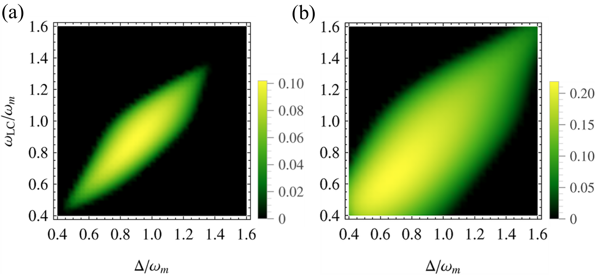
In this section, we present the results of the entanglement between the mechanical and LC oscillators. All results are in the steady state guaranteed by the negative eigenvalues (real parts) of the drift matrix $A$. We adopt experimentally feasible parameters Polzik14; Iman18: $\omega_{c}/2\pi=200$ THz, $\omega_{m}/2\pi=1$ MHz, $\kappa=0.1\omega_{m}$, $\gamma_{m}=10^{-6}\omega_{m}$, $\gamma_{LC}=10^{-5}\omega_{LC}$, and consider the LC frequency $\omega_{LC}$ as a variable which is tuned around $\omega_{m}$. To avoid additional low-frequency electronic noises, LC frequencies much below 1 MHz will not be considered. We work in the resolved sideband limit, $\kappa\ll\omega_{m}$, and assume a relatively large $Q$ factor of the LC oscillator compared to those typically demonstrated at room temperature Polzik14; Iman18 as we place the system at cryogenic temperatures where superconductivity can significantly improve the $Q$ factor Gary. At a few tens of millikelvin, the mechanical and LC oscillators still exhibit significant thermal excitations because of their low frequencies. Therefore, we use a red-detuned laser to drive the cavity and stimulate the optomechanical anti-Stokes process, which results in cooling of the mechanical mode ground2, and owing to the MO-LC coupling, the electrical mode also gets cooled. In such a system, it is even possible to cool a 1 MHz LC resonator into its quantum ground state from temperature of a few tens of millikelvin LCcooling. The cooling process in this hybrid system can be considered as the transport of thermal excitations from the electrical mode to the mechanical mode, and then to the cavity mode, which eventually dissipates the heat via cavity photon leakage to the environment. The low effective temperatures of the mechanical and electrical modes are a precondition for observing their entanglement if strong coupling rates are used. This is verified numerically and shown in Fig. 2, where the entanglement is maximal for a cavity-laser detuning $\Delta\simeq\omega_{LC}$. We assume both the optomechanical and the electro-mechanical coupling to be strong $G,g>\kappa$, in order to significantly cool both the mechanical and electrical modes LCcooling and to ultimately create the desired electro-mechanical entanglement. We have verified that based on the values of the bare coupling rates $G_{0}$ and $g_{0}$ estimated from the experiments Lehnert; Polzik14; Iman18, with the parameters used for our results the nonlinear electro-mechanical coupling induced frequency shift $\omega^{\prime}_{LC}\,{-}\,\omega_{LC}\,{\ll}\,\omega_{LC}$. Therefore, throughout the paper we consider $\omega^{\prime}_{LC}\,{\simeq}\,\omega_{LC}$. Figure 2 also shows that in our system two nearly resonant oscillators are preferred to maximize the entanglement. If the couplings are further increased (cf. Fig. 2(b)) the system becomes unstable for $\Delta\,{<}\,{\sim}\,0.4\omega_{m}$.

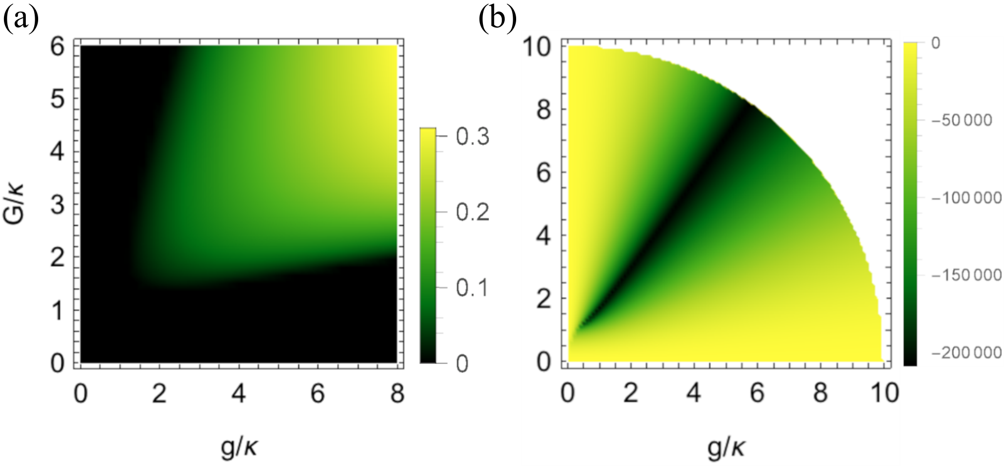
We further show the stationary electro-mechanical entanglement as a function of the two coupling rates $g$ and $G$ for the resonant case Polzik14; Iman18 in Fig. 3(a). It is clear that the entanglement grows with increasing coupling strengths and strong couplings $G,g>\kappa$ are generally required to obtain considerable entanglement. The coupling strengths are restricted by the stability condition. Note that the system becomes stable only when all the eigenvalues of the drift matrix $A$ have negative real parts. The parameter regime where stability occurs can be obtained from the Routh-Hurwitz criterion RH, but the inequalities are quite involved for the present tripartite system. Therefore, to provide an intuitive picture we numerically plot the maximum of the eigenvalues (real parts) of the drift matrix $A$ in Fig. 3(b). The white area denotes that the maximum is larger than zero, i.e., at least one eigenvalue has a positive real part, and thus the system is unstable when the couplings lie within this area. Under such strong couplings, one may conjecture the “optical-spring” effect may play a significant role. We therefore derive the expression of the effective mechanical frequency (see Appendix for the derivation), which in the frequency domain is given by

where the first term is the MO’s natural frequency, and the second term is the frequency shift caused by the optomechanical interaction, followed by the third term which denotes a further frequency shift due to the electro-mechanical coupling. Under the optimal condition for entanglement, $\omega=\Delta=\omega_{m}=\omega_{LC}\equiv\omega_{0}$, and in the resolved sideband limit $\kappa\ll\omega_{m}$, we obtain

For what we have used the strongest coupling $G=6\kappa$ and $\kappa=0.1\omega_{m}$, we have $\omega_{m}^{\rm eff}(\omega_{0})\simeq 0.95\omega_{m}$, implying that the mechanical frequency in most cases remains unchanged. This is mainly due to the fact that we work in the resolved sideband limit omRMP.

We note that the entanglement originates from the component of the two-mode squeezing interaction $\propto g(\delta m\delta b+\delta m^{{\dagger}}\delta b^{{\dagger}})$ in the “quadrature-quadrature” coupling $\propto g\delta x\delta q=g(\delta m+\delta m^{{\dagger}})(\delta b+\delta b^{{\dagger}})/2$, where $m$ is the annihilation operator of the mechanical mode. This can be verified by the fact that there will be no entanglement for a weak coupling $g\ll\omega_{m/LC}$, which allows one to make the RWA and the interaction essentially becomes a beamsplitter type $\propto g(\delta m\delta b^{{\dagger}}+\delta m^{{\dagger}}\delta b)$. As clearly visible from Fig. 3(a), this situation of weak coupling $g<\kappa\ll\omega_{m/LC}$ does not produce any entanglement. Apart from a sufficiently large $g$, $G$ should also be strong, $G>\kappa$, in order to efficiently cool both the oscillators. Taking $G=g=5\kappa$ in Fig. 3(a) for example, we obtain the average excitation number of the two modes: $\bar{n}_{m}^{\rm eff}=\frac{1}{2}\big(\langle\delta x^{2}\rangle+\langle\delta p^{2}\rangle-1\big)\simeq 0.15$; $\bar{n}_{LC}^{\rm eff}=\frac{1}{2}\big(\langle\delta q^{2}\rangle+\langle\delta\phi^{2}\rangle-1\big)\simeq 0.08$, implying both the oscillators are cooled into their quantum ground state. This yields an entanglement $E_{N}\simeq 0.18$.

We further investigate the entanglement as a function of bath temperature and the data in Fig. 4 shows that it is robust against temperature, surviving up to $\sim$100 mK, based on realistic parameters. Even though the electro-mechanical coupling rate $g$ and the $Q$ factor of the LC resonator we use are larger than the demonstrated values Polzik14; Iman18, it is realistic to assume that they can be achieved at low temperature and by properly designing the system Gary.

Finally, we would like to discuss how to detect the electro-mechanical entanglement. The task requires to essentially measure the four quadratures of the mechanical and electrical modes, $(x,p,q,\phi)$, based on which the CM can be re-constructed and the logarithmic negativity can then be computed according to the definition in Eq. (11). To measure the mechanical quadratures, we adopt the strategy used in Refs. enOM1; enOM2; DV07L, i.e., sending a weak red-detuned probe field with detuning equal to the mechanical frequency $\Delta^{p}\simeq\omega_{m}$ into the cavity, which maps the mechanical state onto the anti-Stokes sideband of the probe field at cavity resonance. Thus, by homodyning the probe output field, the two mechanical quadratures are measured. The quadratures of the electrical mode can also be measured by employing a homodyne scheme at radio frequency.

In order to avoid measuring the whole $4\times 4$ CM for quantifying entanglement, alternatively, one can also verify the entanglement by using the Duan criterion Duan, which requires the measurement of only two collective quadratures, $X_{+}=x+q$, and $Y_{-}=p-\phi$. A sufficient condition for entanglement is that the two collective quadratures should satisfy the following inequality

Figure 5 shows that in moderate ranges of temperature and LC $Q$ factor the inequality is fulfilled, indicating the presence of electro-mechanical entanglement. The entanglement survives up to 19 mK for $Q_{LC}=2\times 10^{4}$, and 86 mK for $Q_{LC}=10^{5}$.

We have provided a straightforward but effective approach to preparing entangled states of low-frequency mechanical and LC resonators. At typical cryogenic temperatures, the two resonators still contain significant thermal excitations, which effectively destroy their joint quantum correlations. In order to solve this, we couple the mechanical element to an optical cavity via the radiation pressure force, which can act as an additional cold bath: by drving the cavity with a red-detuned laser, both the mechanical and electrical modes are sequentially cooled, resulting in remarkable electro-mechanical entanglement emerging from thermal noise. The entanglement originates from the electro-mechanical coupling and can be in the stationary state and robust against temperature.

The present work can be considered as a complementary study to the widely explored situation where the LC frequency, typically in microwave domain ground1; enOM1; Lehnert; Fink, is much larger than the mechanical frequency, and in this case electro-mechanical entanglement can be directly generated by adopting an appropriate microwave drive DV07. The entanglement generated in this work, however, uses a different mechanism and is of low-frequency resonators (both around 1 MHz), which implies its macroscopic quantum nature, and would allow us to test quantum theories at a more macroscopic level Bell1; Bell2; Bell3.

We thank D. Vitali and N. Malossi for fruitful discussions and valuable comments on the manuscript, and M. Forsch, I. Marinković, G. Steele, R. Stockill, and A. Wallucks for useful discussions on LC circuits. This project was supported by the European Research Council (ERC StG Strong-Q, 676842) and by the Netherlands Organisation for Scientific Research (NWO/OCW), as part of the Frontiers of Nanoscience program, as well as through a Vidi grant (680-47-541).

Here we show how to derive the effective mechanical frequency in our strongly coupled tripartite system. We solve the QLEs (6) in the frequency domain by taking Fourier transform of each equation and derive the effective mechanical susceptibility, through which we extract the effective mechanical frequency.

Solving separately two quadrature equations for each mode, we obtain the solutions given in terms of the natural susceptibilities of the three subsystems, which are

where $\chi_{c}(\omega)$, $\chi_{m}(\omega)$, and $\chi_{LC}(\omega)$ are the natural susceptibilities of the cavity, mechanical, and electrical modes, respectively, given by

The mutual interactions among the three modes lead to the modification of their natural susceptibilities, and thus yield effective mode frequencies, which are associated to the real part of the reciprocal of the susceptibilities. Inserting $\delta X(\omega)$ and $\delta q(\omega)$ in Eq. (15) into the equation of $\delta x(\omega)$, we obtain

where $\chi_{m}^{\rm eff}(\omega)$ is the effective mechanical susceptibility, defined by

with

where $\chi_{mc}(\omega)$ corresponds to the effective mechanical susceptibility in the presence of only the optomechanical interaction. From the real part of $\chi_{m}^{\rm eff-1}(\omega)$, we extract the effective mechanical frequency, where we can recognize the so-called “optical-spring” effect which is accompanied by a further shift due to the electro-mechanical coupling, i.e.,

References

- (1) M. Aspelmeyer, T. J. Kippenberg, and F. Marquardt, Rev. Mod. Phys. 86, 1391 (2014).
- (2) J. D. Teufel et al., Nature (London) 475, 359 (2011).
- (3) J. Chan et al., Nature (London) 478, 89 (2011).
- (4) E. E. Wollman et al., Science 349, 952 (2015).
- (5) J.-M. Pirkkalainen et al., Phys. Rev. Lett. 115, 243601 (2015).
- (6) F. Lecocq et al, Phys. Rev. X 5, 041037 (2015).
- (7) R. Riedinger et al., Nature (London) 556, 473 (2018).
- (8) C. F. Ockeloen-Korppi et al., Nature (London) 556, 478 (2018).
- (9) T. A. Palomaki, J. D. Teufel, R. W. Simmonds, and K. W. Lehnert, Science 342, 710 (2013).
- (10) R. Riedinger et al., Nature (London) 530, 313 (2016).
- (11) C. L. Degen, F. Reinhard, and P. Cappellaro, Rev. Mod. Phys. 89, 035002 (2017).
- (12) M. Forsch et al., Nat. Phys. 16, 69 (2020).
- (13) Y. Chen, J. Phys. B 46, 104001 (2013); A. Bassi, K. Lochan, S. Satin, T. P. Singh, and H. Ulbricht, Rev. Mod. Phys. 85, 471 (2013); F. Fröwis, P. Sekatski, W. Dür, N. Gisin, and N. Sangouard, Rev. Mod. Phys. 90, 025004 (2018).
- (14) R. W. Andrews et al., Nat. Phys. 10, 321 (2014).
- (15) S. Barzanjeh et al., Nature 570, 480 (2019).
- (16) T. Bagci et al., Nature (London) 507, 81 (2014).
- (17) I. Moaddel Haghighi, N. Malossi, R. Natali, G. Di Giuseppe, and D. Vitali, Phys. Rev. Applied 9, 034031 (2018).
- (18) D. Vitali, P. Tombesi, M. J. Woolley, A. C. Doherty, and G. J. Milburn, Phys. Rev. A 76, 042336 (2007).
- (19) Sh. Barzanjeh, D. Vitali, P. Tombesi, and G. J. Milburn, Phys. Rev. A 84, 042342 (2011).
- (20) J. M. Taylor, A. S. Sorensen, C. M. Marcus, and E. S. Polzik, Phys. Rev. Lett. 107, 273601 (2011).
- (21) J. Li et al., Ground state cooling of a radio-frequency LC circuit in an optoelectromechanical system. In preparation.
- (22) V. Giovannetti and D. Vitali, Phys. Rev. A 63, 023812 (2001); R. Benguria and M. Kac, Phys. Rev. Lett. 46, 1 (1981).
- (23) J. B. Johnson, Phys. Rev. 32, 97 (1928); H. Nyquist, Phys. Rev. 32, 110 (1928).
- (24) P. C. Parks and V. Hahn, Stability Theory (Prentice Hall, New York, U.S., 1993).
- (25) J. Eisert, Ph.D. thesis, University of Potsdam, Potsdam, Germany, 2001; G. Vidal and R. F. Werner, Phys. Rev. A 65, 032314 (2002).
- (26) M. B. Plenio, Phys. Rev. Lett. 95, 090503 (2005).
- (27) G. Adesso and F. Illuminati, J. Phys. A: Math. Theor. 40, 7821 (2007).
- (28) R. Simon, Phys. Rev. Lett. 84, 2726 (2000).
- (29) M. F. Gely et al., Science 363, 1072 (2019).
- (30) I. S. Gradshteyn and I. M. Ryzhik, Table of Integrals, Series and Products (Academic, Orlando, 1980), Page 1119.
- (31) D. Vitali et al., Phys. Rev. Lett. 98, 030405 (2007).
- (32) L. M. Duan, G. Giedke, J. I. Cirac, and P. Zoller, Phys. Rev. Lett. 84, 2722 (2000).
- (33) S. G. Hofer, K. W. Lehnert, and K. Hammerer, Phys. Rev. Lett. 116, 070406 (2016).
- (34) V. Caprara Vivoli, T. Barnea, C. Galland, and N. Sangouard, Phys. Rev. Lett. 116, 070405 (2016).
- (35) I. Marinković et al., Phys. Rev. Lett. 121, 220404 (2018).