Dynamic Inference: A New Approach Toward Efficient Video Action Recognition
Abstract
Though action recognition in videos has achieved great success recently, it remains a challenging task due to the massive computational cost. Designing lightweight networks is a possible solution, but it may degrade the recognition performance. In this paper, we innovatively propose a general dynamic inference idea to improve inference efficiency by leveraging the variation in the distinguishability of different videos. The dynamic inference approach can be achieved from aspects of the network depth and the number of input video frames, or even in a joint input-wise and network depth-wise manner. In a nutshell, we treat input frames and network depth of the computational graph as a 2-dimensional grid, and several checkpoints are placed on this grid in advance with a prediction module. The inference is carried out progressively on the grid by following some predefined route, whenever the inference process comes across a checkpoint, an early prediction can be made depending on whether the early stop criteria meets. For the proof-of-concept purpose, we instantiate three dynamic inference frameworks using two well-known backbone CNNs. In these instances, we overcome the drawback of limited temporal coverage resulted from an early prediction by a novel frame permutation scheme, and alleviate the conflict between progressive computation and video temporal relation modeling by introducing an online temporal shift module. Extensive experiments are conducted to thoroughly analyze the effectiveness of our ideas and to inspire future research efforts. Results on various datasets also evident the superiority of our approach.


1 Introduction
Action recognition in videos is one of the most active research topics in the computer vision community, owing to its significant application potential for video surveillance, video recommendation, retrieval, and so on. The two most important aspects of evaluating video action recognition frameworks are classification accuracy and inference cost. Recently, significant progress has been achieved in terms of the recognition performance in this area following the deep convolutional network paradigm tsn; two-stream-stresnet; tle; T-Resnet; c3d; i3d; nonlocal; actionvlad; attentioncluster. However, the inference efficiency remains a great challenge for large scale applications due to the heavy computation burden of deep CNN models. Therefore, in this paper, attentions are paid to the efficiency of CNN models.
There have already existed pretty much work on improving the efficiency of action recognition in videos stnet; eco; tsm; mfnet; s3d; r2+1d; p3d; ARN; off; motion-feature. To reduce the computation cost (aka FLOPs, which is short for float-point operations), these works mainly focus on designing efficient network architectures to learn more representative features for classification. Meanwhile, all such solutions treat each video instance equally, i.e., all videos pass through a same CNN network route in the inference phase and a same number of frames are sampled from each video for testing, which we believe can be further improved by inference in a dynamic (or adaptive) fashion.
Our insight is that videos differentiate from each other in terms of their distinguishability, which leads to two consequences. First, varying number of frames are needed for recognizing videos. For instance, as illustrated in Fig.1(a), it is quite natural for a human to tell a video belongs to “Writing” when a very few frames at the beginning of a video are observed. However, to tell whether a video can be categorized into “Long Jump” or “Running”, we have to watch the video till its ending part (Fig.1(b) as an example). Second, varying network capability is needed for categorizing videos due to diverse dominance of their corresponding visual features. As shown in Fig.1(a), due to an irregular viewpoint, the second row is a non-typical “Writing” video so it demands more capable network for feature abstraction.
Motivated by these observations, in this paper, we propose a novel idea of dynamic inference to improve action recognition efficiency. Computation resource is adaptively allocated among difference videos according to their distinguishabilities. The dynamic inference approach can be achieved from aspects of the network depth and the input video frames, or even in a joint input-wise and network depth-wise manner. Specifically, we treat input frames and network blocks as a 2-dimensional grid, where we have predefined grid points as checkpoints, to each of which a prediction head is appended. At the inference phase, whenever the inference process comes across a checkpoint, an early prediction can be made depending on whether the early stop criteria meets. For the proof-of-concept purpose, dynamic inference frameworks are instantiated using the MSDNet msdnet and ResNet resnet backbone CNNs. In these instances, we overcome the drawback of limited temporal coverage resulted from an early prediction by a novel frame permutation scheme and alleviate the conflict between progressive computation and video temporal relation modeling by introducing an online temporal shift module tsm. Extensive experiments are conducted on multiple well-known datasets, including Kinetics-400 kay2017kinetics, Something-Something v1 and v2 sth-sth, UCF101 ucf101 and HMDB51 hmdb. We empirically analyze the different behaviours of input-wise, network depth-wise as well as joint-input-depth-wise dynamic inferences and show their strength and weakness to readers for comprehensively understanding our idea. Besides, experimental results verify that our solution can significantly reduce the average FLOPs while maintaining excellent recognition accuracy, showing the superiority of dynamic inference for action recognition. Our major contributions are summarized as follows:
- •
We are the first to improve action recognition efficiency from the dynamic inference viewpoint, which is previously neglected. Our work makes the reader think of efficient action recognition differently from lightweight model designing.
- •
For proof of concept, we turn dynamic inference idea into practical network instances by proposing frame permutation and online temporal shift to tackle the raised obstacles of limited temporal coverage and conflict between progressive computation and temporal relation modeling.
- •
Extensive empirical analysis based on the three instances shows the strength and weakness of input-wise, network depth-wise and joint dynamic inferences under different circumstances. Our models also achieve significant efficiency improvement compared to their fixed inference counterparts.
2 Related Work
Action recognition has drawn great research attention in the community wang2017untrimmednets; wu2019multi; two-stream; tsn; T-Resnet; c3d; i3d; s3d; p3d; nonlocal; r2+1d; ARN; eco; mfnet; stnet; tsm. Our work focuses on efficient action recognition and it is closely related to the following two lines of research jobs.
More efficient network architectures specifically designed for video recognition have been well studied in the literature. Following the I3D i3d paradigm for spatial-temporal modeling, S3D s3d, P3D p3d, R(2+1)D r2+1d, MFNet mfnet and StNet stnet are proposed to reduce computation overhead of 3D convolution while remaining the spatial-temporal modeling property. These works choose to decompose 3D convolution into 2D spatial convolution followed by 1D temporal convolution on either per convolution operation basis or per 3D convolution network block basis. There exist several other networks which merge 2D and 3D information in CNN blocks to enhance the feature abstraction capability and resort to shallower backbones for efficiencies, such as ECO eco and ARTNet ARN. Another research direction is to superimpose motion information learning into appearance feature network to reduce the overhead of motion stream for two-stream solution two-stream, the design of the networks of such solutions is inspired by the calculation process of dense optical flow, typical works include optical flow guided feature network off and motion feature network proposed in motion-feature. All of these existing solutions can be regarded as orthogonal research directions to our dynamic inference idea, and they can be further improved with appropriate dynamic inference adaptation.
Dynamic network route has already been studied for the image classification task in the literature as well. In guo2016depth, depth dropout is used in the training phase for efficient deep residual network training. The idea of stochastic depth network huang2016deep is also leveraged as sort of regularization of deep networks in the training phase. In addition to the training phase, a dynamic network is also proposed for testing. In msdnet, the authors propose to adaptively determine the network depth for different images and a multi-scale dense network is designed for image classification. Region level network depth adaptation is also studied for image classification in figurnov2017spatially, in this work, computation resource is allocated among different regions of a testing image instead of among testing images. Network depth adaptation is a very effective solution for image classification, and significant inference efficiency improvement is achieved. Our work is largely inspired by these solutions for image recognition. However, as best as we can know, we are the first to leverage dynamic inference for video recognition so far.
3 Approach
3.1 Dynamic Inference Formulation
Dynamic inference for video recognition poses two orientations, namely input-wise and network depth-wise. Generally, action recognition can be formulated as , where and denote predictor and feature extractor, denote the set of input frames. Under the dynamic inference scenario, the progressive prediction can, in general, be formulated as:
| (1) |
where is the index of progressive processing step (namely, checkpoint) and are features extracted at the step. The final prediction result when the stop criteria is met where can be defined to be a function of the previous predictions as . A dynamic inference framework varies in the design of , , and the early stop criteria .
The general dynamic inference idea can be directly specialized to input-wise or network depth-wise approaches if Eq.2 or Eq.3 is met, respectively.
| (2) |
| (3) |
where is feature aggregation function (e.g., average pooling) and are all the sampled frames and is the number of sampled frames.
From Eq.1, the following concerns on designing general dynamic inference networks raise naturally: 1) when early stop at , the sampled input frames sets, , cover very limited part of the input video. 2) dynamic inference network should be enabled with progressive computation capability. The previous computation outputs should be utilized to support current computation incrementally. 3) temporal relation modeling is supposed to enhance recognition performance, meanwhile temporal modeling such as 3D convolution involves temporal dependencies and it conflicts with progressive computation requirement.
3.2 Instantiation
Following Eq.1, we can design a variety of dynamic inference frameworks. For the proof-of-concept purpose, we showcase how to instantiate dynamic frameworks by keeping the above three concerns in mind. We treat input frames sets(denoted as ) and network blocks (denoted as ) as a 2-dimensional grid, where we have predefined grid points (denoted as ) as checkpoints, to each of which a prediction head is appended. At the inference phase, whenever a checkpoint is reached, an early prediction can be made depending on whether the stop criteria meets. Here, the criteria for the checkpoint is defined as the hypothesis of , where is the classification score at the checkpoint and is a threshold. Fig.2(a) and Fig.2(b) illustrate the straightforward depth-wise and input-wise dynamic scheme, in which is implemented as 2D CNN block(s) to support progressive computation. In these cases, We can see naive depth-wise dynamic leaves temporal relation unexplored and input-wise dynamic suffers from limited temporal coverage of input frames when it stops early. To this end, we propose a frame permutation mechanism and leverage online temporal shift module to alleviate these issues.
3.2.1 Frame Permutation
Frame permutation scheme can enlarge the temporal coverage of input frames when it stops early and construct diverse temporal strides for input. To exemplify this, suppose eight frames are evenly sampled from a video with a length of , we can see from Fig.2(b), if three frames are processed and early stop is made, the temporal coverage of the input will be . With frame permutation, the coverage of the input changes to and the temporal strides of and are both contained in the inputs, as shown in Fig. 2(c).
In this paper, we set to 8. We start with the case of . The extract frames are permuted such that
| (4) |
The temporal order of the shuffled frames no longer holds, and motion noise will be introduced. We divide them into two groups, and , such that frames in both groups keep in sequential order. We can also see there are multiple temporal strides, namely , in both groups. If temporal relation is modeled inside each group, multiple strides can help to capture better temporal dynamics of different actions whose motion intensities are varying. When the number of sampled frames equals where is the size of each frames set, then our permutation mechanism designed for eight frames can be extended as follows. Firstly, the sampled frames are divided into eight sets
| (5) |
Then, we shuffle the input frames at frame-set granularity
| (6) |
The shuffled frame sets are also divided into two groups. Correspondingly, each block of the computation graph is extended to copies for processing frames in a set .
3.2.2 Online Temporal Shift
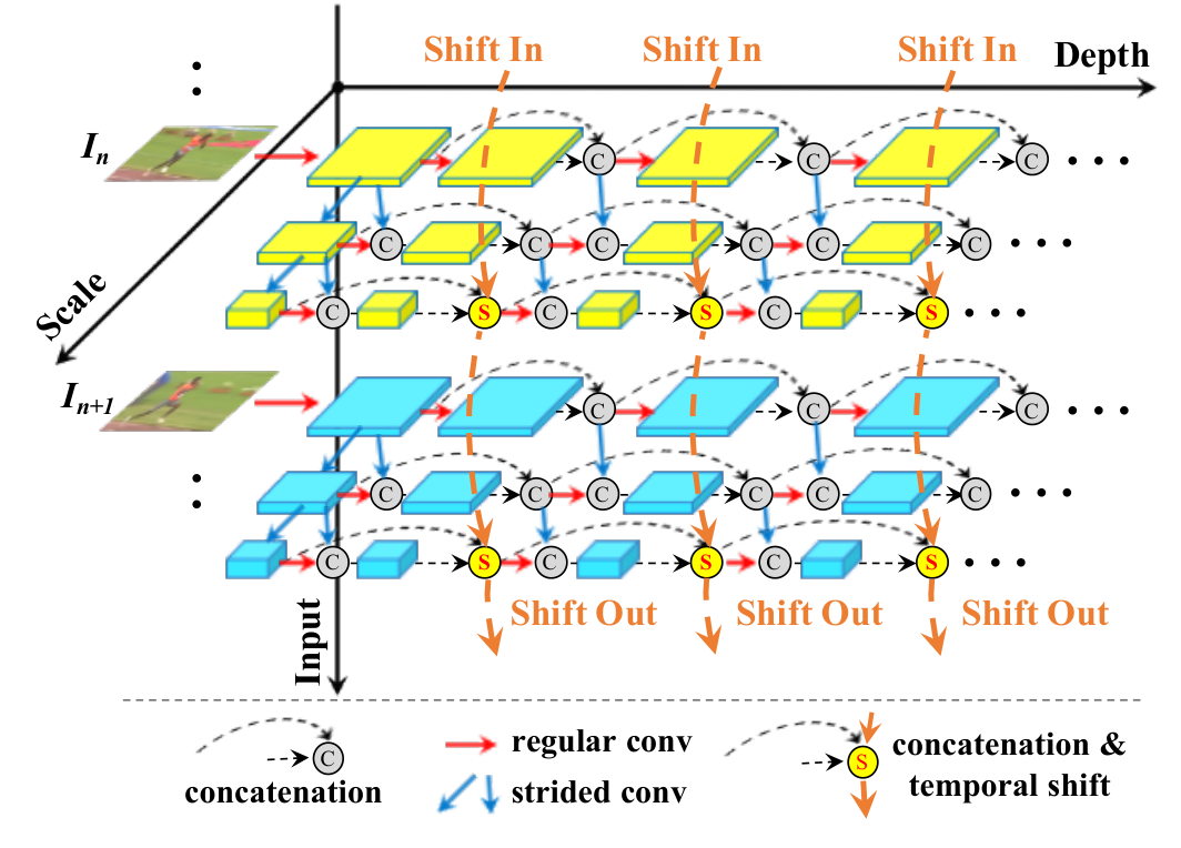
To tackle the problem of missing temporal relation when only 2D convolutions are applied on input frames, we adopt a temporal shift module for efficient temporal modeling. The original temporal shift module tsm shifts part of the channels from feature maps of each input frame forward and backward to that of its adjacent input frames, which facilitates information exchange among neighbouring frames with zero FLOPs cost and negligible time cost. Under dynamic inference circumstance, the original TSM cannot meet the requirement of progressive computation since the final feature maps have to rely on those of its later input frames. To integrate TSM into our framework, we tailor original TSM approach by only applying forward shift, which makes it possible for online process and it is called online temporal shift. Specifically, we add an online temporal shift module between and for arbitrary and to fully take advantage of multi-stride input brought by the frame permutation. The overall unified framework is shown in Fig.2(d). It is worthy of noting that, our method is a general design, when the checkpoints are located in the last row or last column, it is specialized to be input-wise or depth-wise dynamic inference framework.
4 Experiments
To validate effectiveness of our idea and provide comprehensive understanding on dynamic inference, we implemented three sample frameworks based on state-of-the-art 2D CNN MSDNet-38 msdnet, ResNet-50 and ResNet-101 resnet, respectively. More deeper and powerful backbones could be leveraged, but here we do not show such experiments because 1) we focus on efficient action recognition and heavy network is not suitable; 2) the three instances are able to achieve proof of concept purpose. MSDNet-38 contains five blocks (M=5) and four scales (S=4) are used in each block. Note that the online temporal shift module is only adopted on feature maps at the coarsest scale for all layers except the first layer. Fig. 3 illustrated the framework using only three scales for convenience. is 6 for MSDNet and each prediction head is composed of an average pooling and a linear layer. For ResNet, online temporal shift model is added at each residual block and we only append early-exit classifiers to the Res3, Res4 and Res5 and is set to 4 (the last 4 checkpoints in Fig. 2(d)). is determined as follows: the #FLOPs at the checkpoint is a known prior and is the total number of videos. We denote by a fixed exit probability that a sample that reaches a checkpoint will obtain a classification with sufficient confidence to exit. We assume that is constant across all checkpoints, which allows us to compute the probability that a sample exits at the checkpoint as: , where is a normalizing constant that ensures that . Given average inference budget in FLOPs, this gives rise to the constraint . We can solve this constraint for and determine the thresholds on a validation set in such a way that approximately validation samples exit at the checkpoint.
4.1 Datasets and Evaluation Metrics
To comprehensively evaluate our proposed method, we perform extensive experiments on the recent large scale dataset named Kinetics-400 kay2017kinetics. We also conduct experiments on heavy temporal relation sensitive datasets, including Something-Something v1 & v2 sth-sth. For these datasets, the actions therein mainly include object-object and human-object interactions, which require strong temporal relation to well categorizing them. Moreover, transfer learning experiments on the UCF-101ucf101 and HMDB-51hmdb, which are much smaller than Kinetics-400, is carried out to show the transfer capability of our solution. The evaluation metric is top-1 precision for Kinetics-400 and Something-Something. We also report average FLOPs/Video in the testing phase as well as the number of model parameters to depict model complexity. In this paper, we only use the RGB frames of these datasets for experiments.
4.2 Implementation Details
Training Data augmentation and preprocessing strategy is the same as TSN tsn. In our experiments, is set to 16. To evaluate the proposed network on several action recognition datasets, we pre-trained MSDNet-38, ResNet-50, ResNet-101 on the ImageNet-1k deng2009imagenet for initialization. The loss is the sum of cross-entropy at each checkpoint. For Kinetics-400, Something-Something v1 & v2, we start training with a learning rate of 0.01 and reduce it by a factor of 10 at 25, 35, 45 epochs and stop at 50 epochs. Dropout ratio is 0.5. Since UCF-101 and HMDB-51 are not large enough and are prone to over-fitting, we followed the common practice to use Kinetics pre-trained model as initialization and in total 25 epochs are trained, with an initial learning rate of 0.01 and it is decayed by 10x every ten epochs. Higher dropout ratio of 0.8 is used. Stochastic gradient descent (SGD) with a mini-batch size of 128 is utilized as an optimizer, and its momentum and weight decay value is set to 0.9 and 5e-4, respectively. BatchNorm layers bn are all finetuned during training.
Inference We apply single centre 224x224 cropping to predict the class labels and the 16 frames are evenly sampled from videos. To get the accuracy-FLOPs curves in the paper, we traverse different budget to determine on the train set and measure the actual accuracy and FLOPs. As for validation set, we use the critical point of , where accuracy drops little and FLOPs are smaller than full inference, obtained from the accuracy-FLOPs curve on the validation set to determine for testing and then accuracy and average #FLOPs per video is calculated.
4.3 Empirical Analysis
MSDNet v.s. ResNet First of all, we would like to know how backbone makes a difference. Both Kinetics-400 and Something-Something v2 is used to evaluate the dynamic inference mechanisms proposed in Section 3 using the RGB modality. As shown in Fig. 4(a), MSDNet-38 performs better than ResNet-50 in depth-wise dynamic inference owing to the multi-scale feature maps and dense connectivity. Influenced by the limited performance of depth-wise dynaimc inference, joint depth-wise and network depth-wise solution performed worse than input-wise dynamic inference for ResNet-50. On Something-Something v2, similar observations can be found.
Ablation studies Fig. 5 and Fig. 6 show the results based on MSDNet under different dynamic inference settings. Accordingly, the effectiveness of each component in our framework is analyzed as follows.
Depth-wise dynamic inference As shown in Fig. 5 and Fig. 6, it can be concluded from the results that depth-wise dynamic inference is effective on both datasets no matter whether the online temporal shift is enabled or not. It is a very interesting observation from the results of Fig. 6(b) that depth-wise dynamic inference with online temporal shift on Something-Something v2 performs even slightly better the joint input-wise and depth-wise adaptation. This is reasonable because temporal relation is crucial for this dataset, input adaptation brings very little gain such that network trained with pure depth-wise adaptation can be more competitive than its joint depth-wise and input-wise version. We can see that on Something-Something v2, without and with the online temporal shift, depth-wise adaptation achieves top-1 accuracy of 31.75% and 60.02%, and the #FLOPs can be reduced to 44.6G and 35.4G, respectively.
Input-wise dynamic inference and frame permutation We find that on Something-Something v2, input-wise adaptation brings negligible FLOPs saving, while on Kinetics-400 it can save FLOPs to some extent. In Fig. 5 and Fig. 6, on both datasets, it is clear that frame permutation improves input-wise adaptation, regardless of whether online temporal shift module is used or not. Even though temporal relation is not so crucial on Kinetics-400 compared to Something-Something v2, frame permutation still gains a lot, and we can infer that temporal coverage of the input sequence is essential to video classification. Naturally, other architectures such as TSM, can also benefit from the frame permutation mechanism for dynamic inference.
Online temporal shift Temporal modeling by online temporal shift is also essential for the final performance. It is seen from the figures, the online temporal shift improves the top-1 accuracy upper bound of our framework from 69.32% to 71.17% and 31.64% to 59.80% on Kinetics-400 in Fig. 5 and Something-Something v2 in Fig. 6, respectively.
Joint input-wise and depth-wise dynamic inference On Kinetics, the proposed joint solution benefits from an adaption of both dimensions in Fig. 5. The #FLOPs is reduced to 24.3G and 26.5G from 52G without or with the online temporal shift, respectively. We also show the distribution of videos predicted at each checkpoint in Table.2. However, in Fig. 6, on Something-Something v2, it performs comparably with or even slightly worse than depth-wise adaption owing to the heavy temporal dependency characteristic of the dataset and input-wise adaptation can hardly bring any gain.
Framework Backbone Input # Clips Prec@1 # Params FLOPs/Video I3D i3d 3D BN-Inception [All3256256]1 71.1 12.7M 544.44G S3D s3d 3D BN-Inception [All3224224]1 72.20 8.8M 518.6G ARTNet with TSN ARN 3D ResNet-18 [163112112]250 69.2 35.2M 5925G MF-Net mfnet - [163224224]1 65.00 8.0M 11.1G [163224224]50 72.80 555G ECO eco BN-Inception+3D ResNet-18 [163224224]1 69.00 47.5M 64G R(2+1)D RGB r2+1d ResNet-34 [323112112]10 72.00 63.8M 1524G Nonlocal-I3d nonlocal ResNet-50 [1283224224]1 67.30 35.33M 145.7G [1283224224]30 76.50 4371G TSN RGB tsn BN-Inception [253112112]10 69.1 10.7M 500G ResNet-50 [83224224]1 66.80 24.3M 33G ResNet-50 [163224224]1 67.80 24.3M 64G TSM lin2018tsm ResNet-50 [83224224]1 70.60 24.3M 33G [163224224]1 72.50 24.3M 64G StNet stnet ResNet-50 [2515256256]1 69.85 33.16M 189.29G ResNet-101 [2515256256]1 71.38 52.15M 310.50G Proposed MSDNet-38 (Full) [163224224]1 71.17 62.31M 52G MSDNet-38 [163224224]1 71.20 62.31M 26.5G ResNet-50 [163224224]1 72.57 29.12M 35G ResNet-101 [163224224]1 74.70 48.12M 66G
4.4 Comparison with State-of-the-arts
Results on Kinetics-400 We evaluate the proposed framework against the recent state-of-the-art 2D/3D convolution-based solutions. Extensive experiments are conducted on the Kinetics-400 to compare all models in terms of their effectiveness (i.e., top-1 accuracy) and efficiency (reflected by the total number of model parameters and FLOPs needed in the inference phase). Results are summarized in Table 1. To be noted, the latest camera ready version of TSM reported results of these datasets using dense sampling for higher performance. Hence, in this paper we cited the results of these datasets using uniform sampling reported in its arXiv v1 version lin2018tsm.
The results show that our proposed dynamic inference with MSDNet-38 backbone achieves top-1 precision of 71.20% with single RGB modality, and it requires only 26.5G FLOPs per video on average. When large backbone models are used, our method still strike good performance-FLOPs trade-off. Compared to StNet-Res101, our method with ResNet-50 exhibits better recognition performance (72.57% v.s. 71.38%), but the #FLOPs are significantly reduced by over (from 310G to 35G). When compared to the recent state-of-the-art ECO and TSM-Res50, our model improves the accuracy from 69% and 72.5% to 72.57%, meanwhile the #FLOPs is reduced from 64G and 64G to 35G, respectively. Other methods, such as MF-Net, S3D, and R(2+1)D, though their marginal performance gains are obtained at the price of at least 10 times of computation cost, our method with ResNet-101 still achieve better recognition performance than them while #FLOPs is only 66G. In brief, our model achieves excellent performance-cost trade-off with different backbones.
Checkpoint 1 2 3 4 5 6 Total #Videos 1993 2392 2871 3445 4134 4961 19796
Method Backbone Pretrain FLOPs/Video Something-Something v1 Something-Something v2 top-1 val top-5 val top-1 val top-5 val top-1 test top-5 test ECO16F BNInception+ Kinetics 64G 41.4 - - - - - ECO 3D ResNet-18 267G 46.4 - - - - - I3D 3D ResNet-50 Kinetics 306G 41.6 72.2 - - - - Non-local I3D+GCN 606G 46.1 76.8 - - - - TSN8F ResNet-50 Kinetics 33G 19.7 46.6 27.8 57.6 - - TSN16F 65G 19.9 47.3 30.0 60.5 - - TRN Multiscale BNInception ImageNet 33G 34.4 - 48.8 77.6 50.9 79.3 TRN Two-Stream - 42.0 - 55.5 83.1 56.2 83.2 TSM8F ResNet-50 Kinetics 33G 43.4 73.2 58.2 84.8 - - TSM16F 65G 44.8 74.5 58.7 84.8 59.9 85.9 Proposed ResNet-50 ImageNet 52.8(v1)/48.0G(v2) 45.2 75.2 58.2 85.2 - - MSDNet-38 38.4G(v1)/35.4G(v2) 46.5 75.6 60.0 86.2 60.1 86.6
Results on Something-Something v1 & v2 The Something-Something datasets are more complicated than Kinetics, the comparison of our solution against existing state-of-the-arts are list in Table 3. It is observed that, with 16 frames as input, our solution achieves state-of-the-art top-1 accuracy of 46.5% on Something-Something v1 validation set and 60.02% on v2. The #FLOPs of our model is 38.4G/35.4G on v1 and v2 respectively, which is much smaller than ECO, Non-local I3D+GCN and TSM16F. Compared to TSM on both datasets, our method achieves better recognition performance than TSM16F while the #FLOPs is comparable with TSM8F. We have also submitted the testing results of Something-Something v2 and results show that the testing performance of our solution is as high as in terms of top-1 accuracy.
4.5 Transfer Learning on UCF-101 & HMDB-51
Method Backbone FLOPs UCF-101 HMDB-51 ARTNet with TSN 3D ResNet-18 5925G 94.3 70.9 ECO BNInception+ 64G 92.8 68.5 3D ResNet-18 I3D RGB 3D Inception-v1 544G 95.1 74.3 TSN RGB BNInception 500G 91.1 - TSN8F ResNet-50 33G 91.5 63.2 TSN16F 64G 91.4 63.6 TSM8F ResNet-50 33G 94.0 70.3 TSM16F 64G 94.5 70.7 StNet ResNet-50 53G 93.5 - Proposed MSDNet-38 15.8G 94.2 - 29.2G - 70.1 ResNet-50 18.5G 94.7 - 34.4G - 72.34 ResNet-101 34.6G 95.3 - 69.1G - 73.48
We transfer the proposed models pre-trained on Kinetics-400 to the much smaller datasets of UCF-101 and HMDB-51 to show that our method can be well generalized to other datasets. Fig. 7 show the Mean Class Accuracy v.s. Average FLOPs/Video curve on the split1 of UCF-101 and HMDB-51, respectively. For UCF-101 split1, the average FLOPs can be reduced by 70% while remaining the same performance with full inference. It is also be observed with 1% accuracy degradation, around 80% reduction in average FLOPs is achieved. For HMDB-51, our dynamic inference scheme keep classification accuracy while reducing up to 45% average FLOPs. Besides, the accuracy on UCF-101 is much higher than HMDB-51, and we believe that our method can reduce more average FLOPs on easier dataset. We also observe that the curve of HMDB-51 is similar to that of Kinetics-400 because the accuracy of our model is very close on these two scene-based datasets.
When compared with other methods, our model is evaluated by following the common practice of averaging accuracy/FLOPs over three training/testing splits of both datasets. The evaluation results can be found in Table 4. From this table, we can see that our model shows a pretty transfer capability. It obtains pretty good accuracy on UCF-101 and HMDB-51, and the mean class accuracy is 94.2% and 70.1%, respectively, which is comparable to or even better than performances of many state-of-the-art solutions. Besides, our model achieves great efficiency improvement, and the average FLOPs/Video can be significantly reduced to 15.8G and 29.2G on UCF-101 and HMDB-51. The results of ResNet based models can be analyzed similarly.
5 Discussion
Parallelism Dynamic inference, compared with fixed inference, could degrade the parallelism capability to some extent, but it can be paralleled. The depth-wise dynamic inference can be paralleled in the input dimension, meanwhile input-wise dynamic inference can be paralleled in the input dimension when the computation process is going from one checkpoint to the next one and more than one frames are fed. As for the joint input-wise and depth-wise scheme, it’s parallelism capability is further limited, take Fig.2(d) for illustration, if the computation process goes from the checkpoint to the one, the last block outputs of can be calculated in parallel. When it travels from the checkpoint to the last one, the whole feature extraction process of can be paralleled.
Optimality In this paper, our key insight is dynamic inference and we formally summarize its general idea and provide sample instantiating strategies to prove its feasibility. The three framework instances are designed to thoroughly analyze effectiveness of our idea. However, the optimality of these frameworks are not necessarily guaranteed. For example, how these thresholds can be adaptively determined for different videos at different checkpoints; how the checkpoints can be dynamically located from video to video and so on. We believe that all of these problems deserve future research effort.
6 Conclusion
In this paper, we focus on improving action recognition efficiency in videos by dynamic inference, which takes advantage of distinguishability variation among different videos. Both the proposed frame permutation and online temporal shift scheme contribute largely to performance improvement. By exploiting dynamic inference, our models are verified on multiple well-known datasets being able to significantly save average FLOPs consumption per video while remaining recognition performance unaffected. To our best knowledge, we are the first to propose dynamic inference for efficient video recognition, and it is proven to be a promising direction.
References
- (1) Joao Carreira and Andrew Zisserman. Quo vadis, action recognition? a new model and the kinetics dataset. In CVPR, 2017.
- (2) Yunpeng Chen, Yannis Kalantidis, Jianshu Li, Shuicheng Yan, and Jiashi Feng. Multi-fiber networks for video recognition. In ECCV, 2018.
- (3) Jia Deng, Wei Dong, Richard Socher, Li-Jia Li, Kai Li, and Li Fei-Fei. Imagenet: A large-scale hierarchical image database. In CVPR, 2009.
- (4) Ali Diba, Vivek Sharma, and Luc Van Gool. Deep temporal linear encoding networks. In CVPR, 2017.
- (5) Christoph Feichtenhofer, Axel Pinz, and Richard Wildes. Spatiotemporal residual networks for video action recognition. In NIPS, 2016.
- (6) Christoph Feichtenhofer, Axel Pinz, and Richard P Wildes. Temporal residual networks for dynamic scene recognition. In CVPR, 2017.
- (7) Michael Figurnov, Maxwell D Collins, Yukun Zhu, Li Zhang, Jonathan Huang, Dmitry Vetrov, and Ruslan Salakhutdinov. Spatially adaptive computation time for residual networks. In CVPR, 2017.
- (8) Rohit Girdhar, Deva Ramanan, Abhinav Gupta, Josef Sivic, and Bryan Russell. Actionvlad: Learning spatio-temporal aggregation for action classification. In CVPR, 2017.
- (9) Raghav Goyal, Samira Ebrahimi Kahou, Vincent Michalski, Joanna Materzynska, Susanne Westphal, Heuna Kim, Valentin Haenel, Ingo Fruend, Peter Yianilos, Moritz Mueller-Freitag, et al. The” something something” video database for learning and evaluating visual common sense. In ICCV, 2017.
- (10) Jian Guo and Stephen Gould. Depth dropout: efficient training of residual convolutional neural networks. In 2016 International Conference on Digital Image Computing: Techniques and Applications (DICTA). IEEE, 2016.
- (11) Dongliang He, Zhichao Zhou, Chuang Gan, Fu Li, Xiao Liu, Yandong Li, Limin Wang, and Shilei Wen. Stnet: Local and global spatial-temporal modeling for action recognition. In AAAI, 2019.
- (12) Kaiming He, Xiangyu Zhang, Shaoqing Ren, and Jian Sun. Deep residual learning for image recognition. In Proceedings of the IEEE conference on computer vision and pattern recognition, pages 770–778, 2016.
- (13) Gao Huang and Danlu Chen. Multi-scale dense networks for resource efficient image classification. ICLR, 2018.
- (14) Gao Huang, Yu Sun, Zhuang Liu, Daniel Sedra, and Kilian Q Weinberger. Deep networks with stochastic depth. In ECCV, pages 646–661. Springer, 2016.
- (15) Sergey Ioffe and Christian Szegedy. Batch normalization: Accelerating deep network training by reducing internal covariate shift. In ICML, 2015.
- (16) Will Kay, Joao Carreira, Karen Simonyan, Brian Zhang, Chloe Hillier, Sudheendra Vijayanarasimhan, Fabio Viola, Tim Green, Trevor Back, Paul Natsev, et al. The kinetics human action video dataset. arXiv preprint arXiv:1705.06950, 2017.
- (17) Hildegard Kuehne, Hueihan Jhuang, Estíbaliz Garrote, Tomaso Poggio, and Thomas Serre. Hmdb: a large video database for human motion recognition. In ICCV. IEEE, 2011.
- (18) Myunggi Lee, Seungeui Lee, Sungjoon Son, Gyutae Park, and Nojun Kwak. Motion feature network: Fixed motion filter for action recognition. In ECCV, 2018.
- (19) Ji Lin, Chuang Gan, and Song Han. Tsm: Temporal shift module for efficient video understanding. arXiv preprint arXiv:1811.08383v1, 2018.
- (20) Ji Lin, Chuang Gan, and Song Han. Tsm: Temporal shift module for efficient video understanding. In Proceedings of the IEEE International Conference on Computer Vision, 2019.
- (21) Xiang Long, Chuang Gan, Gerard de Melo, Jiajun Wu, Xiao Liu, and Shilei Wen. Attention clusters: Purely attention based local feature integration for video classification. In CVPR, 2018.
- (22) Zhaofan Qiu, Ting Yao, and Tao Mei. Learning spatio-temporal representation with pseudo-3d residual networks. In ICCV, 2017.
- (23) Karen Simonyan and Andrew Zisserman. Two-stream convolutional networks for action recognition in videos. In NIPS, 2014.
- (24) Khurram Soomro, Amir Roshan Zamir, and Mubarak Shah. Ucf101: A dataset of 101 human actions classes from videos in the wild. arXiv preprint arXiv:1212.0402, 2012.
- (25) Shuyang Sun, Zhanghui Kuang, Lu Sheng, Wanli Ouyang, and Wei Zhang. Optical flow guided feature: A fast and robust motion representation for video action recognition. In CVPR, 2018.
- (26) Du Tran, Lubomir Bourdev, Rob Fergus, Lorenzo Torresani, and Manohar Paluri. Learning spatiotemporal features with 3d convolutional networks. In ICCV, 2015.
- (27) Du Tran, Heng Wang, Lorenzo Torresani, Jamie Ray, Yann LeCun, and Manohar Paluri. A closer look at spatiotemporal convolutions for action recognition. In CVPR, 2018.
- (28) Limin Wang, Wei Li, Wen Li, and Luc Van Gool. Appearance-and-relation networks for video classification. In CVPR, 2018.
- (29) Limin Wang, Yuanjun Xiong, Dahua Lin, and Luc Van Gool. Untrimmednets for weakly supervised action recognition and detection. In CVPR, 2017.
- (30) Limin Wang, Yuanjun Xiong, Zhe Wang, Yu Qiao, Dahua Lin, Xiaoou Tang, and Luc Van Gool. Temporal segment networks: Towards good practices for deep action recognition. In ECCV. Springer, 2016.
- (31) Xiaolong Wang, Ross Girshick, Abhinav Gupta, and Kaiming He. Non-local neural networks. In CVPR, 2018.
- (32) Wenhao Wu, Dongliang He, Xiao Tan, Shifeng Chen, and Shilei Wen. Multi-agent reinforcement learning based frame sampling for effective untrimmed video recognition. In Proceedings of the IEEE International Conference on Computer Vision, pages 6222–6231, 2019.
- (33) Saining Xie, Chen Sun, Jonathan Huang, Zhuowen Tu, and Kevin Murphy. Rethinking spatiotemporal feature learning: Speed-accuracy trade-offs in video classification. In ECCV, 2018.
- (34) Mohammadreza Zolfaghari, Kamaljeet Singh, and Thomas Brox. Eco: Efficient convolutional network for online video understanding. In ECCV, 2018.