-Regularized High-dimensional Accelerated Failure Time
Model
Xingdong Feng
Jian Huang
Yuling Jiao
Shuang Zhang
Note: Xingdong Feng is
Professor and Shuang Zhang is PhD candidate, School of Statistics and Management, Shanghai University of Finance and Economics, Shanghai 200433, China (email: feng.xingdong@mail.shufe.edu.cn). Jian Huang is Professor, Department of Statistics and Actuarial Science, University of Iowa, Iowa City, Iowa 52246, USA (email: jian-huang@uiowa.edu). Yuling Jiao is Associate Professor, School of Mathematics and Statistics, Wuhan University, Wuhan 430000, China (email: yulingjiaomath@whu.edu.cn). This work was supported by NSF grant DMS-1916199, National Natural Science Foundation of China (No. 11971292, No. 11690012 and No.11871474), and Program for Innovative Research Team of SUFE.
August 11, 2026
Abstract
We develop a constructive approach for -penalized estimation in the sparse accelerated failure time (AFT)
model with high-dimensional covariates.
Our proposed method is based on Stute’s weighted least squares criterion combined with -penalization.
This method is a computational algorithm that generates a sequence of solutions iteratively, based on active sets derived from primal and dual information and root finding according to the KKT conditions.
We refer to the proposed method as AFT-SDAR (for support detection and root finding).
An important aspect of our theoretical results is that we directly concern the sequence of solutions generated based on the AFT-SDAR algorithm. We prove that the estimation errors of the solution sequence decay exponentially to the optimal error bound
with high probability, as long as the covariate matrix satisfies a mild regularity condition which is necessary and sufficient for model identification even in the setting of high-dimensional linear regression.
We also proposed an adaptive version of AFT-SDAR, or AFT-ASDAR, which determines the support size of the estimated
coefficient in a data-driven fashion.
We conduct simulation studies to demonstrate the superior performance of the proposed method over the lasso and MCP in terms of accuracy and speed.
We also apply the proposed method to a real data set to illustrate its application.
Key Words: Censored data; -penalization; KKT condition; primal and dual information; support detection
1 Introduction
In survival analysis, an attractive alternative to the widely used proportional hazards model
(Cox 1972)
is the accelerated failure time (AFT) model
(Koul et al. 1981; Wei 1992; Kalbfleisch and Prentice 2011).
The AFT model is a linear regression model in which the response variable is usually the logarithm or a known monotone transformation of the failure time.
Let be the failure time and be a -dimensional covariate vector for the th subject in a random sample of size . The AFT model assumes
where is the underlying regression coefficient vector, ’s are random error terms.
When is subject to right censoring, we only observe , where , is the censoring time, and is the censoring indicator.
Assume that a random sample of i.i.d. observations (, , ), , is
available.
To estimate when the distribution of the error terms is unspecified, several approaches have been proposed in the literature.
One approach is the Buckley-James estimator
(Buckley and James 1979),
which adjusts for censored observations using the Kaplan-Meier
estimator. The second approach is the rank-based estimator
(Ying 1993),
which is motivated by the score function of the partial likelihood.
Another interesting alternative is the weighted least squares approach
(Stute et al. 1993; Stute 1996),
which involves the minimization of a weighted least squares objective function.
In this paper, we focus on the high-dimensional AFT model, where the dimension of the covariate vector can exceed the sample size.
In the high-dimensional AFT model,
many researchers have proposed methods for parameter estimation and variable selection.
For example,
Huang et al. 2006
considered the LASSO
(Tibshirani 1996)
in the AFT model, based on the weighted least squares criterion;
Johnson 2008 and Johnson et al. 2008
applied the SCAD
(Fan and Li 2001)
penalty to the rank-based estimator and Buckley-James estimator;
Cai et al. 2009
proposed the rank-based adaptive LASSO
(Zou 2006)
method;
Huang and Ma 2010
used the bridge penalization for the regularized estimation and variable selection;
Hu and Chai 2013
extended the MCP
(Zhang et al. 2010)
penalty to the weighted least square estimation;
Khan and Shaw 2016
used the adaptive and weighted elastic net methods
(Zou and Zhang 2009; Hong and Zhang 2010)
based on the weighted least squares criterion.
We propose an -penalized method for estimation and variable selection in the high-dimensional AFT model. We extend the support detection and root finding (SDAR) algorithm
(Huang et al. 2018)
for linear regression model to the
AFT model. For convenience, we refer to the proposed method as AFT-SDAR.
In the same spirit as the SDAR method, AFT-SDAR is a constructive approach to estimating the sparse and high-dimensional AFT model. This approach is a computational algorithm motivated from the KKT conditions for the -penalized weighted least squares solution, and generates a sequence of solutions iteratively, based on support detection using primal and dual information and root finding.
Theoretically, we show that the -norm of the estimation errors of the solution sequence decay exponentially to the optima order with high probability, as long as the covariate matrix satisfies the weakest regularity condition that is necessary and sufficient for model identification. Moreover, the estimated support coincides with the true support of the underlying vector regression coefficients if the minimum absolute value of the nonzero entries of the target is above the detectable order.
The rest of this paper is organized as follows. In Section 2, we described the -penalized criterion for the AFT model.
In Section 3, we give the KKT conditions for the -penalized weighted least squares solutions and describe the proposed AFT-SDAR algorithm.
In Section 4, we first establish the finite-step and deterministic
error bounds for
the solution sequence generated by the AFT-SDAR algorithm.
As a consequence of these deterministic error bounds, we provide nonasymptotic error bounds for the solution sequence.
We also show that the proposed method recovers the support of the underlying regression coefficient vector in finite iterations with high probability.
In Section 5, we describe
AFT-ASDAR, the adaptive version of AFT-SDAR that selects the tuning parameter in a data driven fashion. In Section 6, we assess the finite sample performance of the proposed method with different simulation studies and a real case study on a breast cancer gene expression data set.
Concluding remarks are given in Section 7. Proofs for all the lemmas and theorems are deferred to Appendix. An R package implementing the proposed method is available at https://github.com/Shuang-Zhang/ASDAR/.
2 AFT regression with -penalization
Let be the order statistics of ’s. Let be the associated censoring indicators and let be the associated covariates.
In the weighted least squares method,
the weights ’s are the jumps in Kaplan-Meier estimator based on
, , which can be expressed as
(1)
The weighted least squares criterion is given by
In the low-dimensional settings with , this criterion leads to a consistent and asymptotically normal estimator under appropriate conditions (Stute et al. 1993; Stute 1996).
However, in the high-dimensional settings when , regularization is needed to ensure a unique solution in
minimizing .
We consider the -regularized method for variable selection and estimation in AFT based on the weighted least squares criterion.
The -penalized estimator is given by
(2)
where is a tuning parameter, and denotes the number of nonzero elements of .
To facilitate computation, we rewrite the weighted least squares loss as a standard least squares loss as follows. Let the design matrix be and let . Define
Without loss of generality, assume that , , hold throughout this paper, where is the th column of . Let
Define
and .
Then each column of is -length and supp()=supp(), where supp()=.
Let
Define
(3)
Then the estimator of defined in (2) can be obtained as
3 AFT-SDAR Algorithm
We first introduce some notation used throughout the paper.
Let be the usual () norm
of the vector .
Let denote the cardinality of the set . Denote , with its th element , where is the indicator function. Let
and
be the th largest elements (in absolute value) and the minimum absolute value of , respectively. Let denote the maximum value (in absolute value) of the matrix . Let denote the gradient of
function . Denote , where is a column of a matrix . Let be the minimum eigenvalue of the matrix and be the spectrum norm of the matrix .
Denote
.
The following lemma gives the KKT conditions of the minimizer of (3).
Conversely, if and satisfy (4), then is a local minimizer of (3), and
is a local minimizer of (2).
Our proposed AFT-SDAR algorithm is based on solving the KKT equations
(4) iteratively.
Let and .
Based on (4) and by the definition of , we have
and
(6)
We solve these equations iteratively.
Let be the values at the th iteration,
and let be the active and inactive sets based on
, where
(7)
Then based on (6), we calculate the updated values
as follows:
(8)
Suppose that for some ,
where .
At the th iteration, we set
(9)
in (7). Hence in every iteration due to this . Note that the tuning parameter is expressed in terms of . We will use a data-driven procedure to tune the cardinality in Section 5.
Let be an initial value, then we get a sequence of solutions by using (7)
and (8) with the value of given in (9).
We introduce a step size
in the definitions of the active and inactive sets as follows:
(10)
with .
The step size plays the role of weighing the importance of and in determining the active and inactive sets.
In order to bound the estimation error of the sequences generated by AFT-SDAR, we need some regularity conditions on the covariate matrix. Thanks to
this step size , we can replace the sparse Riesz condition used in Huang et al. 2018
in analyzing the SDAR to the weakest condition possible, which is necessary and sufficient for model identification even in high-dimensional linear regression, see Section 4 for detail.
We describe the AFT-SDAR algorithm in detail in Algorithm 1.
Algorithm 1 AFT-SDAR
1:
Input: , , , T;
2:fordo
3:
, .
4:
.
5:
.
6:
.
7:
.
8:
.
9:
, then
10:
Stop and denote the last iteration , , , , .
11:else
12:
13:end if
14:endfor
15:
Output: and as the estimates of and respectively.
In Algorithm 1, we terminate the computation when for some , because the solution sequence generated by AFT-SDAR will not change afterwards. In Section 4, we provide sufficient conditions under which
with high probability, where ,
that is, the support of the underlying regression coefficient can be recovered in finite many steps.
4 Theoretical Properties
In this section, we consider the finite-step error bound for the solution sequence computed based on Algorithm 1.
We also study the probabilistic and nonasymptotic error bound
for the solution sequence.
We first consider the deterministic error bounds for the solution sequence generated
based on AFT-SDAR.
We choose the step size satisfies
(11)
with , and let be a constant satisfying
(12)
Theorem 1.
Suppose and set in Algorithm 1.
Suppose (11) and (12) hold.
For the solution at the th iteration in Algorithm 1, we have
(13)
(14)
where
We observe that the error bound consists of two terms as indicated in Theorem 1. For any given values
of observations, the first term converges to
zero exponentially. The magnitude of the second term is determined by
in
(13)
and
in (14),
which are given by the gradient of the weighted least squares criterion at the underlying parameter value. Therefore, under the model assumption, their expected values are zero and should be concentrated in a small neighborhood of zero.
To study the probabilistic and nonasymptotic error bounds of the solution sequences and , we make the following assumptions.
(C1)
There exists a constant such that .
(C2)
The error terms are independent and identically distributed with mean zero and finite variance . Furthermore, they are subgaussian, in the sense that there exist some constants such that for all and all .
(C3)
The covariates are bounded, that is, there exists a constant such that
(C4)
The error terms are independent of the Kaplan-Meier weights .
(C5)
There exists some positive constants and such that
, where
Remark 1.
Condition
(C1)
constrains the maximum absolute value of the matrix .
Condition (C2) on the subgaussion tails of the error terms is standard in high-dimensional regression models. Condition (C3) is assumed for technical convenience. It can be relaxed to with high probability.
Moreover, conditions (C2)-(C4) are assumed to ensure that
is small.
Condition
(C5) assumes that the signal is not too small, which
is needed for the target signal to be detectable.
Theorem 2.
Suppose and set in Algorithm 1.
Suppose (11) and (12) hold.
If
(C1)-(C5)
hold,
then with probability at least
,
Therefore,
with high probability if
To derive the sharp estimation error bound in Theorem 2, we need . This is guaranteed
by choosing stratifying (11) and satisfying (12), which only requires . This is a weakest possible condition even in high-dimensional linear regression model , where, , since is equivalent to the condition that the linear model is identifiable.
To be precise, let and If we wish to derive from , i.e., from , we need , which is
a sufficient and necessary condition.
However, in the analysis of SDAR algorithm
(Huang et al. 2018),
the authors assumed stronger conditions, i.e., sparse Riesz condition (SRC)
(Zhang and Huang 2008)
to obtain the estimation error bound. The condition is also weaker than the kinds of restricted strong convexity conditions used in
bounding the estimation error for the global solutions in penalized convex and nonconvex regressions, see Zhang and Zhang 2012, Wainwright 2019 and the references therein.
This result gives nonasymptotic error bound of the solution sequence.
In particular, when , the solution sequence converges
to the underlying regression coefficient with high probability.
The following theorem establishes the support recovery property of
AFT-SDAR.
Theorem 3.
Suppose and set in Algorithm 1.
Suppose (11) and (12) hold.
If (C1)-(C5)
hold,
then with probability at least
,
if , where is the ratio of the largest absolute coefficient over the smallest absolute nonzero coefficient of .
Theorem 3 demonstrates that the estimated support via AFT-SDAR will contain the true support with the cost at most number of iterations if the minimum signal strength of is above the detectable threshold .
Further, if we set in AFT-SDAR, then the stopping condition will hold if since the estimated supports coincide with the true support then.
As a consequence, the Oracle estimator will be recovered in steps.
Finally, we note that an important aspect of the results above is that they directly concern the sequence of solutions generated based on Algorithm 1, rather than a theoretically defined global solution to the nonconvex -penalized weighted least squares criterion. Thus there is no gap between our theoretical results and computational algorithm.
5 Adaptive AFT-SDAR
In practice, the sparsity level of the true parameter value or is unknown. Therefore, we can regard as a tuning parameter.
Let increase from 0 to , which is a given large enough integer. In general, we set as suggested by
Fan and Lv 2008,
where is a positive constant.
Then we can obtain a set of solutions paths: , where . Finally, we use the cross-validation method or HBIC criteria
(Wang et al. 2013)
to determine , the value of . Thus we can take with as the estimate of .
We can also run Algorithm 1 until by increasing , where is a given tolerance level. Then can be taken as the estimation of .
Furthermore, we can gradually increase to run Algorithm 1 until the residual sum of squares is less than a given tolerate level , then output at this time to terminate the calculation. In summary, we get an adaptive AFT-SDAR algorithm as described in Algorithm 2.
Algorithm 2 AFT-ASDAR
1:
Input: , , , an integer , an integer Q, an early stopping criterion (optional). Set .
2:fordo
3:
Run Algorithm 1 with and with initial value , . Denote the output by , .
4:if the early stopping criterion is satisfied or ,
then
5:
stop
6:else
7:
8:end if
9:endfor
10:
Output: and as the estimates of and respectively.
6 Numerical studies
In this section, we conduct simulation studies and real data analysis
to illustrate the effectiveness of the proposed method. We compare the simulation results of AFT-SDAR/AFT-ASDAR with those of Lasso and MCP in terms of accuracy and efficiency.
We also evaluate the performance
in terms of the effect of the model parameters including the sample size , the variable dimension , the correlation measure among covariates and the censoring rate .
Moreover, we examine the average number of iterations for AFT-SDAR
to converge.
We also apply AFT-SDAR to a real data set to illustrate its application.
We implemented Lasso and MCP for the AFT model
using the coordinate descent algorithm (Breheny and Huang 2011).
6.1 Accuracy and efficiency
We generate a random Gaussian matrix
whose entries are i.i.d. . Then the design matrix is generated with , , and , . Here is a measure of the correlation among covariates. The underlying regression coefficient vector with
nonzero coefficients is generated
such that the nonzero coefficients in are uniformly
distributed in , where
and .
The nonzero coefficients are randomly assigned to the components of .
For each subject,
the responses , where is generated independently from ,
and the censoring variable is generated independently from the uniform distribution , where controls the censoring rate such that the desired censoring rate can be obtained.
We compare AFT-SDAR, AFT-ASDAR with Lasso and MCP on the data generated from theses models.
In the implementation of AFT-ASDAR, we set , and terminate the computation if the residual is smaller than .
To examine the effect of the correlation measure ,
we set , , , , and , i.e., takes a grid of values from 0.3 to 0.9 with a step size 0.3.
Table 1: Numerical results (the averaged relative error, CPU time) on data sets with , , , , , .
Method
ReErr ()
Time(s)
0.3
Lasso
10.49
10.57
MCP
1.10
11.55
AFT-SDAR ()
0.51
4.44
AFT-ASDAR ()
0.52
4.60
AFT-SDAR ()
0.51
4.46
AFT-ASDAR ()
0.52
4.72
0.6
Lasso
11.07
12.95
MCP
2.10
10.91
AFT-SDAR ()
2.01
4.32
AFT-ASDAR ()
2.02
4.53
AFT-SDAR ()
1.93
4.62
AFT-ASDAR ()
1.93
4.89
0.9
Lasso
11.40
10.78
MCP
1.08
11.45
AFT-SDAR ()
0.65
4.42
AFT-ASDAR ()
0.65
4.63
AFT-SDAR ()
0.47
4.72
AFT-ASDAR ()
0.47
5.01
Table 1 shows the results
based on 100 independent replications of AFT-SDAR, AFT-ASDAR,
Lasso and MCP.
In Table 1, the first column gives the values of , the second column depicts the methods, the third column shows the averaged relative error (ReErr=), and
the fourth column shows the averaged CPU time.
It is clear from Table 1 that both AFT-SDAR and AFT-ASDAR tend to have smaller relative errors (ReErr) than those of Lasso and MCP.
When and 0.9, AFT-SDAR and AFT-ASDAR have smaller relative errors at than at .
In terms of the speed,
AFT-SDAR and AFT-ASDAR are more than twice as fast as Lasso and MCP for each and , respectively.
For a wide range of the correlation measure and the step size , AFT-SDAR and AFT-ASDAR perform well
in terms of relative error and computational speed. In addition, for
data with high correlations, choosing a step size less than the default value can lead to smaller relative errors.
6.2 Support recovery
We now assess the support recovery performance
of AFT-ASDAR, Lasso and MCP.
In AFT-ASDAR, we set the largest size of the support and the step size , and
use the HBIC criteria to chose the cardinality .
In the data generating models,
the rows of the design matrix are i.i.d. , where , .
Let , where and . The underlying regression coefficient vector is
generated in such a way that
the nonzero coefficients in are uniformly
distributed in ,
and is a randomly chosen subset of with .
The responses , where ’s are independently drawn from the normal distribution .
The censoring variable is generated independently from the uniform distribution as in Sect. 6.1.
All the simulation results reported below are based on 100 independent replications.
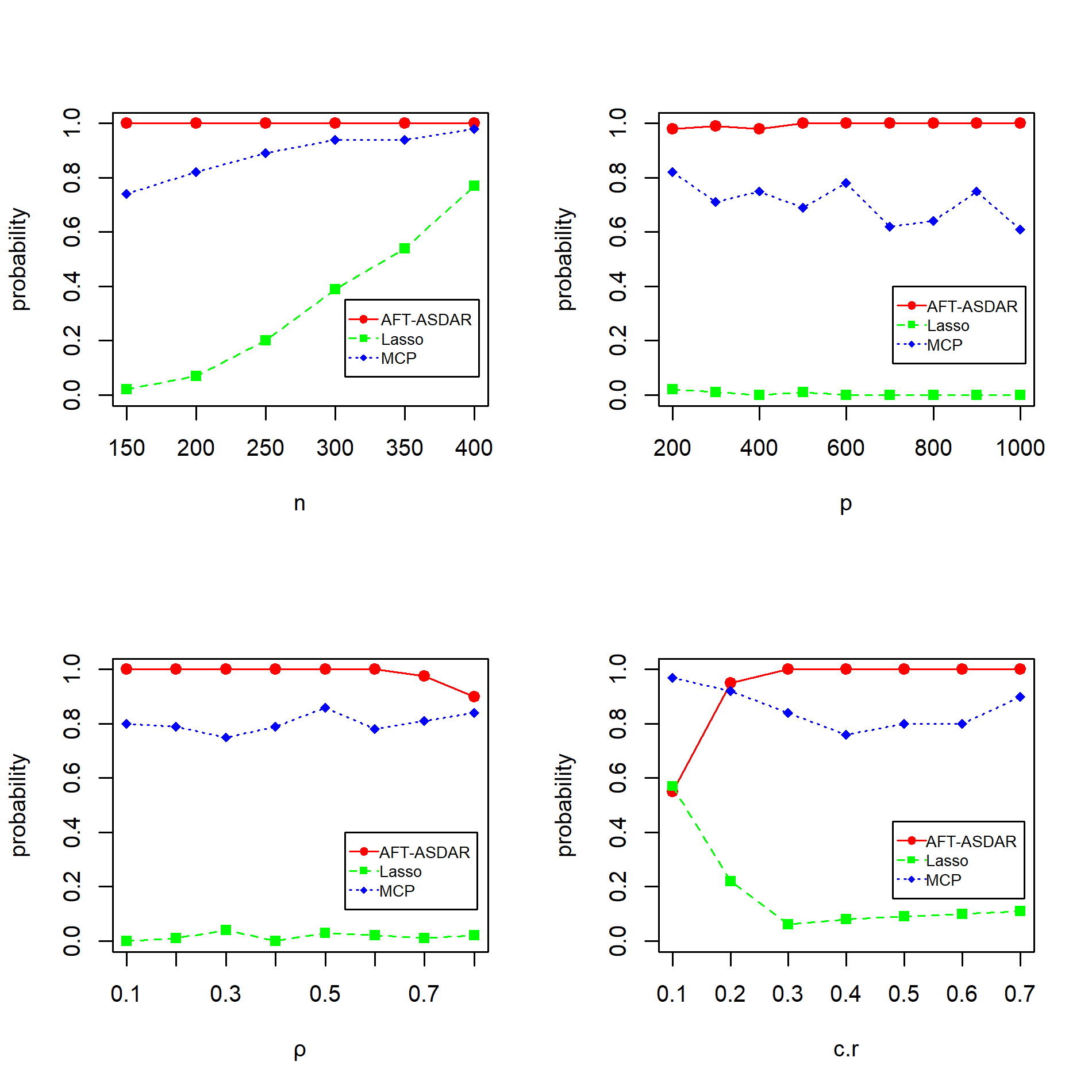
Figure 1: The numerical results of the influence of sample size (top left panel), variable dimension (top right panel), correlation (bottom left panel) and censoring rate (bottom right panel) on the probability of exact recovery of the true support sets
6.2.1 Influence of the sample size
We set , , , , , and in the data generating models.
The top left panel of Fig. 1 shows the influence of the sample size on the percentage of exact recovery of based
on 100 replications.
In these examples,
AFT-ASDAR tends to have the percentage of recovery close to 100%, while the percentage of Lasso is significantly less than 100%, and the percentage of MCP is less than 100% except when the sample size .
6.2.2 Influence of the variable dimension
We set , , , , , and in the models.
The top right panel of Fig. 1 shows the influence of the variable dimension on the percentage of exact recovery of .
The percentage of AFT-ASDAR is always close to 100% as the variable dimension increases, but those of both Lasso and MCP are always less than 100%. These results suggest that AFT-ASDAR performs better in selecting variables with an increasing variable dimension .
6.2.3 Influence of the correlation
We set , , , , , and . The bottom left panel of Fig. 1 shows the influence of the the correlation on the percentage of exact recovery of .
AFT-ASDAR has nearly 100% probability in support recovery except when .
When , the recovery percentage of
AFT-ASDAR is smaller than but still comparable with MCP.
6.2.4 Influence of the censoring rate
We set , , , , ,
and to generate the data.
The bottom right panel of Fig. 1 shows the influence of the censoring rate on the probability of exact recovery of .
As the censoring rate increases, the percentage of recovery of AFT-ASDAR is stable and remains close to 1, while the recovery percentages of Lasso and MCP are less than 1.
6.3 Number of iterations
To examine the convergence properties of
of AFT-SDAR, we conduct simulations to obtain the average number of iterations of AFT-SDAR with = in Algorithm 1.
We generate the data in the same way as described in
Section 6.2.
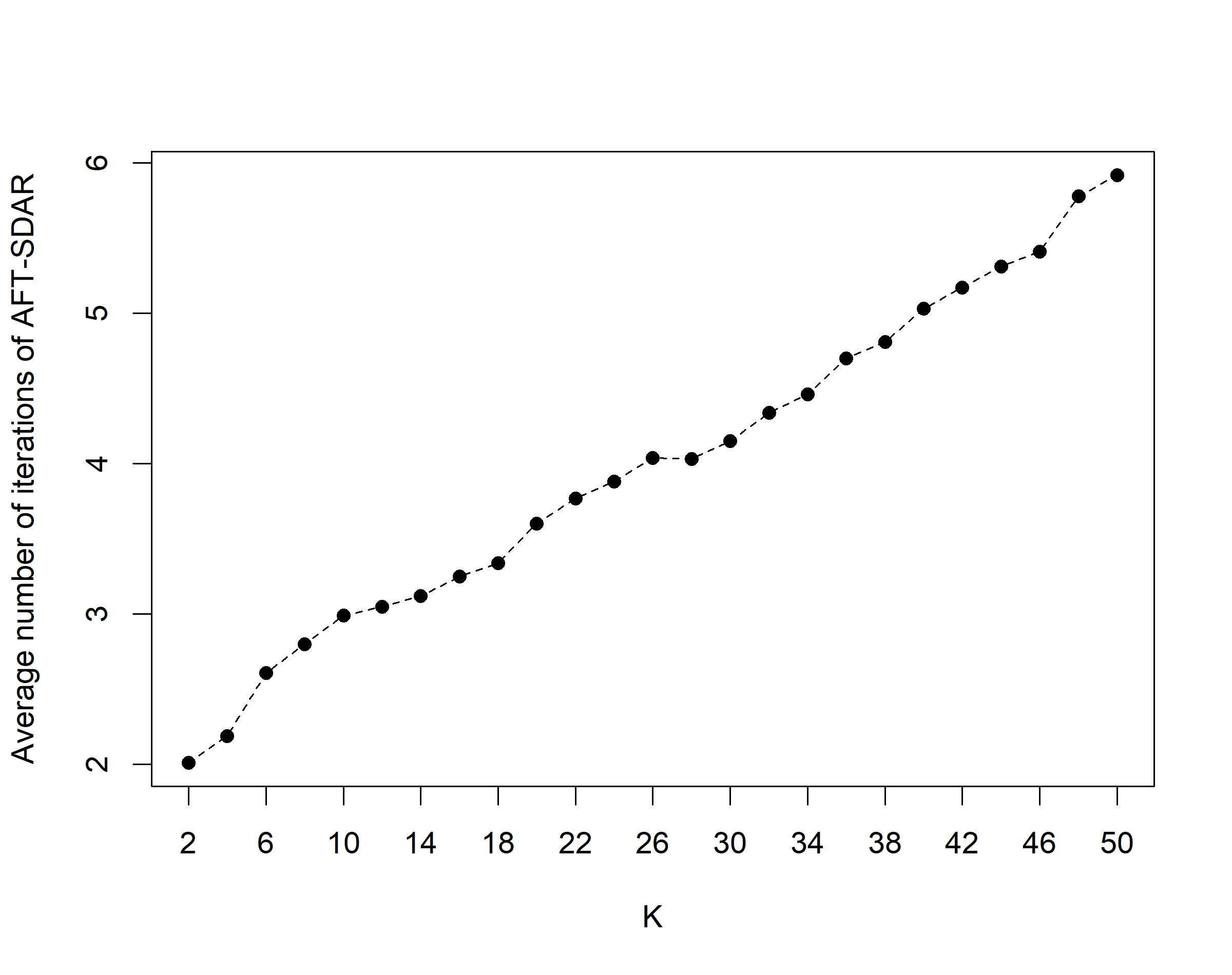
Figure 2 shows the average number of iterations of AFT-SDAR with
based on 100 independent replications on data set:
, , , , , , .
Figure 2: The average number of iterations of AFT-SDAR as K increases
As shown in Fig. 2, the average number of iterations of the AFT-SDAR algorithm increases as the number of important variables increases from 2 to 50. This is expected since it will take more iterations for the algorithm to converge when the model size increases.
However, even when , it only take six iterations for the algorithm to converge. This shows that AFT-SDAR has fast convergence in the simulation models considered here.
6.4 Real data exemple
In this section, we illustrate the proposed approach by analyzing the breast cancer data set nki70 from the study of
Van De Vijver et al. 2002.
The nki70 data set includes 144 lymph node positive breast cancer patients on metastasis-free survival, 5 clinical risk factors, and gene expression measurements of 70 genes found to be prognostic for metastasis-free survival in an earlier study, and the censoring rate is about .
We fit this data set with the AFT model. Further, we compare the estimation of the proposed approaches with that of Lasso and MCP. We set in AFT-SDAR, and implement AFT-ASDAR with .
Set in AFT-SDAR and AFT-ASDAR.
The results are showed in Table 2.
In Table 2, AFT-SDAR and AFT-ASDAR yield the same results, that is, they select the same set of genes and give the same estimated regression coefficients.
Lasso selects the largest number of genes, and MCP selects the fewest number of genes. The coefficients of the common selected genes for these four methods have same sign. Especially, AFT-SDAR and AFT-ASDAR yield similar values of the estimated coefficients to those of Lasso for genes SLC2A3 and C20orf46, and yield the similar value of the estimated coefficient with MCP for gene MMP9.
Table 2: The estimation results of nki70
Gene name
Number
Lasso
MCP
AFT-SDAR
AFT-ASDAR
ALDH4A1
6
-1.37
-
-3.01
-3.01
DIAPH3.2
12
-
-
1.50
1.50
C16orf61
14
-
-
-1.36
-1.36
EXT1
16
1.86
-
3.89
3.89
FLT1
17
0.13
-
1.47
1.47
GNAZ
18
0.09
-
-
-
MMP9
20
-2.57
-3.48
-3.73
-3.73
CDC42BPA
27
-
-
1.77
1.77
GSTM3
30
-0.72
-
-0.93
-0.93
PECI
36
-
-
0.99
0.99
MTDH
37
-0.77
-
-1.14
-1.14
Contig40831_RC
38
-0.03
-0.10
-
-
SLC2A3
47
1.23
2.48
1.20
1.20
RFC4
50
-
-
-1.64
-1.64
CDCA7
51
-0.35
-
-
-
AP2B1
55
0.26
-
-
-
PALM2.AKAP2
62
0.47
-
-
-
LGP2
63
0.13
-
0.85
0.85
CENPA
66
-0.78
-0.59
-
-
C20orf46
70
-0.89
-
-0.85
-0.85
7 Conclusion
In this paper, we consider the -penalized method for estimation and variable selection in the high-dimensional AFT models.
We extend the SDAR algorithm for the linear regression
to the AFT model with censored survival data based on a weighted least squares criterion.
The proposed AFT-SDAR algorithm is a constructive approach for approximating
-penalized weighted least squares solutions. In theoretical analysis, we establish
nonasymptotic error bounds for the solution sequence generated by AFT-SDAR algorithm under appropriate conditions weaker than those in the existing works on nonconvex penalized regressions
(Zhang and Zhang 2012; Huang et al. 2018; Wainwright 2019),
and the key condition only relies on the identifiability of the AFT model.
We also study the oracle support recovery property of AFT-SDAR.
Simulation studies and real data analysis demonstrate superior performance of the AFT-SDAR in terms of relative estimation error, support recovery and computational efficiency in comparison with
the lasso and MCP methods.
Therefore, AFT-SDAR can be a useful tool in addition to the existing methods for analyzing high-dimensional censored survival data.
It would be interesting to apply the proposed method to other
important survival analysis models such as the Cox model.
For the Cox model, we can consider -penalized partial likelihood criterion.
Conceptually, the computational algorithm can be developed similarly based on the idea of support detection and root finding. However, the
theoretical analysis of the convergence properties of the solution
sequence is more challenging if the loss function is not quadratic and requires further work.
Conversely, if and satisfy (4), then we will show that is a local minimizer of (3), and is a local minimizer of (2) too.
We can assume h is small enough and . Then we will show in two case respectively.
Case1: .
Because for and , we have
Therefore, we get
The last inequality holds for any small enough vector h, so we obtain .
Case2: .
As for and , then we have
Due to , then we can get
Thus, we conclude that
In summary, is a local minimizer of .
Let ,
then holds if the vector h is sufficiently small, thus is also a local
minimizer of (2).
∎∎
Lemma 2.
There exists constants with and such that for all different p-dimensional vectors and with ,
(A.1)
Proof.
Since ,
we have
Hence, there exist such that the right hand side of (A.1) holds.
Moreover, since ,
we have
Thus, there exists
such that the left hand side of (A.1) holds.
∎∎
Lemma 3.
Assume and . Denote . Then,
where .
Proof.
Obviously, this lemma holds if or . So, we only prove the lemma by assuming and . As ,
the left hand side of (A.1) holds. It implies that
Hence,
By the definition of , contains the first -largest elements (in absolute value) of and
Thus, we get
Therefore,
In summary,
∎∎
Lemma 4.
Assume with
and ,
and set in Algorithm 1.
Then before Algorithm 1 terminates, the following inequality holds for all :
By (C.1) and condition (C5),
some algebra show that
if
This implies that .
∎∎
References
Breheny and Huang (2011)
Breheny, P. and Huang, J. (2011), “Coordinate descent algorithms for
nonconvex penalized regression, with applications to biological feature
selection,” The Annals of Applied Statistics, 5, 232.
Buckley and James (1979)
Buckley, J. and James, I. (1979), “Linear regression with censored
data,” Biometrika, 66, 429–436.
Cai et al. (2009)
Cai, T., Huang, J., and Tian, L. (2009), “Regularized estimation for
the accelerated failure time model,” Biometrics, 65, 394–404.
Cox (1972)
Cox, D. R. (1972), “Regression models and life-tables,” Journal
of the Royal Statistical Society: Series B, 34, 187–202.
Fan and Li (2001)
Fan, J. and Li, R. (2001), “Variable selection via nonconcave penalized
likelihood and its oracle properties,” Journal of the American
statistical Association, 96, 1348–1360.
Fan and Lv (2008)
Fan, J. and Lv, J. (2008), “Sure independence screening for ultrahigh
dimensional feature space,” Journal of the Royal Statistical Society:
Series B, 70, 849–911.
Hong and Zhang (2010)
Hong, D. and Zhang, F. (2010), “Weighted elastic net model for mass
spectrometry imaging processing,” Mathematical Modelling of Natural
Phenomena, 5, 115–133.
Hu and Chai (2013)
Hu, J. and Chai, H. (2013), “Adjusted regularized estimation in the
accelerated failure time model with high dimensional covariates,”
Journal of Multivariate Analysis, 122, 96–114.
Huang et al. (2018)
Huang, J., Jiao, Y., Liu, Y., and Lu, X. (2018), “A constructive
approach to penalized regression,” The Journal of Machine
Learning Research, 19, 403–439.
Huang and Ma (2010)
Huang, J. and Ma, S. (2010), “Variable selection in the accelerated
failure time model via the bridge method,” Lifetime data analysis,
16, 176–195.
Huang et al. (2006)
Huang, J., Ma, S., and Xie, H. (2006), “Regularized estimation in the
accelerated failure time model with high-dimensional covariates,”
Biometrics, 62, 813–820.
Johnson (2008)
Johnson, B. A. (2008), “Variable selection in semiparametric linear
regression with censored data,” Journal of the Royal Statistical
Society: Series B, 70, 351–370.
Johnson et al. (2008)
Johnson, B. A., Lin, D., and Zeng, D. (2008), “Penalized estimating
functions and variable selection in semiparametric regression models,”
Journal of the American Statistical Association, 103, 672–680.
Kalbfleisch and Prentice (2011)
Kalbfleisch, J. D. and Prentice, R. L. (2011), The statistical analysis
of failure time data, vol. 360, John Wiley & Sons.
Khan and Shaw (2016)
Khan, M. H. R. and Shaw, J. E. H. (2016), “Variable selection for
survival data with a class of adaptive elastic net techniques,”
Statistics and Computing, 26, 725–741.
Koul et al. (1981)
Koul, H., Susarla, V. v., Van Ryzin, J., et al. (1981), “Regression
analysis with randomly right-censored data,” The Annals of
Statistics, 9, 1276–1288.
Stute (1996)
Stute, W. (1996), “Distributional convergence under random censorship
when covariables are present,” Scandinavian Journal of Statistics,
461–471.
Stute et al. (1993)
Stute, W., Wang, J.-L., et al. (1993), “The strong law under random
censorship,” The Annals of Statistics, 21, 1591–1607.
Tibshirani (1996)
Tibshirani, R. (1996), “Regression shrinkage and selection via the
lasso,” Journal of the Royal Statistical Society: Series B, 58,
267–288.
Van De Vijver et al. (2002)
Van De Vijver, M. J., He, Y. D., Van’t Veer, L. J., Dai, H., Hart, A. A.,
Voskuil, D. W., Schreiber, G. J., Peterse, J. L., Roberts, C., Marton, M. J.,
et al. (2002), “A gene-expression signature as a predictor of
survival in breast cancer,” New England Journal of Medicine, 347,
1999–2009.
Wainwright (2019)
Wainwright, M. J. (2019), High-dimensional statistics: A non-asymptotic
viewpoint, vol. 48, Cambridge University Press.
Wang et al. (2013)
Wang, L., Kim, Y., and Li, R. (2013), “Calibrating non-convex penalized
regression in ultra-high dimension,” The Annals of Statistics, 41,
2505.
Wei (1992)
Wei, L.-J. (1992), “The accelerated failure time model: a useful
alternative to the Cox regression model in survival analysis,”
Statistics in Medicine, 11, 1871–1879.
Ying (1993)
Ying, Z. (1993), “A large sample study of rank estimation for censored
regression data,” The Annals of Statistics, 76–99.
Zhang and Huang (2008)
Zhang, C.-H. and Huang, J. (2008), “The sparsity and bias of the Lasso
selection in high-dimensional linear regression,” The Annals of
Statistics, 36, 1567–1594.
Zhang and Zhang (2012)
Zhang, C.-H. and Zhang, T. (2012), “A general theory of concave
regularization for high-dimensional sparse estimation problems,”
Statistical Science, 27, 576–593.
Zhang et al. (2010)
Zhang, C.-H. et al. (2010), “Nearly unbiased variable selection under
minimax concave penalty,” The Annals of Statistics, 38, 894–942.
Zou (2006)
Zou, H. (2006), “The adaptive lasso and its oracle properties,”
Journal of the American Statistical Association, 101, 1418–1429.
Zou and Zhang (2009)
Zou, H. and Zhang, H. H. (2009), “On the adaptive elastic-net with a
diverging number of parameters,” The Annals of Statistics, 37, 1733.