Segmented Graph-Bert for Graph Instance Modeling
Abstract
In graph instance representation learning, both the diverse graph instance sizes and the graph node orderless property have been the major obstacles that render existing representation learning models fail to work. In this paper, we will examine the effectiveness of Graph-Bert on graph instance representation learning, which was designed for node representation learning tasks originally. To adapt Graph-Bert to the new problem settings, we re-design it with a segmented architecture instead, which is also named as Seg-Bert (Segmented Graph-Bert) for reference simplicity in this paper. Seg-Bert involves no node-order-variant inputs or functional components anymore, and it can handle the graph node orderless property naturally. What’s more, Seg-Bert has a segmented architecture and introduces three different strategies to unify the graph instance sizes, i.e., full-input, padding/pruning and segment shifting, respectively. Seg-Bert is pre-trainable in an unsupervised manner, which can be further transferred to new tasks directly or with necessary fine-tuning. We have tested the effectiveness of Seg-Bert with experiments on seven graph instance benchmark datasets, and Seg-Bert can out-perform the comparison methods on six out of them with significant performance advantages.
Keywords:
Machine Learning, ICML1 Introduction
Different from the previous graph neural network (GNN) works (Zhang et al. 2020; Veličković et al. 2018; Kipf & Welling 2016), which mainly focus on the node embeddings in large-sized graph data, we will study the representation learning of the whole graph instances in this paper. Representative examples of graph instance data studied in research include the human brain graph, molecular graph, and real-estate community graph, whose nodes (usually only in tens or hundreds) represent the brain regions, atoms and POIs, respectively. Graph instance representation learning has been demonstrated to be an extremely difficult task. Besides the diverse input graph instance sizes, attributes and extensive connections, the inherent node-orderless property (Meng & Zhang 2019) brings about more challenges on the model design.
Existing graph representation learning approaches are mainly based on the convolutional operator (Krizhevsky et al. 2012) or the approximated graph convolutional operator (Hammond et al. 2011; Defferrard et al. 2016) for pattern extraction and information aggregation. By adapting CNN (Krizhevsky et al. 2012) or GCN (Kipf & Welling 2016) to graph instance learning settings, (Niepert et al. 2016; Verma & Zhang 2018; Zhang et al. 2018; Zhang & Chen 2019; Chen et al. 2019) introduce different strategies to handle the node orderless properties. However, due to the inherent learning problems with graph convolutional operator, such models have also been criticized for serious performance degradation on deep architectures (Zhang & Meng 2019). Deep sub-graph pattern learning (Meng & Zhang 2019) is another emerging new-trend on graph instance representation learning. Different from these aforementioned methods, (Meng & Zhang 2019) introduces the IsoNN (Isomorphic Neural Net) to learn the sub-graph patterns automatically for graph instance representation learning, which requires the identical-sized graph instance input and cannot handle node attributes.
In this paper, we introduce a new graph neural network, i.e., Seg-Bert (Segmented Graph-Bert), for graph instance representation learning based on the recent Graph-Bert model. Originally, Graph-Bert is introduced for node representation learning (Zhang et al. 2020), whose learning results have been demonstrated to be effective for various node classification/clustering tasks already. Meanwhile, to adapt Graph-Bert to the new problem settings, we re-design it in several major aspects: (a) Seg-Bert involves no node-order-variant inputs or functional components. Seg-Bert excludes the nodes’ relative positional embeddings from the initial inputs; whereas both the self-attention (Vaswani et al. 2017) and the representation fusion component in Seg-Bert can both handle the graph node orderless property naturally. (b) Seg-Bert unifies graph instance input to fit the model configuration. Seg-Bert has a segmented architecture and introduces three strategies to unify the graph instance sizes, i.e., full-input, padding/pruning and segment shifting, which help feed Seg-Bert with the whole input graph instances (or graph segments) for representation learning. (c) Seg-Bert re-introduces graph links as initial inputs. Considering that some graph instances may have no node attributes, Seg-Bert re-introduces the graph links (in an artificial fixed node order) back as one part of the initial inputs for graph instance representation learning. (d) Seg-Bert uses the graph residual terms of the whole graph instance. Since we focus on learning the representations of the whole graph instances, the graph residual terms involved in Seg-Bert will be defined for all the nodes in the graph (or segments) instead of merely for the target nodes (Zhang et al. 2020).
Seg-Bert is pre-trainable in an unsupervised manner, and the pre-trained model can be further transferred to new tasks directly or with necessary fine-tuning. To be more specific, in this paper, we will explore the pre-training and fine-tuning of Seg-Bert for several graph instance studies, e.g., node attribute reconstruction, graph structure recovery, and graph instance classification. Such explorations will help construct the functional model pipelines for graph instance learning, and avoid the unnecessary redundant learning efforts and resource consumptions.
We summarize our contributions of this paper as follows:
- •
Graph Representation Learning Unification: We examine the effectiveness of Graph-Bert in graph instance representation learning task in this paper. The success of this paper will help unify the currently disconnected representation learning tasks on nodes and graph instances, as discussed in (Zhang 2019), with a shared methodology, which will even allow the future model transfer across graph datasets with totally different properties, e.g., from social networks to brain graphs.
- •
Node-Orderless Graph Instances: We introduce a new graph neural network model, i.e., Seg-Bert, for graph instance representation learning by re-designing Graph-Bert. Seg-Bert only relies on the attention learning mechanisms and the node-order-invariant inputs and functional components in Seg-Bert allow it to handle the graph instance node orderless properties very well.
- •
Segmented Architecture: We design Seg-Bert in a segmented architecture, which has a reasonable-sized input portal. To unify the diverse sizes of input graph instances to fit the input portals, Seg-Bert introduces three strategies, i.e., full-input, padding/pruning and segment shifting, which can work well for different learning scenarios, respectively.
- •
Pre-Train & Transfer & Fine-Tune: We study the unsupervised pre-training of Seg-Bert on graph instance studies, and explore to transfer such pre-trained models to the down-stream application tasks directly or with necessary fine-tuning. In this paper, we will pre-train Seg-Bert with unsupervised node attribute reconstruction and graph structure recovery tasks, and further fine-tune Seg-Bert on supervised graph classification as the down-stream tasks.
The remaining parts of this paper are organized as follows. We will introduce the related work in Section 2. Detailed information about the Seg-Bert model will be introduced in Section 4, whereas the pre-training and fine-tuning of Seg-Bert will be introduced in Section 5 in detail. The effectiveness of Seg-Bert will be tested in Section 6. Finally, we will conclude this paper in Section 7.
2 Related Work
Several interesting research topics are related to this paper, which include graph neural networks, graph representation learning and Bert.
GNNs and Graph Representation Learning: Different from the node representation learning (Kipf & Welling 2016; Veličković et al. 2018), GNNs proposed for the graph representation learning aim at learning the representation for the entire graph instead (Narayanan et al. 2017). To handle the graph node permutation invariant challenge, solutions based various techniques, e.g., attention (Chen et al. 2019; Meltzer et al. 2019), pooling (Meltzer et al. 2019; Ranjan et al. 2019; Jiang et al. 2018), capsule net (Mallea et al. 2019), Weisfeiler-Lehman kernel (Kriege et al. 2016) and sub-graph pattern learning and matching (Meng & Zhang 2019), have been proposed.
For instance, (Mallea et al. 2019) studies the graph classification task with a capsule network; (Chen et al. 2019) defines a dual attention mechanism for improving graph convolutional network on graph representation learning; and (Meltzer et al. 2019) introduces an end-to-end learning model for graph representation learning based on an attention pooling mechanism. On the other hand, (Ranjan et al. 2019) focuses on studying the sparse and differentiable pooling method to be adopted with graph convolutional network for graph representation learning; (Kriege et al. 2016) examines the optimal assignments of kernels for graph classification, which can out-perform the Weisfeiler-Lehman kernel on benchmark datasets; and (Jiang et al. 2018) proposes to introduce the Gaussian mixture model into the graph neural network for representation learning. As an emerging new-trend, (Meng & Zhang 2019) explores the deep sub-graph pattern learning and proposes to learn interpretable graph representations by involving sub-graph matching into a graph neural network.
Bert: Transformer (Vaswani et al. 2017) and Bert (Devlin et al. 2018) based models have almost dominated NLP and related research areas in recent years due to their great representation learning power. Prior to that, the main-stream sequence transduction models in NLP are mostly based on complex recurrent (Hochreiter & Schmidhuber 1997; Chung et al. 2014) or convolutional neural networks (Kim 2014). However, as introduced in (Vaswani et al. 2017), the inherently sequential nature precludes parallelization within training examples. To address such a problem, a brand new representation learning model solely based on attention mechanisms, i.e., the Transformer, is introduced in (Vaswani et al. 2017), which dispense with recurrence and convolutions entirely. Based on Transformer, (Devlin et al. 2018) further introduces Bert for deep language understanding, which obtains new state-of-the-art results on eleven natural language processing tasks. By extending Transformer and Bert, many new Bert based models, e.g., T5 (Raffel et al. 2019), ERNIE (Sun et al. 2019) and RoBERTa (Liu et al. 2019), can even out-perform the human beings on almost all NLP benchmark datasets. Some extension trials of Bert on new areas have also been observed. In (Zhang et al. 2020), the authors explore to extend Bert for graph representation learning, which discard the graph links and learns node representations merely based on the attention mechanism.
3 Problem Formulation
In this section, we will first introduce the notations used in this paper. After that, we will provide the definitions of several important terminologies, and then introduce the formal statement of the studied problem.
3.1 Notations
In the sequel of this paper, we will use the lower case letters (e.g., ) to represent scalars, lower case bold letters (e.g., ) to denote column vectors, bold-face upper case letters (e.g., ) to denote matrices, and upper case calligraphic letters (e.g., ) to denote sets or high-order tensors. Given a matrix , we denote and as its row and column, respectively. The (, ) entry of matrix can be denoted as either . We use and to represent the transpose of matrix and vector . For vector , we represent its -norm as . The Frobenius-norm of matrix is represented as . The element-wise product of vectors and of the same dimension is represented as , whose concatenation is represented as .
3.2 Terminology Definitions
Here, we will provide the definitions of several important terminologies used in this paper, which include graph instance and graph instance set.
Definition 1
(Graph Instance): Formally, a graph instance studied in this paper can be denoted as , where and denote the sets of nodes and links in the graph, respectively. Mapping projects links in the graph to their corresponding weight. For unweighted graphs, we will have and . For the nodes in the graph instance, they may also be associated with certain attributes, which can be represented by mapping (here, denotes the attribute vector space and is the space dimension).
Based on the above definition, given a node in graph instance , we can represent its connection weights with all the other nodes in the graph as . Meanwhile, the raw attribute vector representation of can also be simplified as . The size of graph instance can be denoted as the number of involved nodes, i.e., . For the graph instances studied in this paper, they can be in different sizes actually, which together can be represented as a graph instance set.
Definition 2
(Graph Instance Set): For each graph instance studied in this paper, it can be attached with some pre-defined class labels. Formally, we can represent labeled graph instances studied in this paper as set , where denotes the label vector of (here, is the class label vector space and is the space dimension).
For representation simplicity, in reference to the graph instance set (without labels), we can also denote it as , which will be used in the following problem statement.
3.3 Problem Formulation
Based on the notations and terminologies defined above, we can provide the problem statement as follows.
Problem Statement: Formally, given the labeled graph instance set , we aim at learning a mapping to project the graph instances to their corresponding latent representations ( denotes the hidden representation space dimension). What’s more, we cast extra requirements on the mapping in this paper: (a) representations learned by should be invariant to node orders, (b) can accept graph instances in various sizes, as well as diverse categories of information inputs, (c) can be effectively pre-trained with the unsupervised learning tasks, and (d) representations learned by can also be transferred to the down-stream application tasks.
4 The Seg-Bert Model
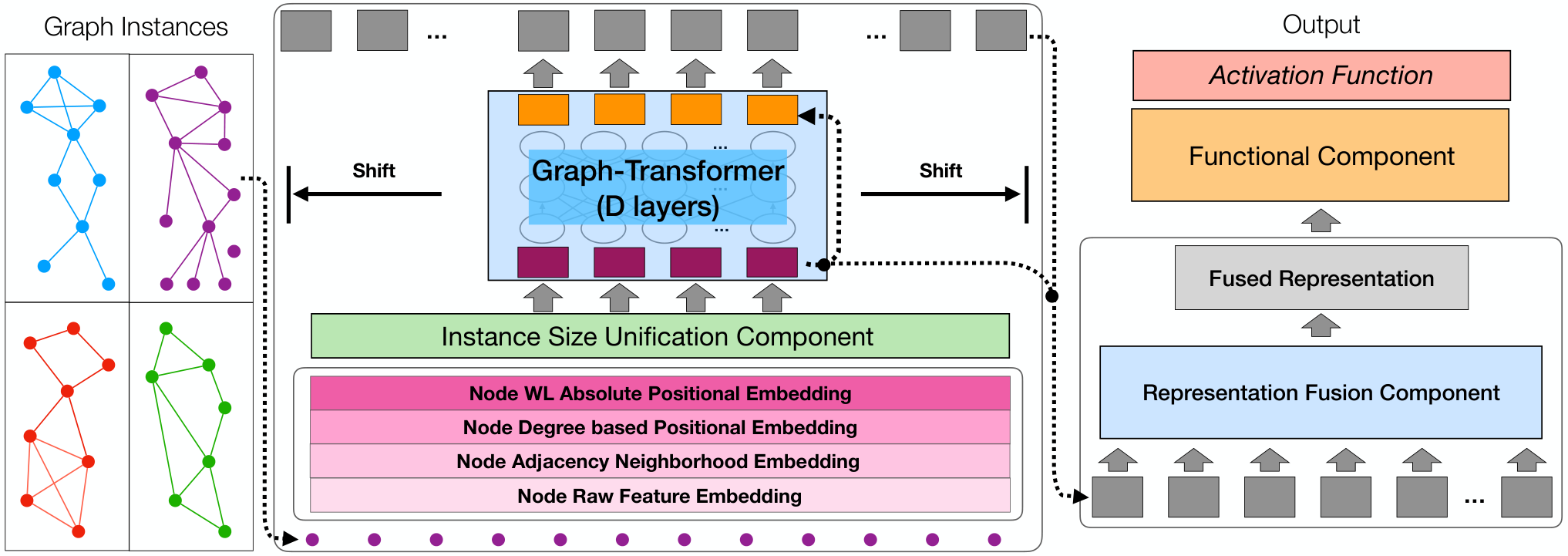
In this section, we will provide the detailed information about the Seg-Bert model for graph instance representation learning. As illustrated in Figure 1, the Seg-Bert model has several key components: (1) graph instance serialization to reshape the various-sized input graph instances into node list, where the node orders will not affect the learning results; (2) initial embedding extraction to define the initial input feature vectors for all nodes in the graph instance; (3) input size unification to fit the input portal size of graph-transformer; (4) graph-transformer to learn the nodes’ representations in the graph instance (or segments) with several layers; (5) representation fusion to integrate the learned representations of all nodes in the graph instance; and (6) functional component to compute and output the learning results. These components will all be introduced in this section in detail, whereas the learning detail of Seg-Bert will be discussed in the follow-up Section 5 instead.
4.1 Graph Serialization and Initial Embeddings
Formally, given a graph instance from the graph set, we can denote its structure as , involving node set and link set , respectively. To simplify the notations, we will not indicate the graph instance index subscript in this section. Both the initial inputs and the functional components in Seg-Bert are node-order-invariant, i.e., the nodes’ learned representations are not dependent on the node orders. Therefore, regardless of the nodes’ orders, we can serialize node set into a sequence . For the same graph instance, if it is fed to train/tune Seg-Bert for multiple times, the node order in the list can change arbitrarily without affecting the learning representations.
For each node in the list, e.g., , we can represent its raw features as a vector , which can cover various types of information, e.g., node tags, attributes, textual descriptions and even images. Via certain embedding mappings, we can denote the embedded feature representation of ’s raw features as
| (1) |
Depending on the input features, different approaches can be utilized to define the function, e.g., CNN for image features, LSTM for textual features, positional embedding for tags and MLP for real-number features. In the case when the graph instance nodes have no raw attributes on nodes, a dummy zero vector will be used to fill in the embedding vector entries by default.
To handle the graph instances without node attributes, in this paper, we will also extend the original Graph-Bert model by defining the node adjacency neighborhood embeddings. Meanwhile, to ensure such an embedding is node-order invariant, we will cast an artificially fixed node order on this embedding vector (which is fixed forever for the graph instance). For simplicity, we will just follow the node subscript index as the node orders in this paper. Formally, for each node , following the fixed artificial node order, we can denote its adjacency neighbors as a vector . Via several fully connected (FC) layers based mappings, we can represent the embedded representation of ’s adjacency neighborhood information as
| (2) |
The degrees of nodes can illustrate their basic properties (Chung et al. 2003; Bondy 1976), and according to (Lovász 1996) for the Markov chain or random walk on graphs, their final stationary distribution will be proportional to the nodes’ degrees. Node degree is also a node-order invariant actually. Formally, we can represent the degree of in the graph instance as , and its embedding can be represented as
| (3) | ||||
where and the vector index will iterate through the vector to compute the entry values based on the and functions.
In addition to the node raw feature embedding, node adjacency neighborhood embedding and node degree embedding, we will also include the nodes’ Weisfeiler-Lehman role embedding vector in this paper, which effectively denotes the nodes’ global roles in the input graph. Nodes’ Weisfeiler-Lehman code is node-order-invariant, which denotes a positional property of the nodes actually. Formally, given a node in the input graph instance, we can denote its pre-computed WL code as , whose corresponding embeddings can be denoted as
| (4) |
Seg-Bert doesn’t include the relative positional embedding and relative hop distance embedding used in (Zhang et al. 2020), as there exist no target node for the graph instances studied in this paper. Based on the above descriptions, we can represent the initially computed input embedding vectors of node in graph as
| (5) |
4.2 Graph Instance Size Unification Strategies
Different from (Zhang et al. 2020), where the sampled sub-graphs all have the identical size, the graph instance input usually have different number of nodes instead. To handle such a problem, we design Seg-Bert with an instance size unification component in this paper. Formally, we can denote the input portal size of Seg-Bert used in this paper as , i.e., it can take the initial input embedding vectors of nodes at a time. Depending on the input graph instance sizes, Seg-Bert will define the parameter and handle the graph instances with different strategies:
- •
Full-Input Strategy: The input portal size of Seg-Bert is defined as the largest graph instance size in the dataset, and dummy node padding will be used to expand all graph instances to nodes (zero padding for the connections, raw attributes and other tags).
- •
Padding/Pruning Strategy: The input portal size of Seg-Bert is assigned with a value slightly above the graph instance average size. For the graph instance input with less than nodes, dummy node padding (zero padding) is used to expand the graph to nodes; whereas for larger input graph instances, a -node sub-graph (e.g., the first nodes) will be extracted from them and the remaining nodes will be pruned.
- •
Segment Shifting Strategy: A fixed input portal size will be pre-specified, which can be a very small number. For the graph instance input with node set , the nodes will be divided into segments, and dummy node padding will be used for the last segment if necessary. Seg-Bert will shift along the segments to learn all the nodes representations in the graph instances.
Generally, the full-input strategy will use all the input graph nodes for representation learning, but for a small-graph set with a few number of extremely large graph instance(s), a very large will be used in Seg-Bert, which may introduce unnecessary high time costs. The padding/pruning strategy balances the parameter among all the graph instances and can learn effective representations in an efficient way, but it may have information loss for the pruned parts of some graph instances. Meanwhile, the segment shifting strategy can balance between the full-input strategy and padding/pruning strategy, which fuses the graph instance global information for representation learning with a small model input portal. More experimental tests of such different graph instance size unification strategies will also be explored with experiments on real-world benchmark datasets to be introduced in Section 6.


4.3 Segmented Graph-Transformer
To learn the graph instance representations, we will introduce the segmented graph-transformer in this part to update such nodes’ representations iteratively with layers. Formally, based on the above descriptions, we can denote the current segment as , whose initial input embeddings can be denoted as and is defined in Equation (5). Depending on the different unification strategies adopted, the segment can denote all the graph nodes, pruned/padded node subset or the node segments, respectively. For the segmented graph-transformer, it will update the segment representations iteratively for each layer according to the following equation:
| (6) | ||||
where and denote the transformer (Vaswani et al. 2017) and graph residual terms (Zhang & Meng 2019), respectively. Here, we need to add some remarks on the graph residual terms used in the model. Different from (Zhang et al. 2020), which integrates the target node residual terms to all the nodes in the batch, (1) for the graph instances without any node attributes, the nodes adjacency neighborhood vectors will be used to compute the residual terms, and (2) we compute the graph residual term with the whole graph instance instead in this paper (not merely for the target node).
Such a process will iterate through all the segments of the input graph instance nodes, and the finally learned node representations can be denoted as . In this paper, for presentation simplicity, we just assume all the hidden layers are of the same dimension . Considering that we focus on learning the representations of the entire graph instance in this paper, Seg-Bert will integrate such node representations together to define the fused graph instance representation vector as follows:
| (7) |
Both vector and matrix will be outputted to the down-stream application tasks for the model training/tuning and graph instance representation learning, which will be introduced in the follow-up section in detail.
5 Seg-Bert Learning
In this part, we will focus on the pre-training and fine-tuning of Seg-Bert with several concrete graph instance learning tasks. To be more specific, we will introduce two unsupervised pre-training tasks to learn Seg-Bert based on node raw attribute reconstruction and graph structure recovery, which ensure the learned node and graph representations can capture both the raw attribute and structure information in the graph instances. After that, we will introduce one supervised tasks to fine-tune Seg-Bert for the graph instance classification, which will cast extra refinements on the learned node and graph representations.
5.1 Unsupervised Pre-Training
The pre-training tasks used in this paper will enable Seg-Bert to effectively capture both the node raw attributes and graph instance structures in the learned nodes and graph representation vectors. In the case where the graph instances have no node raw attributes, only graph structure recovery will be used for the pre-training. Formally, based on the learned representations of all the nodes in the graph instance, e.g., , with several fully connected layers, we can project such latent representations to their raw features. Furthermore, by comparing the reconstructed feature matrix against the ground-truth raw features and minimizing their differences, we will be able to pre-train the Seg-Bert model with all the graph instances. Furthermore, based on the nodes learned representations, we can also compute the closeness (e.g., cosine similarity of the representation vectors) of the node pairs in the graph. Furthermore, compared against the ground-truth graph connection weight matrix, we can define the introduced loss term for graph structure recovery of all the graph instances to pre-train the Seg-Bert model.
| Datasets | IMDB-B | IMDB-M | COLLAB | MUTAG | PROTEINS | PTC | NCI1 |
| # Graphs | 1,000 | 1,500 | 5,000 | 188 | 1,113 | 344 | 4,110 |
| # Classes | 2 | 3 | 3 | 2 | 2 | 3 | 2 |
| Avg. # Nodes | 19.8 | 13.0 | 74.5 | 17.9 | 39.1 | 25.5 | 29.8 |
| max # Nodes | 136 | 89 | 492 | 28 | 620 | 109 | 111 |
| Methods | Accuracy (meanstd) | ||||||
| WL (Shervashidze et al. 2011) | 73.404.63 | 49.334.75 | 79.021.77 | 82.050.36 | 74.680.49 | 59.904.30 | 82.190.18 |
| GK (Shervashidze et al. 2009) | 65.870.98 | 43.890.38 | 72.840.28 | 81.582.11 | 71.670.55 | 57.261.41 | 62.280.29 |
| DGK (Yanardag & Vishwanathan 2015) | 66.960.56 | 44.550.52 | 73.090.25 | 87.442.72 | 75.680.54 | 60.082.55 | 80.310.46 |
| AWE (Ivanov & Burnaev 2018) | 74.455.83 | 51.543.61 | 73.931.94 | 87.879.76 | |||
| PSCN (Niepert et al. 2016) | 71.002.29 | 45.232.84 | 72.602.15 | 88.954.37 | 75.002.51 | 62.295.68 | 76.341.68 |
| DAGCN (Chen et al. 2019) | 87.226.10 | 76.334.3 | 62.889.61 | 81.681.69 | |||
| SPI-GCN (Atamna et al. 2019) | 60.404.15 | 44.134.61 | 84.408.14 | 72.063.18 | 56.415.71 | 64.112.37 | |
| DGCNN (Zhang et al. 2018) | 70.030.86 | 47.830.85 | 73.760.49 | 85.831.66 | 75.540.94 | 58.592.47 | 74.440.47 |
| GCAPS-CNN (Verma & Zhang 2018) | 71.693.40 | 48.504.10 | 77.712.51 | 76.404.17 | 66.015.91 | 82.722.38 | |
| CapsGNN (Zhang & Chen 2019) | 73.104.83 | 50.272.65 | 79.620.91 | 86.676.88 | 76.283.63 | 78.351.55 | |
| Seg-Bert(padding/pruning, none) | 75.402.29 | 52.271.55 | 78.421.29 | 89.247.78 | 77.094.15 | 68.864.17 | 70.151.84 |
| Seg-Bert(padding/pruning, raw) | 74.703.74 | 50.603.03 | 74.901.78 | 89.806.71 | 76.282.91 | 64.846.77 | 68.102.55 |
| Seg-Bert* | 77.203.09 | 53.402.12 | 78.421.29 | 90.856.58 | 77.094.15 | 68.864.17 | 70.151.84 |
5.2 Transfer and Fine-Tuning
When applying the pre-trained Seg-Bert and the learned representations in new application tasks, e.g., graph instance classification, necessary fine-tuning can be needed. Formally, we can denote the batch of labeled graph instance as , where denotes the label vector of graph instance . Based on the fused representation vector learned for graph instance , we can further project it to the label vector with several fully connected layers together with the softmax normalization function, which can be denoted as
| (8) |
Meanwhile, based on the known ground-truth label vector of graph instances in the training set, we can define the introduced loss term for the graph instance based on the corss-entropy term as follows:
| (9) |
By optimizing the above loss term, we will be able to re-fine Seg-Bert and the learned graph instance representations based on the application tasks specifically.
6 Experiments
To test the effectiveness of Seg-Bert, extensive experiments on real-world graph instance benchmark datasets will be done in this section. What’s more, we will also compare Seg-Bert with both the classic and state-of-the-art graph instance representation learning baseline methods to demonstrate its advantages.
Reproducibility: Both the datasets and source code used can be accessed via the github page11 1 https://github.com/jwzhanggy/SEG-BERT. Detailed information about the server used to run the model can be found at the footnote22 2 GPU Server: ASUS X99-E WS motherboard, Intel Core i7 CPU 6850K@3.6GHz (6 cores, 40 PCIe lanes), 3 Nvidia GeForce GTX 1080 Ti GPU (11 GB buffer each), 128 GB DDR4 memory and 128 GB SSD swap..
| Strategies | IMDB-B | IMDB-M | MUTAG | PTC | ||||||||
|---|---|---|---|---|---|---|---|---|---|---|---|---|
| Accuracy | k | Time(s) | Accuracy | k | Time(s) | Accuracy | k | Time(s) | Accuracy | k | Time(s) | |
| Full-Input | 76.901.76 | 136 | 2808.70 | 53.332.53 | 89 | 2397.42 | 90.856.58 | 28 | 55.73 | 68.014.23 | 109 | 700.98 |
| Padding/Pruning | 75.402.29 | 50 | 1312.42 | 52.271.55 | 50 | 1654.66 | 89.247.78 | 25 | 55.19 | 68.864.17 | 50 | 223.47 |
| Segment Shifting | 77.203.09 | 20 | 1525.97 | 53.402.12 | 20 | 1730.08 | 90.297.74 | 20 | 88.40 | 66.544.18 | 20 | 295.83 |
6.1 Dataset and Experimental Settings
Dataset Descriptions: The graph instance datasets used in this experiments include IMDB-Binary, IMDB-Multi and COLLAB, as well as MUTAG, PROTEINS, PTC and NCI1, which are all the benchmark datasets as used in (Yanardag & Vishwanathan 2015) and all the follow-up graph classification papers (Zhang & Chen 2019; Verma & Zhang 2018; Xu et al. 2018). Among them, IMDB-Binary, IMDB-Multi and COLLAB are the social graph datasets; whereas the remaining ones are the bio-graph datasets. Basic statistical information about the datasets is also available at the top of Table 1.
Comparison Baselines: The comparison baseline methods used in this paper include (1) conventional graph kernel based methods, e.g., Weisfeiler-Lehman subtree kernel (WL) (Shervashidze et al. 2011) and graphlet count kernel (GK) (Shervashidze et al. 2009); (2) existing deep learning based methods, e.g., Deep Graph Kernel (DGK) (Yanardag & Vishwanathan 2015) and AWE (Ivanov & Burnaev 2018), PATCHY-SAN (PSCN) (Niepert et al. 2016); and (3) state-of-the-art deep learning methods, e.g., Dual Attention Graph Convolutional Network (DAGCN) (Chen et al. 2019), Simple Permutation-Invariant Graph Convolutional Network (SPI-GCN) (Atamna et al. 2019), Graph Capsule CNN (GCAPS-CNN) (Verma & Zhang 2018) and Deep Graph CNN (DGCNN) (Zhang et al. 2018), and Capsule Graph Neural Network (CapsGNN) (Zhang & Chen 2019). Evaluation Metric: The learning performance of these methods will be evaluated by Accuracy as the metric.
Experimental Settings: In the experiments, we will first compare Seg-Bert with the padding/pruning strategy for input size unification against the baseline methods, which can help test if a sub-structures in graph instances can capture the characteristics of the whole graph instance or not. The other two strategies will be discussed at the end of this section in detail. For the input portal size , it is assigned with a value slightly larger than the graph instance average sizes of each dataset. All the graph instances in the datasets will be partitioned into train, validate, testing sets according to the ratio 8:1:1 with the -fold cross validation, where the validation set is used for parameter tuning and selection. Meanwhile, for fair comparisons (existing works use train/test partition without validation set), such validation set will also be used as training data as well to further fine-tune Seg-Bert after the parameter selection.
Default Model Parameter Settings: If not clearly specified, the results reported in this paper are based on the following parameter settings of Seg-Bert: input portal size: (MUTAG), (IMDB-Binary, IMDB-Multi, NCI1, PTC) and (COLLAB, PROTEINS); hidden size: 32; attention head number: 2; hidden layer number: ; learning rate: 0.0005 (PTC) and 0.0001 (others); weight decay: ; intermediate size: 32; hidden dropout rate: 0.5; attention dropout rate: 0.3; graph residual term: raw/none; training epoch: 500 (early stop if necessary to avoid over-fitting).
6.2 Graph Instance Classification Results
Model Train Records: As illustrated in Figure 2, we show the learning records (training/testing accuracy) of Seg-Bert on both the IMDB-Multi social graph and the Protein bio-graph datasets. According to the plots, graph instance classification is very different from classification task on other data types, as the model can get over-fitting easily. Similar phenomena have been observed for most comparison methods on the other datasets as well. Even though the default training epoch is mentioned above, an early stop of training Seg-Bert is usually necessary. In this paper, we decide the early-stop learning epoch number based on the partitioned validation set.
Main Results: The main learning results of of all the comparison methods are provided in Table 1. The Seg-Bert method shown here adopts the padding/pruning strategy to handle the graph data input. The residual terms adopted are indicated by the Seg-Bert method name in the parentheses. According to the evaluation results, Seg-Bert can greatly improve the learning performance on most of the benchmark datasets. For instance, the accuracy score of Seg-Bert (none) on IMDB-Binary is , which is much higher than many of the state-of-the-art baseline methods, e.g., DGCNN, GCAPS-CNN and CapsGNN. Similarly learning performance advantages have also been observed on the other datasets, except NCI1.
For the raw residual term used in Seg-Bert, for some of the datasets as shown in Table 1, e.g., MUTAG, it can improve the learning performance; whereas for the remaining ones, its effectiveness is not very significant. The main reason can be for most of the graph instances studied here they don’t have node attributes and the discrete nodes adjacency neighborhood embeddings can be very sparse, which renders the computed residual terms to be less effective for performance improvement.
Graph Size Unification Strategy Analysis: The analyses of the different graph size unification strategies is provided in Table 2. For Seg-Bert with the full-input strategy on COLLAB, PROTEIN and NCI1 (with more instances and large max graph sizes), the training time costs are too high ( 3 days to run the 10 folds). So, the results on these three datasets are not shown here. As illustrated in Table 2, the performance of full-input is better than padding/pruning, but it also consumes the highest time cost. The padding/pruning strategy has the lowest time costs but its performance is slightly lower than full-input and segment shifting. Meanwhile, the learning performance of segment shifting balances between full-input and padding/pruning, which can even out-perform full-input as it introduce far less dummy paddings in the input.
7 Conclusion
In this paper, we have introduce a new graph neural network model, namely Seg-Bert, for graph instance representation learning. With several significant modifications, the re-designed Seg-Bert has no node-order-variant inputs or function components, which can handle the node orderless property very well. Seg-Bert has an extendable architecture. For large-sized graph instance input, Seg-Bert will divide the nodes into segments, whereas all the nodes in the graph will be used for the representation learning of each segment. We have tested the effectiveness of Seg-Bert on several concrete application tasks, and the experimental results demonstrate that Seg-Bert can out-perform the state-of-the-art graph instance representation learning models effectively.
References
- Atamna et al. (2019) Atamna, A., Sokolovska, N., and CRIVELLO, J.-C. SPI-GCN: A Simple Permutation-Invariant Graph Convolutional Network. working paper or preprint, April 2019. URL https://hal.archives-ouvertes.fr/hal-02093451.
- Bondy (1976) Bondy, J. A. Graph Theory With Applications. Elsevier Science Ltd., GBR, 1976. ISBN 0444194517.
- Chen et al. (2019) Chen, F., Pan, S., Jiang, J., Huo, H., and Long, G. DAGCN: dual attention graph convolutional networks. CoRR, abs/1904.02278, 2019. URL http://arxiv.org/abs/1904.02278.
- Chung et al. (2003) Chung, F., Lu, L., and Vu, V. Spectra of random graphs with given expected degrees. Proceedings of the National Academy of Sciences, 100(11):6313–6318, 2003. ISSN 0027-8424. doi: 10.1073/pnas.0937490100. URL https://www.pnas.org/content/100/11/6313.
- Chung et al. (2014) Chung, J., Gülçehre, Ç., Cho, K., and Bengio, Y. Empirical evaluation of gated recurrent neural networks on sequence modeling. CoRR, abs/1412.3555, 2014. URL http://arxiv.org/abs/1412.3555.
- Defferrard et al. (2016) Defferrard, M., Bresson, X., and Vandergheynst, P. Convolutional neural networks on graphs with fast localized spectral filtering. In Lee, D. D., Sugiyama, M., Luxburg, U. V., Guyon, I., and Garnett, R. (eds.), Advances in Neural Information Processing Systems 29, pp. 3844–3852. Curran Associates, Inc., 2016.
- Devlin et al. (2018) Devlin, J., Chang, M., Lee, K., and Toutanova, K. BERT: pre-training of deep bidirectional transformers for language understanding. CoRR, abs/1810.04805, 2018. URL http://arxiv.org/abs/1810.04805.
- Hammond et al. (2011) Hammond, D. K., Vandergheynst, P., and Gribonval, R. Wavelets on graphs via spectral graph theory. Applied and Computational Harmonic Analysis, 30(2):129?150, Mar 2011. ISSN 1063-5203. doi: 10.1016/j.acha.2010.04.005. URL http://dx.doi.org/10.1016/j.acha.2010.04.005.
- Hochreiter & Schmidhuber (1997) Hochreiter, S. and Schmidhuber, J. Long short-term memory. Neural Comput., 9(8), November 1997.
- Ivanov & Burnaev (2018) Ivanov, S. and Burnaev, E. Anonymous walk embeddings. CoRR, abs/1805.11921, 2018. URL http://arxiv.org/abs/1805.11921.
- Jiang et al. (2018) Jiang, J., Cui, Z., Xu, C., and Yang, J. Gaussian-induced convolution for graphs. CoRR, abs/1811.04393, 2018. URL http://arxiv.org/abs/1811.04393.
- Kim (2014) Kim, Y. Convolutional neural networks for sentence classification. In Proceedings of the 2014 Conference on Empirical Methods in Natural Language Processing (EMNLP), pp. 1746–1751, Doha, Qatar, October 2014. Association for Computational Linguistics. doi: 10.3115/v1/D14-1181. URL https://www.aclweb.org/anthology/D14-1181.
- Kipf & Welling (2016) Kipf, T. N. and Welling, M. Semi-supervised classification with graph convolutional networks. CoRR, abs/1609.02907, 2016.
- Kriege et al. (2016) Kriege, N. M., Giscard, P.-L., and Wilson, R. On valid optimal assignment kernels and applications to graph classification. In Lee, D. D., Sugiyama, M., Luxburg, U. V., Guyon, I., and Garnett, R. (eds.), Advances in Neural Information Processing Systems 29, pp. 1623–1631. Curran Associates, Inc., 2016.
- Krizhevsky et al. (2012) Krizhevsky, A., Sutskever, I., and Hinton, G. E. Imagenet classification with deep convolutional neural networks. In Pereira, F., Burges, C. J. C., Bottou, L., and Weinberger, K. Q. (eds.), Advances in Neural Information Processing Systems 25, pp. 1097–1105. Curran Associates, Inc., 2012.
- Liu et al. (2019) Liu, Y., Ott, M., Goyal, N., Du, J., Joshi, M., Chen, D., Levy, O., Lewis, M., Zettlemoyer, L., and Stoyanov, V. Roberta: A robustly optimized BERT pretraining approach. CoRR, abs/1907.11692, 2019. URL http://arxiv.org/abs/1907.11692.
- Lovász (1996) Lovász, L. Random walks on graphs: A survey. In Miklós, D., Sós, V. T., and Szőnyi, T. (eds.), Combinatorics, Paul Erdős is Eighty, volume 2, pp. 353–398. János Bolyai Mathematical Society, Budapest, 1996.
- Mallea et al. (2019) Mallea, M. D. G., Meltzer, P., and Bentley, P. J. Capsule neural networks for graph classification using explicit tensorial graph representations. CoRR, abs/1902.08399, 2019. URL http://arxiv.org/abs/1902.08399.
- Meltzer et al. (2019) Meltzer, P., Mallea, M. D. G., and Bentley, P. J. Pinet: A permutation invariant graph neural network for graph classification. CoRR, abs/1905.03046, 2019. URL http://arxiv.org/abs/1905.03046.
- Meng & Zhang (2019) Meng, L. and Zhang, J. Isonn: Isomorphic neural network for graph representation learning and classification. CoRR, abs/1907.09495, 2019. URL http://arxiv.org/abs/1907.09495.
- Narayanan et al. (2017) Narayanan, A., Chandramohan, M., Venkatesan, R., Chen, L., Liu, Y., and Jaiswal, S. graph2vec: Learning distributed representations of graphs. CoRR, abs/1707.05005, 2017. URL http://arxiv.org/abs/1707.05005.
- Niepert et al. (2016) Niepert, M., Ahmed, M., and Kutzkov, K. Learning convolutional neural networks for graphs. CoRR, abs/1605.05273, 2016. URL http://arxiv.org/abs/1605.05273.
- Raffel et al. (2019) Raffel, C., Shazeer, N., Roberts, A., Lee, K., Narang, S., Matena, M., Zhou, Y., Li, W., and Liu, P. J. Exploring the limits of transfer learning with a unified text-to-text transformer. arXiv preprint arXiv:1910.10683, 2019.
- Ranjan et al. (2019) Ranjan, E., Sanyal, S., and Talukdar, P. P. Asap: Adaptive structure aware pooling for learning hierarchical graph representations. arXiv preprint arXiv:1911.07979, 2019.
- Shervashidze et al. (2009) Shervashidze, N., Vishwanathan, S., Petri, T., Mehlhorn, K., and Borgwardt, K. Efficient graphlet kernels for large graph comparison. In van Dyk, D. and Welling, M. (eds.), Proceedings of the Twelth International Conference on Artificial Intelligence and Statistics, volume 5 of Proceedings of Machine Learning Research, pp. 488–495, Hilton Clearwater Beach Resort, Clearwater Beach, Florida USA, 16–18 Apr 2009. PMLR. URL http://proceedings.mlr.press/v5/shervashidze09a.html.
- Shervashidze et al. (2011) Shervashidze, N., Schweitzer, P., van Leeuwen, E. J., Mehlhorn, K., and Borgwardt, K. M. Weisfeiler-lehman graph kernels. J. Mach. Learn. Res., 12(null):2539?2561, November 2011. ISSN 1532-4435.
- Sun et al. (2019) Sun, Y., Wang, S., Li, Y., Feng, S., Tian, H., Wu, H., and Wang, H. ERNIE 2.0: A continual pre-training framework for language understanding. CoRR, abs/1907.12412, 2019. URL http://arxiv.org/abs/1907.12412.
- Vaswani et al. (2017) Vaswani, A., Shazeer, N., Parmar, N., Uszkoreit, J., Jones, L., Gomez, A. N., Kaiser, L., and Polosukhin, I. Attention is all you need. CoRR, abs/1706.03762, 2017. URL http://arxiv.org/abs/1706.03762.
- Veličković et al. (2018) Veličković, P., Cucurull, G., Casanova, A., Romero, A., Liò, P., and Bengio, Y. Graph Attention Networks. International Conference on Learning Representations, 2018.
- Verma & Zhang (2018) Verma, S. and Zhang, Z.-L. Graph capsule convolutional neural networks. arXiv preprint arXiv:1805.08090, 2018.
- Xu et al. (2018) Xu, K., Hu, W., Leskovec, J., and Jegelka, S. How powerful are graph neural networks? CoRR, abs/1810.00826, 2018. URL http://arxiv.org/abs/1810.00826.
- Yanardag & Vishwanathan (2015) Yanardag, P. and Vishwanathan, S. Deep graph kernels. In Proceedings of the 21th ACM SIGKDD International Conference on Knowledge Discovery and Data Mining, KDD ?15, pp. 1365?1374, New York, NY, USA, 2015. Association for Computing Machinery. ISBN 9781450336642. doi: 10.1145/2783258.2783417. URL https://doi.org/10.1145/2783258.2783417.
- Zhang (2019) Zhang, J. Graph Neural Networks for Small Graph and Giant Network Representation Learning: An Overview. arXiv e-prints, art. arXiv:1908.00187, Jul 2019.
- Zhang & Meng (2019) Zhang, J. and Meng, L. Gresnet: Graph residual network for reviving deep gnns from suspended animation. ArXiv, abs/1909.05729, 2019.
- Zhang et al. (2020) Zhang, J., Zhang, H., Sun, L., and Xia, C. Graph-bert: Only attention is needed for learning graph representations. arXiv preprint arXiv:2001.05140, 2020.
- Zhang et al. (2018) Zhang, M., Cui, Z., Neumann, M., and Chen, Y. An end-to-end deep learning architecture for graph classification. In AAAI, 2018.
- Zhang & Chen (2019) Zhang, X. and Chen, L. Capsule graph neural network. In International Conference on Learning Representations, 2019. URL https://openreview.net/forum?id=Byl8BnRcYm.