跳到论文正文
W Papers独立论文阅读器 arXiv:2002.03209 论文正文 计算阅读时间 · 0%
引用这篇论文根据当前论文元数据生成,正式投稿前建议核对。


License: arXiv.org perpetual non-exclusive license
arXiv:2002.03209v1 [eess.SP] 08 Feb 2020

Affine Combination of Diffusion Strategies
over Networks

Danqi Jin       Jie Chen       Cédric Richard       Jingdong Chen       Ali H. Sayed    Thanks: D. Jin, J. Chen and J. Chen are with Centre of Intelligent Acoustics and Immersive Communications at School of Marine Science and Technology, Northwestern Polytechinical University, Xi’an, China (emails: danqijin@mail.nwpu.edu.cn, dr.jie.chen@ieee.org, jingdongchen@ieee.org). C. Richard is with Université Côte d’Azur, CNRS, France (email: cedric.richard@unice.fr). A. H. Sayed is with the School of Engineering, Ećole Polytechnique Fédérale de Lausanne (EPFL), Switzerland (email: ali.sayed@epfl.ch). The work of C. Richard was funded in part by ANR under grant ANR-19-CE48-0002.
Abstract

Diffusion adaptation is a powerful strategy for distributed estimation and learning over networks. Motivated by the concept of combining adaptive filters, this work proposes a combination framework that aggregates the operation of multiple diffusion strategies for enhanced performance. By assigning a combination coefficient to each node, and using an adaptation mechanism to minimize the network error, we obtain a combined diffusion strategy that benefits from the best characteristics of all component strategies simultaneously in terms of excess-mean-square error (EMSE). Analyses of the universality are provided to show the superior performance of affine combination scheme and to characterize its behavior in the mean and mean-square sense. Simulation results are presented to demonstrate the effectiveness of the proposed strategies, as well as the accuracy of theoretical findings.

Index Terms: 
Distributed optimization, diffusion strategy, affine combination, adaptive fusion strategy, stochastic performance.

I INTRODUCTION

Distributed adaptive algorithms endow networks with the ability to estimate and track unknown parameters from streaming data in a collaborative manner. Typical existing techniques include consensus, incremental and diffusion strategies [1, 2, 3, 4, 5, 6]. Diffusion strategies have been shown to have superior performance in adaptive scenarios where it is necessary to track drifts in the underlying models through constant step-size adaptation [7]. There are many variants of diffusion schemes, including diffusion LMS and its multitask counterparts [8, 9, 10], diffusion APA [11], diffusion RLS [12]. In this work, we focus on diffusion techniques due to their enhanced adaptation performance and wider stability ranges.

Diffusion algorithms typically consist of an adaptation step and a combination step. In the adaptation step, each agent updates its iterate by using a local gradient approximation. In the combination step, each agent collects intermediate estimates from its neighbors and fuses them with proper weights. The proper selection of the fusion weights is important for enhanced performance. However, finding an optimal setting for these weights is generally non-trivial. Several empirical strategies with fixed coefficients have been proposed, including averaging rule, Metropolis rule and relative-degree rule[5]. Adaptive strategies have also been derived by considering noise levels across the network [13], or relationships among agents [9]. Given that different strategies tend to deliver varying performance levels under different operating conditions, it is worth examining the possibility of combining strategies to extract the best performance possible. For example, it is useful to examine whether it is possible to combine two distributed strategies and obtain a new strategy whose performance is superior to its individual components. The question was answered in the affirmative for stand-alone adaptive filters in [14, 15, 16]. It is more challenging in the context of adaptive networks with a multitude of interacting agents over a graph. We will show nevertheless that this is still possible.

Combination strategies have been successfully used for classical adaptive filters [14, 17], multi-kernel learning [18], as well as modern deep neural network structures [19]. It is shown in some of these works that using convex combinations [17, 14] or affine combinations [20] of adaptive filters with diversity can lead to filters that combine the advantages of all component filters. Generally, such combination schemes are used to facilitate the selection of filter parameters, to increase robustness against an unknown environment, or to possibly enhance performance beyond the range of each component [15]. In this paper, we propose affine combination schemes for diffusion strategies. Each agent is designed to run several diffusion strategies in parallel, and to combine their estimates to generate the final estimates. Time-varying affine combination coefficients are set by minimizing the overall squared instantaneous error. Simulation results show that the proposed algorithms endow the networks with a significantly enhanced performance in the learning process. Some related works can be found in [21] and our previous work [22]. In [21], the authors use a useful convex combination scheme for combining two specific fusion strategies albeit without motivating it or formulating a driving optimization problem. Though similar to [21], in [22] a convex combination scheme is proposed for two diffusion strategies. However, both works do not examine the theoretical underpinnings of the algorithms. We should also note that the work proposed here is different from the useful formulation in [23]. This last reference introduces a diffusion scheme for networks with heterogeneous nodes, namely, nodes implementing different adaptive rules or differing in other aspects such as filter structure, length or step-size. In comparison, our work proposes affine combination schemes to combine different diffusion strategies, which can be either homogeneous or heterogeneous. In that sense, the results presented here are more general than [23].

The main contributions of this work are summarized as follows:

  • •

    We introduce a framework for the affine combination of two component diffusion algorithms over networks, and propose two methods for adjusting the combination weights. The framework can be extended to multiple component algorithms as explained in Appendix A.

  • •

    We establish the universality of the combined strategy, in a manner that extends a prior universality analysis for the combination of adaptive filters.

  • •

    We conduct a theoretical analysis of the performance of combined diffusion LMS strategies under some typical simplifying assumptions and approximations. Although the assumptions are not accurate in general, they are nevertheless typical in the context of studying adaptive systems and tend to lead to performance results that match well with practice for sufficiently small step-sizes with white measurement noise and white regressors [24].

Notation. Normal font xx denotes scalars. Boldface small letters 𝒙\bm{x} and capital letters 𝑿{\bm{X}} denote column vectors and matrices, respectively. The superscript (⋅)⊤{(\cdot)}^{\top} denotes the transpose operator. The inverse of a square matrix is denoted by (⋅)−1{(\cdot)}^{-1}. The mathematical expectation is denoted by 𝔼​{⋅}{\mathbb{E}}\{\cdot\}. The Gaussian distribution with mean μ\mu and variance σ2\sigma^{2} is denoted by 𝒩⁡(μ,σ2){\mathcal{N}}(\mu,\sigma^{2}). The operators min⁡{⋅}\min\{\cdot\} and max⁡{⋅}\max\{\cdot\} return the minimal or maximal value of their arguments. The operator diag​{⋅}\text{diag}\{\cdot\} extracts the diagonal elements of its matrix argument, or generates a diagonal matrix from its vector argument. The operator |⋅||\cdot| returns the absolute value of its argument. 𝑰N\bm{I}_{N} and 𝟎N\bm{0}_{N} denote identity matrix and zero matrix of size N×NN\times N, respectively. All-one vector of length NN is denoted by 𝟙N\mathbbm{1}_{N}. Symbol 𝒞i{\cal C}_{i} stands for cluster ii, i.e., index set of nodes in the ii-th cluster. 𝒩k{\cal{N}}_{k} denotes the neighbors of node kk, including kk.

II NETWORK MODEL AND DIFFUSION LMS

II-A Network Model

Consider a connected network consisting of NN agents. The problem is to estimate an unknown parameter vector 𝒘k⋆\bm{w}_{k}^{\star} of length L×1L\times 1 at each agent kk. Agent kk has access to temporal measurement sequences {dk,n,𝒙k,n}\{d_{k,n},\bm{x}_{k,n}\}, where dk,nd_{k,n} denotes a reference signal, and 𝒙k,n\bm{x}_{k,n} is an L×1L\times 1 regression vector with positive-definite covariance matrix. The data at agent kk and time instant nn are driven by the linear model:

dk,n=𝒙k,n⊤​𝒘k⋆+zk,n,d_{k,n}=\bm{x}^{\top}_{k,n}\bm{w}_{k}^{\star}+z_{k,n}, (1)

where zk,nz_{k,n} is an additive noise. For ease of derivation, we introduce the following assumption A111 1 In this paper, we adopt the acronym “A” for “assumption”. for zk,nz_{k,n}. Although rarely true in practice, A1 simplifies the derivation of algorithm and theoretical analysis, thus it is widely adopted in the context of online learning and adaptation [5, 6].

A1: The additive noise zk,nz_{k,n} is zero-mean, stationary, independent and identically distributed (i.i.d.) with variance σz,k2\sigma_{z,k}^{2}, and independent of any other signal.

To determine the unknown parameter vector 𝒘k⋆\bm{w}_{k}^{\star}, we consider the following mean-square-error (MSE) cost at agent kk:

Jk​(𝒘)=𝔼⁡{|dk,n−𝒙k,n⊤​𝒘|2}.J_{k}(\bm{w})={\mathbb{E}}\big\{|d_{k,n}-\bm{x}^{\top}_{k,n}\bm{w}|^{2}\big\}. (2)

Observe in (1) that Jk​(𝒘)J_{k}(\bm{w}) is minimized at 𝒘k⋆\bm{w}_{k}^{\star}. For single-task problems, each agent in the network estimates the same parameter vector, while for multi-task problems, agents may estimate distinct parameter vectors [8].

II-B Diffusion LMS Algorithm

The diffusion LMS algorithm is derived to minimize the following aggregate cost function:

Jglob​(𝒘)=∑k=1NJk​(𝒘)J^{\text{glob}}(\bm{w})=\sum_{k=1}^{N}J_{k}(\bm{w}) (3)

in a cooperative manner. The general structure of the diffusion LMS algorithm consists of the following steps:

ϕk,n\displaystyle{\bm{\phi}}_{k,n} =∑ℓ∈𝒩ka1,ℓ​k​𝒘ℓ,n,\displaystyle=\sum_{\ell\in{\cal{N}}_{k}}a_{1,\ell k}\,{\bm{w}}_{\ell,n}, (4)
𝝍k,n+1\displaystyle{\bm{\psi}}_{k,n+1} =ϕk,n+μk​∑ℓ∈𝒩kcℓ​k​𝒙ℓ,n​(dℓ,n−𝒙ℓ,n⊤​ϕk,n),\displaystyle={\bm{\phi}}_{k,n}+\mu_{k}\,\sum_{\ell\in{\cal{N}}_{k}}c_{\ell k}\,\bm{x}_{\ell,n}\,(d_{\ell,n}-\bm{x}^{\top}_{\ell,n}\,{\bm{\phi}}_{k,n}), (5)
𝒘k,n+1\displaystyle\bm{w}_{k,n+1} =∑ℓ∈𝒩ka2,ℓ​k​𝝍ℓ,n+1,\displaystyle=\sum_{\ell\in{\cal{N}}_{k}}a_{2,\ell k}\,{\bm{\psi}}_{\ell,n+1}, (6)

where 𝒘k,n+1\bm{w}_{k,n+1}, 𝝍k,n+1{\bm{\psi}}_{k,n+1} and ϕk,n{\bm{\phi}}_{k,n} are estimates for the unknown parameter vectors 𝒘k⋆\bm{w}_{k}^{\star} obtained at different operating stages of the diffusion algorithm, with subscripts kk and nn denoting node index and time index, respectively, and μk>0\mu_{k}>0 is the step-size at node kk, the nonnegative coefficients a1,ℓ​k,a2,ℓ​ka_{1,\ell k},a_{2,\ell k} and cℓ​kc_{\ell k} are the (ℓ,k)(\ell,k)-th entries of two left stochastic matrices 𝑨1,𝑨2\bm{A}_{1},\bm{A}_{2} and a right stochastic matrix 𝑪\bm{C}, respectively, satisfying:

𝑨1⊤​𝟙N=𝟙N,𝑨2⊤​𝟙N=𝟙N,𝑪​𝟙N=𝟙N,\displaystyle\bm{A}_{1}^{\top}\mathbbm{1}_{N}=\mathbbm{1}_{N},\,\bm{A}_{2}^{\top}\mathbbm{1}_{N}=\mathbbm{1}_{N},\,\bm{C}\mathbbm{1}_{N}=\mathbbm{1}_{N}, (7)
a1,ℓ​k=0,a2,ℓ​k=0,cℓ​k=0​if​ℓ∉𝒩k.\displaystyle a_{1,\ell k}=0,\;\;a_{2,\ell k}=0,\;\;c_{\ell k}=0\;\;{\rm{if}}\;\;\ell\notin{\cal{N}}_{k}. (8)

Several adaptive strategies can be obtained as special cases of (4) to (6). Two popular strategies, namely, adapt-then-combine (ATC) and combine-then-adapt (CTA), can be achieved by setting 𝑨1=𝑰N\bm{A}_{1}=\bm{I}_{N} and 𝑨2=𝑰N\bm{A}_{2}=\bm{I}_{N} respectively.

III GENERAL COMBINATION FRAMEWORK

III-A Combination framework

Combining two diffusion strategies can be performed with two concurrent adaptive layers: a diffusion strategy layer and a combination layer. The diffusion strategy layer consists of a distributed network running two distinct diffusion strategies, say S(1){\rm S}^{(1)} and S(2){\rm S}^{(2)}, individually and simultaneously, with associated quantities denoted by 𝑨1(i),𝑨2(i),𝑪(i),μ(i)\bm{A}_{1}^{(i)},\bm{A}_{2}^{(i)},\bm{C}^{(i)},\mu^{(i)}, where the superscript (i) denotes the ii-th component diffusion strategy S(i){\rm S}^{(i)} with i=1,2i=1,2. The scheme is illustrated in Fig. 1. In S(1){\rm S}^{(1)} and S(2){\rm S}^{(2)}, the agents have access to identical input and reference signals, and produce each an individual estimate of the optimal weight vector. We associate the combination coefficients γk,n\gamma_{k,n} and 1−γk,n1-\gamma_{k,n}, to S(1){\rm S}^{(1)} and S(2){\rm S}^{(2)}, respectively, at each agent kk and time instant nn. The goal of the combination layer is to learn which diffusion strategy performs better at each time instant, by adjusting γk,n\gamma_{k,n} in order to optimize the overall network performance.

Refer to caption

Fig. 1: Illustration of the combination framework for two diffusion strategies.

For each S(i){\rm S}^{(i)}, we define the filter output yk,n(i)y_{k,n}^{(i)}, the estimation error ek,n(i)e_{k,n}^{(i)}, and the a priori output estimation error e~k,n(i)\widetilde{e}_{k,n}^{(i)}:

yk,n(i)\displaystyle y_{k,n}^{(i)} ≜𝒙k,n⊤​𝒘k,n(i),\displaystyle\triangleq\bm{x}_{k,n}^{\top}\,{\bm{w}}_{k,n}^{(i)}, (9)
ek,n(i)\displaystyle e_{k,n}^{(i)} ≜dk,n−𝒙k,n⊤​𝒘k,n(i),\displaystyle\triangleq d_{k,n}-\bm{x}_{k,n}^{\top}\,{\bm{w}}_{k,n}^{(i)}, (10)
e~k,n(i)\displaystyle\widetilde{e}_{k,n}^{(i)} ≜𝒙k,n⊤​(𝒘k⋆−𝒘k,n(i)).\displaystyle\triangleq\bm{x}_{k,n}^{\top}\,(\bm{w}_{k}^{\star}-{\bm{w}}_{k,n}^{(i)}). (11)

By combining the estimates of two diffusion strategies S(1){\rm S}^{(1)} and S(2){\rm S}^{(2)} at each agent kk with coefficients γk,n\gamma_{k,n} and 1−γk,n1-\gamma_{k,n}, we arrive at:

𝒘k,n\displaystyle\bm{w}_{k,n} ≜γk,n​𝒘k,n(1)+(1−γk,n)​𝒘k,n(2),\displaystyle\triangleq\gamma_{k,n}\bm{w}_{k,n}^{(1)}+(1-\gamma_{k,n})\bm{w}_{k,n}^{(2)}, (12)
yk,n\displaystyle y_{k,n} =γk,n​yk,n(1)+(1−γk,n)​yk,n(2),\displaystyle=\gamma_{k,n}y_{k,n}^{(1)}+(1-\gamma_{k,n})y_{k,n}^{(2)}, (13)
ek,n\displaystyle e_{k,n} =γk,n​ek,n(1)+(1−γk,n)​ek,n(2),\displaystyle=\gamma_{k,n}e_{k,n}^{(1)}+(1-\gamma_{k,n})e_{k,n}^{(2)}, (14)
e~k,n\displaystyle\widetilde{e}_{k,n} =γk,n​e~k,n(1)+(1−γk,n)​e~k,n(2).\displaystyle=\gamma_{k,n}\widetilde{e}_{k,n}^{(1)}+(1-\gamma_{k,n})\widetilde{e}_{k,n}^{(2)}. (15)

The problem then becomes one of deriving a strategy for adjusting γk,n\gamma_{k,n} based on the minimum mean-square-error (MMSE) criterion. Convex combination schemes require that γk,n∈[0,1]\gamma_{k,n}\in[0,1]. There is no such constraint in affine combination schemes. It is sufficient in this work to consider affine combination schemes to convey the main ideas.

III-B Affine combination schemes

The MSE at time instant nn of the entire network at the output of the combination layer is defined by:

JnMSE=12​∑k=1N𝔼⁡{ek,n2}.J^{\rm{MSE}}_{n}={1\over 2}\sum_{k=1}^{N}{\mathbb{E}}\bigl\{e_{k,n}^{2}\bigr\}. (16)

We suggest to adjust γk,n\gamma_{k,n} by minimizing (16). Using (14), setting the derivative of JnMSEJ^{\rm{MSE}}_{n} with respect to γk,n\gamma_{k,n} to zero, and using the relations:

ek,n(i)=e~k,n(i)+zk,n\displaystyle e_{k,n}^{(i)}=\widetilde{e}_{k,n}^{(i)}+z_{k,n} (17)
𝔼​{zk,n}=0,\displaystyle{\mathbb{E}}\{z_{k,n}\}=0, (18)

we obtain the optimal value of γk,n\gamma_{k,n} in the MMSE sense:

γk,n⋆=𝔼⁡{(e~k,n(2))2}−𝔼⁡{e~k,n(1)​e~k,n(2)}𝔼⁡{(e~k,n(1))2}+𝔼⁡{(e~k,n(2))2}−2​𝔼​{e~k,n(1)​e~k,n(2)}.\displaystyle\hskip-5.69054pt\gamma_{k,n}^{\star}\!=\!\frac{{\mathbb{E}}\bigl\{{(\widetilde{e}_{k,n}^{(2)})}^{2}\bigr\}\!-\!{\mathbb{E}}\bigl\{\widetilde{e}_{k,n}^{(1)}\widetilde{e}_{k,n}^{(2)}\bigr\}}{{\mathbb{E}}\bigl\{{(\widetilde{e}_{k,n}^{(1)})}^{2}\bigr\}\!+\!{\mathbb{E}}\bigl\{{(\widetilde{e}_{k,n}^{(2)})}^{2}\bigr\}\!-\!2{\mathbb{E}}\bigl\{\widetilde{e}_{k,n}^{(1)}\widetilde{e}_{k,n}^{(2)}\bigr\}}. (19)

However, it is not possible to evaluate γk,n⋆\gamma_{k,n}^{\star} with (19) as it requires knowledge of the second-order moments of e~k,n(i)\widetilde{e}_{k,n}^{(i)}. We address this problem by introducing adaptive strategies.

III-B1 Affine power-normalized scheme

Using the gradient descent method to minimize (16), and approximating the expectation terms with their instantaneous values, yield the following affine power-normalized LMS iteration [25]:

γk,n+1\displaystyle\gamma_{k,n+1} =γk,n−νγkε+pk,n​∂JnMSE∂γk,n\displaystyle=\gamma_{k,n}-{\nu_{\gamma_{k}}\over\varepsilon+p_{k,n}}{\partial J^{\rm{MSE}}_{n}\over\partial\gamma_{k,n}}
≈γk,n+νγkε+pk,nek,n𝒙k,n⊤(𝒘k,n(1)−𝒘k,n(2)),\displaystyle\approx\gamma_{k,n}+{\nu_{\gamma_{k}}\over\varepsilon+p_{k,n}}\,e_{k,n}\,\bm{x}_{k,n}^{\top}\bigl({\bm{w}}_{k,n}^{(1)}-{\bm{w}}_{k,n}^{(2)}\bigl), (20)

where ε\varepsilon is a small positive parameter, νγk\nu_{\gamma_{k}} is a positive step-size, and pk,np_{k,n} is a low-pass filtered estimate of the power of 𝒙k,n⊤(𝒘k,n(1)−𝒘k,n(2))\bm{x}_{k,n}^{\top}\bigl({\bm{w}}_{k,n}^{(1)}-{\bm{w}}_{k,n}^{(2)}\bigl) given by:

pk,n=η​pk,n−1+(1−η)​[𝒙k,n⊤​(𝒘k,n(1)−𝒘k,n(2))]2,p_{k,n}=\eta\,p_{k,n-1}+(1-\eta){\bigl[\,\bm{x}_{k,n}^{\top}({\bm{w}}_{k,n}^{(1)}-{\bm{w}}_{k,n}^{(2)})\,\bigr]}^{2}, (21)

with 0<η<10<\eta<1 a temporal smoothing factor.

III-B2 Affine sign-regressor scheme

Alternatively, we can adopt another normalization scheme for the step-size, leading to the affine sign-regressor LMS iteration [26]:

γk,n+1\displaystyle\gamma_{k,n+1} =γk,n−νγk′​∂JnMSE∂γk,n\displaystyle=\gamma_{k,n}-{\nu_{\gamma_{k}}^{\prime}}{\partial J^{\rm{MSE}}_{n}\over\partial\gamma_{k,n}}
≈γk,n+νγkek,nsgn{𝒙k,n⊤(𝒘k,n(1)−𝒘k,n(2))}\displaystyle\approx\gamma_{k,n}+{\nu_{\gamma_{k}}}e_{k,n}\text{sgn}\bigl\{\bm{x}_{k,n}^{\top}\bigl({\bm{w}}_{k,n}^{(1)}-{\bm{w}}_{k,n}^{(2)}\bigl)\bigl\} (22)

where sgn​{x}\text{sgn}\{x\} is the sign function and νγk′=νγk|𝒙k,n⊤​(𝒘k,n(1)−𝒘k,n(2))|\nu_{\gamma_{k}}^{\prime}\!\!=\!\!\frac{\nu_{\gamma_{k}}}{|\bm{x}_{k,n}^{\top}({\bm{w}}_{k,n}^{(1)}-{\bm{w}}_{k,n}^{(2)})|}.

IV THEORETICAL ANALYSIS OF POWER-NORMALIZED SCHEME

IV-A Universality at steady state

We first illustrate the universality of the power-normalized scheme at steady state. In other words, we show that the algorithm results in a combined strategy tracks the best performance of each component strategy.

We start the analysis by defining several quantities to be used later. The EMSE at the output of the combination layer, and the EMSE of each component strategy, at node kk and time instant nn are defined as:

Jex,k,n\displaystyle J_{\text{ex},k,n} ≜𝔼⁡{(e~k,n)2}\displaystyle\triangleq{\mathbb{E}}\{{(\widetilde{e}_{k,n})}^{2}\}
=𝔼⁡{[γk,n​e~k,n(1)+(1−γk,n)​e~k,n(2)]2},\displaystyle={\mathbb{E}}\bigl\{{\bigl[\gamma_{k,n}\widetilde{e}_{k,n}^{(1)}+(1-\gamma_{k,n})\widetilde{e}_{k,n}^{(2)}\bigr]}^{2}\bigr\}, (23)
Jex,k,n(i)\displaystyle J_{\text{ex},k,n}^{(i)} ≜𝔼⁡{(e~k,n(i))2}.\displaystyle\triangleq{\mathbb{E}}\{{(\widetilde{e}_{k,n}^{(i)})}^{2}\}. (24)

Correspondingly, the EMSE of the whole network, at the output of the combination layer and for each component strategy, are defined by:

Jex,net,n\displaystyle J_{{\rm ex,net},n} ≜∑k=1NJex,k,n\displaystyle\triangleq\sum_{k=1}^{N}J_{{\rm ex},k,n} (25)
Jex,net,n(i)\displaystyle J_{{\rm ex,net},n}^{(i)} ≜∑k=1NJex,k,n(i)\displaystyle\triangleq\sum_{k=1}^{N}J_{{\rm ex},k,n}^{(i)} (26)

respectively. By taking the limit as n→∞n\to\infty, we obtain the corresponding values at steady-state: Jex,k,∞,Jex,k,∞(i)J_{\text{ex},k,\infty},J_{\text{ex},k,\infty}^{(i)}, Jex,net,∞J_{{\rm ex,net},\infty} and Jex,net,∞(i)J_{{\rm ex,net},\infty}^{(i)}. In addition, by resorting to (11) and (15), we have:

𝒙k,n⊤​(𝒘k,n(1)−𝒘k,n(2))\displaystyle\bm{x}_{k,n}^{\top}\bigl({\bm{w}}_{k,n}^{(1)}-{\bm{w}}_{k,n}^{(2)}\bigr) =e~k,n(2)−e~k,n(1)\displaystyle=\widetilde{e}_{k,n}^{(2)}-\widetilde{e}_{k,n}^{(1)} (27)

and

ek,n\displaystyle e_{k,n} =γk,n​e~k,n(1)+(1−γk,n)​e~k,n(2)+zk,n.\displaystyle=\gamma_{k,n}\widetilde{e}_{k,n}^{(1)}+(1-\gamma_{k,n})\widetilde{e}_{k,n}^{(2)}+z_{k,n}. (28)

Now we introduce some approximations to be used later to simplify the theoretical analysis:

Ap122 2 In this paper, we adopt the acronym “Ap” for “approximation”.: At steady state, the combination coefficient γk,n\gamma_{k,n} is statistically independent of e~k,n(i)\widetilde{e}_{k,n}^{(i)} and pk,np_{k,n}.

Ap2: For a sufficiently large temporal smoothing factor η\eta, pk,np_{k,n} is statistically independent of 𝒙k,n⊤​𝒘k,n(i)\bm{x}_{k,n}^{\top}{\bm{w}}_{k,n}^{(i)}, that is, of e~k,n(i)\widetilde{e}_{k,n}^{(i)}.

As indicated in [14], approximation Ap1 is reasonable when adopting a decaying step-size νγk\nu_{\gamma_{k}}, and Ap2 is justified when using a large temporal smoothing factor η\eta. With approximations Ap1 and Ap2, we obtain the following results.

Universality Analysis Result 1: Assume data model (1), assumption A1 and approximations Ap1, Ap2 hold. Then for any initial conditions with step-size νγk\nu_{\gamma_{k}} ensuring the stability of power-normalized scheme, the distributed diffusion network with (20) is universal at steady state, which means that the EMSE of the diffusion network after combination cannot be worse than that of the best component strategies, with

Jex,net,∞\displaystyle J_{{\rm ex,net},\infty} ≤min⁡{Jex,net,∞(1),Jex,net,∞(2)}.\displaystyle\leq\min\,\bigl\{J_{{\rm ex,net},\infty}^{(1)},J_{{\rm ex,net},\infty}^{(2)}\bigr\}. (29)

Proof: See Appendix B. ■\blacksquare

IV-B Mean weight and mean-square behaviors analyses

We shall now examine the mean and mean-square error behavior of the power-normalized scheme on the basis of the two diffusion LMS strategies referred to in Section II-B. Collecting the quantities from the network into block vectors, we have:

𝒘⋆\displaystyle\bm{w}^{\star} ≜col​{𝒘1⋆,⋯,𝒘N⋆},\displaystyle\triangleq\text{col}\{\bm{w}_{1}^{\star},\cdots,\bm{w}_{N}^{\star}\}, (30)
𝒘n\displaystyle\bm{w}_{n} ≜col​{𝒘1,n,⋯,𝒘N,n},\displaystyle\triangleq\text{col}\{\bm{w}_{1,n},\cdots,\bm{w}_{N,n}\}, (31)
𝒘n(i)\displaystyle\bm{w}_{n}^{(i)} ≜col​{𝒘1,n(i),⋯,𝒘N,n(i)},\displaystyle\triangleq\text{col}\{\bm{w}_{1,n}^{(i)},\cdots,\bm{w}_{N,n}^{(i)}\}, (32)

where 𝒘⋆\bm{w}^{\star} is the block optimum weight vector, 𝒘n\bm{w}_{n} and 𝒘n(i)\bm{w}_{n}^{(i)} are the block weight estimates of the combination layer and component diffusion strategies S(i){\rm S}^{(i)}, respectively. Using (31), (32), and from (12) we arrive at:

𝒘n=𝚪n​𝒘n(1)+(𝑰N​L−𝚪n)​𝒘n(2),\bm{w}_{n}=\bm{\Gamma}_{n}\bm{w}_{n}^{(1)}+(\bm{I}_{NL}-\bm{\Gamma}_{n})\bm{w}_{n}^{(2)}, (33)

where 𝚪n\bm{\Gamma}_{n} is a diagonal weighting matrix defined by

𝚪n≜diag​{γ1,n,⋯,γN,n}⊗𝑰L,\bm{\Gamma}_{n}\triangleq\text{diag}\{\gamma_{1,n},\cdots,\gamma_{N,n}\}\otimes\bm{I}_{L}, (34)

with symbol ⊗\otimes denoting Kronecker product. The weight error vectors at node kk for the component diffusion strategies S(i){\rm S}^{(i)} and for the combination layer, as well as those of the entire network, are defined by:

𝒗k,n(i)\displaystyle\bm{v}_{k,n}^{(i)} ≜𝒘k,n(i)−𝒘k⋆,\displaystyle\triangleq\bm{w}_{k,n}^{(i)}-\bm{w}_{k}^{\star}, (35)
𝒗k,n\displaystyle\bm{v}_{k,n} ≜𝒘k,n−𝒘k⋆,\displaystyle\triangleq\bm{w}_{k,n}-\bm{w}_{k}^{\star}, (36)
𝒗n(i)\displaystyle\bm{v}_{n}^{(i)} ≜col​{𝒗1,n(i),⋯,𝒗N,n(i)},\displaystyle\triangleq\text{col}\{\bm{v}_{1,n}^{(i)},\cdots,\bm{v}_{N,n}^{(i)}\}, (37)
𝒗n\displaystyle\bm{v}_{n} ≜col​{𝒗1,n,⋯,𝒗N,n}.\displaystyle\triangleq\text{col}\{\bm{v}_{1,n},\cdots,\bm{v}_{N,n}\}. (38)

Using (30)–(38), vector 𝒗n\bm{v}_{n} is given by:

𝒗n=𝒘n−𝒘⋆=𝚪n​𝒗n(1)+(𝑰N​L−𝚪n)​𝒗n(2).\displaystyle\bm{v}_{n}=\bm{w}_{n}-\bm{w}^{\star}=\bm{\Gamma}_{n}\bm{v}_{n}^{(1)}+(\bm{I}_{NL}-\bm{\Gamma}_{n})\bm{v}_{n}^{(2)}. (39)

To make the theoretical analysis tractable, we introduce the following assumption A2 and approximation Ap3:

A2 (Independent Regressors): The regression vector 𝒙k,n\bm{x}_{k,n}, generated from a zero-mean random process, is temporally stationary, white (over nn) and spatially independent (over kk) with covariance matrix 𝑹x,k=𝔼⁡{𝒙k,n​𝒙k,n⊤}>0\bm{R}_{x,k}={\mathbb{E}}\{\bm{x}_{k,n}\bm{x}_{k,n}^{\top}\}>0.

Ap3: At each time instant nn, γk,n\gamma_{k,n} is statistically independent of 𝒘k,n(i)\bm{w}_{k,n}^{(i)} for i=1,2i=1,2.

Although not true in general, assumption A2 is usually adopted to simplify the derivation without constraining the conclusions. Besides, there are several results in the literature showing that performance results obtained under A2 match well with actual performance when the step-sizes μk(i)\mu_{k}^{(i)} of the component diffusion strategies are sufficiently small [24, 27]. Ap3 makes the theoretical analysis tractable. Though actually not true, it does not notably affect the theoretical results, as illustrated by the simulation results.

1) Mean weight behavior analysis

For the combination layer, taking expectation of (39) and using approximation Ap3, we arrive at:

𝔼⁡{𝒗n+1}=𝔼⁡{𝚪n+1}​𝔼​{𝒗n+1(1)}+𝔼⁡{𝑰N​L−𝚪n+1}​𝔼​{𝒗n+1(2)}.\displaystyle{\mathbb{E}}\bigl\{\bm{v}_{n+1}\bigr\}\!\!=\!\!{\mathbb{E}}\bigl\{\bm{\Gamma}_{n+1}\bigr\}\,{\mathbb{E}}\bigl\{\bm{v}_{n+1}^{(1)}\bigr\}\!+\!{\mathbb{E}}\bigl\{\bm{I}_{NL}\!-\!\bm{\Gamma}_{n+1}\bigr\}\,{\mathbb{E}}\bigl\{\bm{v}_{n+1}^{(2)}\bigr\}. (40)

We now need to evaluate 𝔼​{𝒗n+1(i)}{\mathbb{E}}\bigl\{\bm{v}_{n+1}^{(i)}\bigr\}. Under assumptions A1– A2, and following the derivation from [9], we have:

𝒗n+1(i)\displaystyle\bm{v}_{n+1}^{(i)} =𝑩n(i)​𝒗n(i)+𝒈n(i)−𝒓n(i),\displaystyle=\bm{B}_{n}^{(i)}\bm{v}^{(i)}_{n}+\bm{g}_{n}^{(i)}-\bm{r}_{n}^{(i)}, (41)
𝔼​{𝒗n+1(i)}\displaystyle{\mathbb{E}}\bigl\{\bm{v}_{n+1}^{(i)}\bigr\} =𝑩¯(i)​𝔼​{𝒗n(i)}−𝒓¯(i),\displaystyle={\overline{\bm{B}}}^{(i)}\,{\mathbb{E}}\bigl\{\bm{v}^{(i)}_{n}\bigr\}-\overline{\bm{r}}^{(i)}, (42)

with

𝑩n(i)\displaystyle\bm{B}_{n}^{(i)} =𝒜2(i)⊤​(𝑰N​L−𝑼(i)​𝑯n(i))​𝒜1(i)⊤,\displaystyle={\boldsymbol{\cal A}}_{2}^{(i)\top}\bigl(\bm{I}_{NL}-\bm{U}^{(i)}\bm{H}^{(i)}_{n}\bigr)\,{\boldsymbol{\cal A}}_{1}^{(i)\top}, (43)
𝑩¯(i)\displaystyle\overline{\bm{B}}^{(i)} =𝒜2(i)⊤​(𝑰N​L−𝑼(i)​𝑯¯(i))​𝒜1(i)⊤,\displaystyle={\boldsymbol{\cal A}}_{2}^{(i)\top}\bigl(\bm{I}_{NL}-\bm{U}^{(i)}\overline{\bm{H}}^{(i)}\bigr)\,{\boldsymbol{\cal A}}_{1}^{(i)\top}, (44)
𝒜j(i)\displaystyle{\boldsymbol{\cal A}}_{j}^{(i)} =𝑨j(i)⊗𝑰L,∀j=1,2,\displaystyle=\bm{A}_{j}^{(i)}\otimes\bm{I}_{L},\,\,\forall j=1,2, (45)
𝑼(i)\displaystyle{\bm{U}}^{(i)} =diag​{μ1(i),⋯,μN(i)}⊗𝑰L,\displaystyle=\text{diag}\,\bigl\{\mu_{1}^{(i)},\cdots,\mu_{N}^{(i)}\bigr\}\otimes\bm{I}_{L}, (46)
𝑯n(i)\displaystyle{\bm{H}}_{n}^{(i)} =diag​{∑ℓ∈𝒩kcℓ​k(i)​𝒙ℓ,n​𝒙ℓ,n⊤}k=1N,\displaystyle=\text{diag}\,\Bigl\{\sum_{\ell\in{\cal{N}}_{k}}c_{\ell k}^{(i)}\bm{x}_{\ell,n}\bm{x}^{\top}_{\ell,n}\Bigr\}_{k=1}^{N}, (47)
𝑯¯(i)\displaystyle{\overline{\bm{H}}}^{(i)} =diag​{𝑹1(i),⋯,𝑹N(i)},\displaystyle=\text{diag}\,\Bigl\{\bm{R}_{1}^{(i)},\cdots,\bm{R}_{N}^{(i)}\Bigr\}, (48)
𝑹k(i)\displaystyle\bm{R}_{k}^{(i)} ≜∑ℓ∈𝒩kcℓ​k(i)​𝑹x,ℓ,\displaystyle\triangleq\sum_{\ell\in{\cal{N}}_{k}}c_{\ell k}^{(i)}\bm{R}_{x,\ell}, (49)
𝒈n(i)\displaystyle\bm{g}_{n}^{(i)} =𝒜2(i)⊤​𝑼(i)​𝒑z​x,n(i),\displaystyle={\boldsymbol{\cal A}}_{2}^{(i)\top}\bm{U}^{(i)}\bm{p}_{zx,n}^{(i)}, (50)
𝒑z​x,n(i)\displaystyle\bm{p}_{zx,n}^{(i)} =col​{∑ℓ∈𝒩kcℓ​k(i)​𝒙ℓ,n​zℓ,n}k=1N,\displaystyle=\text{col}\,\Bigl\{\sum_{\ell\in{\cal{N}}_{k}}c_{\ell k}^{(i)}\bm{x}_{\ell,n}z_{\ell,n}\Bigr\}_{k=1}^{N}, (51)
𝒉u,n(i)\displaystyle\bm{h}_{u,n}^{(i)} =col​{∑ℓ∈𝒩kcℓ​k(i)​𝒙ℓ,n​𝒙ℓ,n⊤​(𝒘k⋆−𝒘ℓ⋆)}k=1N,\displaystyle=\text{col}\,\Bigl\{\sum_{\ell\in{\cal{N}}_{k}}c_{\ell k}^{(i)}\bm{x}_{\ell,n}\bm{x}^{\top}_{\ell,n}\bigl(\bm{w}_{k}^{\star}-\bm{w}_{\ell}^{\star}\bigr)\Bigr\}_{k=1}^{N}, (52)
𝒓n(i)≜𝒜2(i)⊤​𝑼(i)​𝒉u,n(i)⏟𝒓𝒖,n(i)−\displaystyle\bm{r}_{n}^{(i)}\triangleq\underbrace{{\boldsymbol{\cal A}}_{2}^{(i)\top}\bm{U}^{(i)}\bm{h}_{u,n}^{(i)}}_{\bm{r}_{\bm{u},n}^{(i)}}-
[𝒜2(i)⊤​(𝑰N​L−𝑼(i)​𝑯n(i))​(𝒜1(i)⊤−𝑰N​L)+(𝒜2(i)⊤−𝑰N​L)]​𝒘⋆⏟𝒓𝒘,n(i)\displaystyle\underbrace{\Bigl[{\boldsymbol{\cal A}}_{2}^{(i)\top}\!\bigl(\bm{I}_{NL}\!-\!\bm{U}^{(i)}\bm{H}^{(i)}_{n}\bigr)\,\bigl({\boldsymbol{\cal A}}_{1}^{(i)\top}\!-\!\bm{I}_{NL}\bigr)\!+\!({\boldsymbol{\cal A}}_{2}^{(i)\top}\!-\!\bm{I}_{NL})\Bigr]\bm{w}^{\star}}_{\bm{r}_{\bm{w},n}^{(i)}} (53)
𝒓¯(i)≜𝔼⁡{𝒓n(i)}=𝒓¯𝒖(i)−𝒓¯𝒘(i),\displaystyle\overline{\bm{r}}^{(i)}\triangleq{\mathbb{E}}\{\bm{r}_{n}^{(i)}\}=\overline{\bm{r}}_{\bm{u}}^{(i)}-\overline{\bm{r}}_{\bm{w}}^{(i)}, (54)

where the symbols with an overhead bar denote the expectation of the corresponding quantities with subscript nn.

Stability Analysis Result 1: (Stability in the mean) Assume data model (1), A1–A2 and Ap3 hold. Then, for any initial condition, the distributed network with power-normalized diffusion scheme (20) asymptotically converges in the mean if the step-sizes are chosen to satisfy:

<μk(i)<2λmax​{𝑹k(i)},k=1,⋯,Nandi=1,2,\displaystyle 0\!<\!\mu_{k}^{(i)}\!<\!\frac{2}{\lambda_{\max}\bigl\{\bm{R}_{k}^{(i)}\bigr\}},\,\,k=1,\cdots,N\,\,\,\text{and}\,\,\,i=1,2, (55)

where λmax​{⋅}\lambda_{\max}\{\cdot\} denotes the largest eigenvalue of its matrix argument, and if

0<νγk<1−η,\displaystyle 0<\nu_{\gamma_{k}}<1-\eta, (56)

where η\eta is the temporal smoothing factor used in (21). The asymptotic bias is given by:

𝔼​{𝒗∞}\displaystyle{\mathbb{E}}\bigl\{\bm{v}_{\infty}\bigr\} =−𝚪∞​(𝑰N​L−𝑩¯(1))−1​𝒓¯(1)\displaystyle=-\bm{\Gamma}_{\infty}\,{\bigl(\bm{I}_{NL}-\overline{\bm{B}}^{(1)}\bigr)}^{-1}\overline{\bm{r}}^{(1)}
−(𝑰N​L−𝚪∞)​(𝑰N​L−𝑩¯(2))−1​𝒓¯(2).\displaystyle\quad-(\bm{I}_{NL}-\bm{\Gamma}_{\infty})\,{\bigl(\bm{I}_{NL}-\overline{\bm{B}}^{(2)}\bigr)}^{-1}\overline{\bm{r}}^{(2)}. (57)

Proof: See Appendix C. ■\blacksquare

2) Mean-square behavior analysis

To perform the mean-square behavior analysis, we introduce the following approximation.

Ap4: At each time instant nn, 𝚪n+1\bm{\Gamma}_{n+1} is statistically independent of 𝑩n(i),𝒗n(i),𝒈n(i)\bm{B}_{n}^{(i)},\bm{v}^{(i)}_{n},\bm{g}_{n}^{(i)} and 𝒓n(i)\bm{r}_{n}^{(i)} in (41) for i=1,2i=1,2.

Although this approximation is not true in general, it will make the analysis tractable.

We shall now evaluate the evolution of 𝔼⁡{‖𝒗n+1‖𝚺2}{\mathbb{E}}\bigl\{{\|\bm{v}_{n+1}\|}^{2}_{\bm{\Sigma}}\bigr\} over time, where 𝚺\bm{\Sigma} is an arbitrary positive semi-definite matrix, and ‖𝒙‖𝚺2≜𝒙⊤​𝚺​𝒙{\|\bm{x}\|^{2}_{\bm{\Sigma}}}\triangleq\bm{x}^{\top}\bm{\Sigma}\bm{x}. Using (39), we have:

𝔼⁡{‖𝒗n+1‖𝚺2}=2​𝔼​{𝒗n+1(1)⊤​𝚪n+1​𝚺​(𝑰N​L−𝚪n+1)​𝒗n+1(2)}\displaystyle{\mathbb{E}}\bigl\{{\|\bm{v}_{n+1}\|}^{2}_{\bm{\Sigma}}\bigr\}=2{\mathbb{E}}\bigl\{\bm{v}_{n+1}^{(1)\top}\bm{\Gamma}_{n+1}\bm{\Sigma}(\bm{I}_{NL}-\bm{\Gamma}_{n+1})\bm{v}_{n+1}^{(2)}\bigr\}
+𝔼⁡{‖(𝑰N​L−𝚪n+1)​𝒗n+1(2)‖𝚺2}+𝔼⁡{‖𝚪n+1​𝒗n+1(1)‖𝚺2}.\displaystyle\!+\!{\mathbb{E}}\bigl\{{\bigl\|(\bm{I}_{NL}-\bm{\Gamma}_{n+1})\bm{v}_{n+1}^{(2)}\bigr\|}^{2}_{\bm{\Sigma}}\bigr\}+{\mathbb{E}}\bigl\{{\bigl\|\bm{\Gamma}_{n+1}\bm{v}_{n+1}^{(1)}\bigr\|}^{2}_{\bm{\Sigma}}\bigr\}. (58)

Let

𝚺n+1(1)\displaystyle\bm{\Sigma}^{(1)}_{n+1} ≜𝔼⁡{𝚪n+1⊤​𝚺​𝚪n+1},\displaystyle\triangleq{\mathbb{E}}\bigl\{\bm{\Gamma}_{n+1}^{\top}\bm{\Sigma}\bm{\Gamma}_{n+1}\bigr\}, (59)
𝚺n+1(2)\displaystyle\bm{\Sigma}^{(2)}_{n+1} ≜𝔼⁡{(𝑰N​L−𝚪n+1)⊤​𝚺​(𝑰N​L−𝚪n+1)},\displaystyle\triangleq{\mathbb{E}}\bigl\{{(\bm{I}_{NL}-\bm{\Gamma}_{n+1})}^{\top}\,\bm{\Sigma}\,(\bm{I}_{NL}-\bm{\Gamma}_{n+1})\bigr\}, (60)
𝝈n+1(i)\displaystyle\bm{\sigma}^{(i)}_{n+1} =vec​{𝚺n+1(i)},\displaystyle=\text{vec}\bigl\{\bm{\Sigma}^{(i)}_{n+1}\bigr\}, (61)

where vec​{⋅}\text{vec}\{\cdot\} operator stacks the columns of its matrix argument on top of each other. Under Ap3, the last two terms on the RHS of (58) can be written in compact form as 𝔼⁡{‖𝒗n+1(i)‖𝚺n+1(i)2}{\mathbb{E}}\Bigl\{{\bigl\|\bm{v}_{n+1}^{(i)}\bigr\|}^{2}_{\bm{\Sigma}^{(i)}_{n+1}}\Bigr\} with i=1,2i=1,2. They can be evaluated compactly as:

𝔼⁡{‖𝒗n+1(i)‖𝝈n+1(i)2}=𝔼⁡{‖𝒗n(i)‖𝑲(i)​𝝈n+1(i)2}+\displaystyle{\mathbb{E}}\Bigl\{{\bigl\|\bm{v}_{n+1}^{(i)}\bigr\|}^{2}_{\bm{\sigma}^{(i)}_{n+1}}\Bigr\}={\mathbb{E}}\Bigl\{{\bigl\|\bm{v}_{n}^{(i)}\bigr\|}^{2}_{\bm{K}^{(i)}\bm{\sigma}^{(i)}_{n+1}}\Bigr\}+
[vec​{𝑮(i)⊤}]⊤​𝝈n+1(i)+𝒇⁡(𝒓¯(i),𝚺n+1(i),𝔼⁡{𝒗n(i)}),\displaystyle\quad{\bigl[\text{vec}\{\bm{G}^{(i)\top}\}\bigr]}^{\top}\bm{\sigma}^{(i)}_{n+1}+\bm{f}\bigl(\overline{\bm{r}}^{(i)},\bm{\Sigma}^{(i)}_{n+1},{\mathbb{E}}\bigl\{\bm{v}_{n}^{(i)}\bigr\}\bigr), (62)

where ∥⋅∥𝚺n+1(i)2{\|\cdot\|}_{\bm{\Sigma}^{(i)}_{n+1}}^{2} and ∥⋅∥𝝈n+1(i)2{\|\cdot\|}_{\bm{\sigma}^{(i)}_{n+1}}^{2} are used interchangeably, with:

𝒇⁡(𝒓n(i),𝚺n+1(i),𝒗n(i))\displaystyle\hskip-8.53581pt\bm{f}(\bm{r}_{n}^{(i)},\bm{\Sigma}^{(i)}_{n+1},\bm{v}_{n}^{(i)}) ≜‖𝒓n(i)‖𝚺n+1(i)2−2​𝒓n(i)⊤​𝚺n+1(i)​𝑩n(i)​𝒗n(i)\displaystyle\triangleq{\bigl\|\bm{r}_{n}^{(i)}\bigr\|}^{2}_{\bm{\Sigma}^{(i)}_{n+1}}\!\!-\!\!2\bm{r}_{n}^{(i)\top}\bm{\Sigma}^{(i)}_{n+1}\bm{B}^{(i)}_{n}\bm{v}_{n}^{(i)} (63)
𝑲(i)\displaystyle\bm{K}^{(i)} ≈𝑩¯(i)⊤⊗𝑩¯(i)⊤\displaystyle\approx\overline{\bm{B}}^{(i)\top}\otimes\overline{\bm{B}}^{(i)\top} (64)
𝑮(i)\displaystyle\bm{G}^{(i)} ≜𝔼⁡{𝒈n(i)​𝒈n(i)⊤}.\displaystyle\triangleq{\mathbb{E}}\bigl\{\bm{g}_{n}^{(i)}\bm{g}_{n}^{(i)\top}\bigr\}. (65)

The derivation of equation (62) is provided in Appendix D.

For the first term on RHS of (58), since it has a similar structure to (107), the analysis is omitted. Using (41), following the routine (107)–(112), and ignoring second-order terms in the step-size, we finally arrive at:

𝔼⁡{𝒗n+1(1)⊤​𝚺x,n+1​𝒗n+1(2)}=\displaystyle{\mathbb{E}}\bigl\{\bm{v}_{n+1}^{(1)\top}\bm{\Sigma}_{\text{x},n+1}\,\bm{v}_{n+1}^{(2)}\bigr\}=
𝔼⁡{𝒗n(1)⊤​𝚺xc,n+1​𝒗n(2)}+[vec​{𝑮x⊤}]⊤​𝝈x,n+1+\displaystyle\quad{\mathbb{E}}\bigl\{\bm{v}_{n}^{(1)\top}\bm{\Sigma}_{\text{xc},n+1}\bm{v}_{n}^{(2)}\bigr\}+{\bigl[\text{vec}\{\bm{G}_{\text{x}}^{\top}\}\bigr]}^{\top}\bm{\sigma}_{\text{x},n+1}+
𝒇x​(𝒓¯(1),𝒓¯(2),𝚺x,n+1,𝔼⁡{𝒗n(1)},𝔼⁡{𝒗n(2)},𝑩¯(1),𝑩¯(2)),\displaystyle\quad\bm{f}_{\text{x}}\bigl(\overline{\bm{r}}^{(1)},\overline{\bm{r}}^{(2)},\bm{\Sigma}_{\text{x},n+1},{\mathbb{E}}\bigl\{\!\bm{v}_{n}^{(1)}\!\bigr\},{\mathbb{E}}\bigl\{\!\bm{v}_{n}^{(2)}\!\bigr\},\overline{\bm{B}}^{(1)},\overline{\bm{B}}^{(2)}\bigr), (66)

where

𝒇x​(𝒓¯(1),𝒓¯(2),𝚺x,n+1,𝔼⁡{𝒗n(1)},𝔼⁡{𝒗n(2)},𝑩¯(1),𝑩¯(2))\displaystyle\bm{f}_{\text{x}}\bigl(\overline{\bm{r}}^{(1)},\overline{\bm{r}}^{(2)},\bm{\Sigma}_{\text{x},n+1},{\mathbb{E}}\bigl\{\bm{v}_{n}^{(1)}\bigr\},{\mathbb{E}}\bigl\{\bm{v}_{n}^{(2)}\bigr\},\overline{\bm{B}}^{(1)},\overline{\bm{B}}^{(2)}\bigr)
≜𝒓¯(1)⊤​𝚺x,n+1​𝒓¯(2)−𝔼⁡{𝒗n(1)⊤}​𝑩¯(1)⊤​𝚺x,n+1​𝒓¯(2)\displaystyle\triangleq\overline{\bm{r}}^{(1)\top}\bm{\Sigma}_{\text{x},n+1}\,\overline{\bm{r}}^{(2)}-{\mathbb{E}}\bigl\{\bm{v}_{n}^{(1)\top}\bigr\}\overline{\bm{B}}^{(1)\top}\bm{\Sigma}_{\text{x},n+1}\overline{\bm{r}}^{(2)}
−𝒓¯(1)⊤​𝚺x,n+1​𝑩¯(2)​𝔼​{𝒗n(2)}\displaystyle\quad-\overline{\bm{r}}^{(1)\top}\bm{\Sigma}_{\text{x},n+1}\overline{\bm{B}}^{(2)}{\mathbb{E}}\bigl\{\bm{v}_{n}^{(2)}\bigr\} (67)

with

𝚺x,n+1\displaystyle\bm{\Sigma}_{\text{x},n+1} ≜𝔼⁡{𝚪n+1​𝚺​(𝑰N​L−𝚪n+1)},\displaystyle\triangleq{\mathbb{E}}\bigl\{\bm{\Gamma}_{n+1}\,\bm{\Sigma}\,(\bm{I}_{NL}-\bm{\Gamma}_{n+1})\bigr\}, (68)
𝚺xc,n+1\displaystyle\bm{\Sigma}_{\text{xc},n+1} ≜vec−1​{𝑲x​𝝈x,n+1},\displaystyle\triangleq\text{vec}^{-1}\,\bigl\{\bm{K}_{\text{x}}\,\bm{\sigma}_{\text{x},n+1}\bigr\}, (69)
𝝈x,n+1\displaystyle\bm{\sigma}_{\text{x},n+1} ≜vec​{𝚺x,n+1},\displaystyle\triangleq\text{vec}\,\bigl\{\bm{\Sigma}_{\text{x},n+1}\bigr\}, (70)
𝑲x\displaystyle\bm{K}_{\text{x}} ≈𝑩¯(2)⊤⊗𝑩¯(1)⊤,\displaystyle\approx\overline{\bm{B}}^{(2)\top}\otimes\overline{\bm{B}}^{(1)\top}, (71)
𝑮x\displaystyle\bm{G}_{\text{x}} ≜𝔼⁡{𝒈n(2)​𝒈n(1)⊤},\displaystyle\triangleq{\mathbb{E}}\bigl\{\bm{g}_{n}^{(2)}\bm{g}_{n}^{(1)\top}\bigr\}, (72)

and vec−1​{⋅}\text{vec}^{-1}\,\{\cdot\} is the inverse vectorization operator.

Finally, using (62) for i=1,2i=1,2 and (66) in (58), we obtain the explicit expression of the weighted mean-square behavior of the power-normalized diffusion scheme.

Stability Analysis Result 2: (Mean-square Stability) Assume data model (1) and A1–A2, Ap3–Ap4 hold. Assume further that the step-sizes μk(i)\mu_{k}^{(i)} for i=1,2i=1,2 are sufficiently small such that condition (55) is satisfied and approximations (64), (71), (112) are justified by ignoring higher powers of the step-size. Furthermore, assume that the step-size νγk\nu_{\gamma_{k}} at the combination layer satisfies the condition:

0<νγk<1−η3\displaystyle 0<\nu_{\gamma_{k}}<\frac{1-\eta}{3} (73)

to ensure mean-square stability of the power-normalized scheme. Then, for any initial conditions, the distributed network with doubly stochastic matrices 𝑨1(i),𝑨2(i)\bm{A}_{1}^{(i)},\bm{A}_{2}^{(i)}, of which both columns and rows add up to one, and scheme (20) is mean-square stable if ρ⁡(𝑰N​L−𝑼(i)​𝑯¯(i))<1\rho\bigl(\bm{I}_{NL}-\bm{U}^{(i)}\overline{\bm{H}}^{(i)}\bigr)<1, which is further guaranteed for sufficiently small step-sizes that also satisfy condition (55).

Proof: See Appendix E. ■\blacksquare

Remark 1.

(Transient MSD): We shall adopt the mean-square-deviation (MSD) learning curve of the entire network, defined by ξn+1≜𝔼⁡{‖𝐯n+1‖1N​𝐈N​L2}\xi_{n+1}\triangleq{\mathbb{E}}\bigl\{{\|\bm{v}_{n+1}\|}^{2}_{\frac{1}{N}\bm{I}_{NL}}\bigr\}, as a metric to evaluate the performance of diffusion networks. We observe that although the weighting matrix 𝚺\bm{\Sigma} of 𝔼⁡{‖𝐯n+1‖𝚺2}{\mathbb{E}}\bigl\{{\|\bm{v}_{n+1}\|}^{2}_{\bm{\Sigma}}\bigr\} in (58) may be constant over time, such as choosing 𝚺=1N​𝐈N​L\bm{\Sigma}=\frac{1}{N}\bm{I}_{NL} in evaluating the MSD, matrices 𝚺n+1(i)\bm{\Sigma}^{(i)}_{n+1} and 𝚺x,n+1\bm{\Sigma}_{\text{x},n+1} become time-variant since 𝚪n+1\bm{\Gamma}_{n+1} varies over time. Thus, it is almost impossible to derive a recursion to relate 𝔼⁡{‖𝐯n+1‖𝚺2}{\mathbb{E}}\bigl\{{\|\bm{v}_{n+1}\|}^{2}_{\bm{\Sigma}}\bigr\} and 𝔼⁡{‖𝐯n‖𝚺2}{\mathbb{E}}\bigl\{{\|\bm{v}_{n}\|}^{2}_{\bm{\Sigma}}\bigr\} directly. To evaluate 𝔼⁡{‖𝐯n+1‖𝚺2}{\mathbb{E}}\bigl\{{\|\bm{v}_{n+1}\|}^{2}_{\bm{\Sigma}}\bigr\}, we must evaluate (62) and (66), in which 𝔼⁡{‖𝐯n(i)‖𝐊(i)​𝛔n+1(i)2}{\mathbb{E}}\bigl\{\bigl\|\bm{v}_{n}^{(i)}\bigr\|^{2}_{\bm{K}^{(i)}\bm{\sigma}^{(i)}_{n+1}}\bigr\} and 𝔼⁡{𝐯n(1)⊤​𝚺xc,n+1​𝐯n(2)}{\mathbb{E}}\bigl\{\bm{v}_{n}^{(1)\top}\bm{\Sigma}_{\text{xc},n+1}\bm{v}_{n}^{(2)}\bigr\} are calculated iteratively as shown by expressions (121) and (123) in Appendix F, while the remaining terms can be evaluated directly.

Remark 2.

(Steady-state MSD):For sufficiently small step-sizes satisfying conditions (55) and (73) to ensure the mean and mean-square stabilities of the power-normalized diffusion scheme, we can obtain the explicit expression of the steady-state MSD as shown by expression (132) in Appendix G.

Proof: See Appendix G. ■\blacksquare

IV-C Mean and mean-square behaviors of γk,n\gamma_{k,n}

In order to evaluate the mean and mean-square behavior of the power-normalized diffusion scheme, we must determine the mean and mean-square behavior of 𝚪n\bm{\Gamma}_{n} at the combination layer, which are obtained by evaluating those of γk,n\gamma_{k,n} since 𝚪n\bm{\Gamma}_{n} is diagonal. To make the analysis tractable, we introduce the following approximations.

Ap5: The combination coefficient γk,n\gamma_{k,n} varies slowly enough so that the correlation between γk,n\gamma_{k,n} and e~k,n(m)​e~k,n(n)\widetilde{e}_{k,n}^{(m)}\widetilde{e}_{k,n}^{(n)} for m,n=1,2m,n=1,2 can be ignored.

Ap6: For a large enough temporal smoothing factor η\eta, pk,np_{k,n} is statistically independent of γk,n\gamma_{k,n}.

Ap7: The a priori errors e~k,n(1)\widetilde{e}_{k,n}^{(1)} and e~k,n(2)\widetilde{e}_{k,n}^{(2)} are jointly Gaussian with zero-mean, which implies [28]:

𝔼⁡{(e~k,n(i))4}\displaystyle{\mathbb{E}}\bigl\{{(\widetilde{e}_{k,n}^{(i)})}^{4}\bigr\} =3(Jex,k,n(i))2,∀i=1,2,\displaystyle=3{\bigl(J_{\text{ex},k,n}^{(i)}\bigr)}^{2},\,\,\forall\,\,i=1,2, (74)
𝔼⁡{(e~k,n(1))3​(e~k,n(2))1}\displaystyle{\mathbb{E}}\bigl\{{(\widetilde{e}_{k,n}^{(1)})}^{3}{(\widetilde{e}_{k,n}^{(2)})}^{1}\bigr\} =3​Jex,k,n(1)​Jex,k,n(1,2),\displaystyle=3J_{\text{ex},k,n}^{(1)}J_{\text{ex},k,n}^{(1,2)}, (75)
𝔼⁡{(e~k,n(1))1​(e~k,n(2))3}\displaystyle{\mathbb{E}}\bigl\{{(\widetilde{e}_{k,n}^{(1)})}^{1}{(\widetilde{e}_{k,n}^{(2)})}^{3}\bigr\} =3​Jex,k,n(1,2)​Jex,k,n(2),\displaystyle=3J_{\text{ex},k,n}^{(1,2)}J_{\text{ex},k,n}^{(2)}, (76)
𝔼⁡{(e~k,n(1))2​(e~k,n(2))2}\displaystyle{\mathbb{E}}\bigl\{{(\widetilde{e}_{k,n}^{(1)})}^{2}{(\widetilde{e}_{k,n}^{(2)})}^{2}\bigr\} =2​(Jex,k,n(1,2))2+Jex,k,n(1)​Jex,k,n(2).\displaystyle=2{\bigl(J_{\text{ex},k,n}^{(1,2)}\bigr)}^{2}+J_{\text{ex},k,n}^{(1)}J_{\text{ex},k,n}^{(2)}. (77)

Approximation Ap5 is commonly adopted in transient analysis of affine combinations of two adaptive filters [26], which also coincides with simulation result that γk,n\gamma_{k,n} converges slowly compared to the variations of input signal 𝒙k,n\bm{x}_{k,n}, thus to the variations of a priori errors e~k,n(i)\widetilde{e}_{k,n}^{(i)}. Although not true in general, Ap6 makes the analysis tractable. Although may be violated in general, assumption Ap7 is frequently adopted to facilitate the transient analysis of adaptive filters [29, 6, 30, 26, 31, 32, 33]. It becomes more reasonable for small step-sizes and long filters [6].

Starting from (20), and following the derivation in Appendix H, we arrive at the following stability analysis results.

Stability Analysis Result 3: (Stability in the Mean) Assume data model (1), assumption A1 and approximations Ap2, Ap5, Ap6 hold. Then for any initial conditions, the power-normalized scheme (20) asymptotically converges in the mean if the step-sizes νγk{\nu_{\gamma_{k}}} are chosen to satisfy condition (56). Besides, the mean behavior of γk,n\gamma_{k,n} is evaluated as (136) in Appendix H, with steady-state value 𝔼​{γk,∞}{\mathbb{E}}\{\gamma_{k,\infty}\} given by equation (95).

Proof: See Appendix H. ■\blacksquare

Stability Analysis Result 4: (Mean-square Stability) Assume data model (1), assumption A1 and approximations Ap2, Ap5–Ap7 hold. Then for any initial conditions, the power-normalized scheme (20) is mean-square stable if the step-sizes νγk{\nu_{\gamma_{k}}} are chosen to satisfy condition (73). Besides, the transient mean-square behavior of γk,n\gamma_{k,n} is evaluated by (141) in Appendix H, with steady-state value 𝔼​{γk,∞2}{\mathbb{E}}\{\gamma_{k,\infty}^{2}\} given by equation (78).

𝔼⁡{γk,∞2}=ν¯∞​(Jex,k,∞(2)+σz,k2)​(△​Jk,∞(1)+△​Jk,∞(2))+2​ν¯∞​(△​Jk,∞(2))2+2​𝔼​{γk,∞}​[△​Jk,∞(2)−3​ν¯∞​△​Jk,∞(2)​(△​Jk,∞(1)+△​Jk,∞(2))]2​(△​Jk,∞(1)+△​Jk,∞(2))−3​ν¯∞​(△​Jk,∞(1)+△​Jk,∞(2))2{\mathbb{E}}\{\gamma_{k,\infty}^{2}\}\!\!=\!\!\frac{\bar{\nu}_{\infty}(J_{\text{ex},k,\infty}^{(2)}\!\!+\!\!\sigma_{z,k}^{2})\bigl(\triangle J_{k,\infty}^{(1)}\!\!+\!\!\triangle J_{k,\infty}^{(2)}\bigr)\!\!+\!2\bar{\nu}_{\infty}{(\triangle J_{k,\infty}^{(2)})}^{2}\!\!+\!2{\mathbb{E}}\{\gamma_{k,\infty}\}\bigl[\triangle J_{k,\infty}^{(2)}\!\!-\!\!3\bar{\nu}_{\infty}\triangle J_{k,\infty}^{(2)}(\triangle J_{k,\infty}^{(1)}\!\!+\!\!\triangle J_{k,\infty}^{(2)})\bigr]}{2\bigl(\triangle J_{k,\infty}^{(1)}+\triangle J_{k,\infty}^{(2)}\bigr)-3\bar{\nu}_{\infty}\,{\bigl(\triangle J_{k,\infty}^{(1)}+\triangle J_{k,\infty}^{(2)}\bigr)}^{2}} (78)


Proof: See Appendix H. ■\blacksquare

V THEORETICAL ANALYSIS OF SIGN-REGRESSOR SCHEME

By following the same routine as in Section IV, we conduct theoretical analysis for the sign-regressor diffusion scheme.

V-A Universality at steady state

Taking expectation of (22), and using (27), (28), we obtain:

𝔼​{γk,n+1}\displaystyle{\mathbb{E}}\{\gamma_{k,n+1}\} =𝔼{γk,n}+νγk𝔼{e~k,n(2)sgn{e~k,n(2)−e~k,n(1)}\displaystyle={\mathbb{E}}\bigl\{\gamma_{k,n}\bigr\}+{\nu_{\gamma_{k}}}\,{\mathbb{E}}\bigl\{\widetilde{e}_{k,n}^{(2)}\,\text{sgn}\bigl\{\widetilde{e}_{k,n}^{(2)}-\widetilde{e}_{k,n}^{(1)}\bigr\}
−γk,n|e~k,n(2)−e~k,n(1)|}.\displaystyle\quad-\gamma_{k,n}\bigl|\widetilde{e}_{k,n}^{(2)}-\widetilde{e}_{k,n}^{(1)}\bigr|\bigr\}. (79)

From (79), the stationary point of γk,n\gamma_{k,n} is reached if

𝔼⁡{e~k,n(2)​sgn​{e~k,n(2)−e~k,n(1)}−γk,n​|e~k,n(2)−e~k,n(1)|}=0.\displaystyle{\mathbb{E}}\Bigl\{\!\widetilde{e}_{k,n}^{(2)}\text{sgn}\bigl\{\!\widetilde{e}_{k,n}^{(2)}\!\!\!-\!\widetilde{e}_{k,n}^{(1)}\!\bigr\}\!-\!\gamma_{k,n}\bigl|\widetilde{e}_{k,n}^{(2)}\!\!\!-\!\widetilde{e}_{k,n}^{(1)}\bigr|\!\Bigr\}\!=\!0. (80)

Using the independence approximation Ap1, (80) gives a closed-form solution of 𝔼​{γk,n}{\mathbb{E}}\{\gamma_{k,n}\} at steady-state as:

𝔼​{γk,∞}\displaystyle{\mathbb{E}}\{\gamma_{k,\infty}\} =𝔼⁡{e~k,∞(2)​sgn​{e~k,∞(2)−e~k,∞(1)}}𝔼⁡{|e~k,∞(2)−e~k,∞(1)|}.\displaystyle=\frac{{\mathbb{E}}\bigl\{\widetilde{e}_{k,\infty}^{(2)}\,\text{sgn}\bigl\{\widetilde{e}_{k,\infty}^{(2)}-\widetilde{e}_{k,\infty}^{(1)}\bigr\}\bigr\}}{{\mathbb{E}}\bigl\{\bigl|\widetilde{e}_{k,\infty}^{(2)}-\widetilde{e}_{k,\infty}^{(1)}\bigr|\bigr\}}. (81)

We further resort to the joint Gaussian approximation Ap7, which leads to approximations (148) and (149) further ahead in Section V-C. Using (148) and (149), (81) simplifies to (95). With (95), the proof of universality for the sign-regressor diffusion scheme at steady state is identical to that for power-normalized diffusion scheme.

V-B Mean weight and mean-square behaviors analyses

Since there is almost no difference in the mean weight and mean-square behaviors of the sign-regressor and power-normalized schemes, we only provide the main conclusions here. Under assumptions A1–A2, approximations Ap3–Ap4 and following the same routine as that in Section IV-B, the mean and mean-square behaviors of the weight error vector 𝒗n+1\bm{v}_{n+1} at combination layer of the sign-regressor diffusion scheme are given by (40) and (58), respectively.

Stability Analysis Result 5: (Stability in the Mean) Assume data model (1), A1–A2 and Ap3 hold. Then for any initial conditions, the distributed network with sign-regressor diffusion scheme (22) asymptotically converges in the mean if the step-sizes of network are chosen to satisfy (55), and if the step-sizes at the combination layer are chosen to satisfy

0<νγk<π2⋅maxn⁡{△​Jk,n(1)+△​Jk,n(2)}.\displaystyle 0<{\nu_{\gamma_{k}}}<\sqrt{\frac{\pi}{2\cdot\max\limits_{n}\bigl\{{\triangle J_{k,n}^{(1)}+\triangle J_{k,n}^{(2)}}\bigr\}}}. (82)

The asymptotic bias is given by (57).

Stability Analysis Result 6: (Mean-square Stability) Assume data model (1) and A1–A2, Ap3–Ap4 hold. Assume further that the step-sizes μk(i)\mu_{k}^{(i)} for i=1,2i=1,2 are sufficiently small such that condition (55) is satisfied and approximations (64), (71), (112) hold. Furthermore, assume that the step-sizes νγk\nu_{\gamma_{k}} at the combination layer satisfy condition

0<νγk<2π​maxn​{△​Jk,n(1)+△​Jk,n(2)}\displaystyle 0<{\nu_{\gamma_{k}}}<\sqrt{\frac{2}{\pi\max\limits_{n}\bigl\{{\triangle J_{k,n}^{(1)}+\triangle J_{k,n}^{(2)}}\bigr\}}} (83)

to ensure the mean-square stability of the sign-regressor diffusion scheme. Then for any initial conditions, the distributed network with doubly stochastic matrices 𝑨1(i),𝑨2(i)\bm{A}_{1}^{(i)},\bm{A}_{2}^{(i)} and scheme (22) is mean-square stable if ρ⁡(𝑰N​L−𝑼(i)​𝑯¯(i))<1\rho\bigl(\bm{I}_{NL}-\bm{U}^{(i)}\overline{\bm{H}}^{(i)}\bigr)<1, which is further guaranteed by sufficiently small step-sizes that also satisfy condition (55).

V-C Mean and mean-square behaviors of γk,n\gamma_{k,n}

Starting from (22), and following the derivation in Appendix I, we arrive at the following stability analysis result.

Stability Analysis Result 7: (Stability in the Mean) Assume data model (1) and A1, Ap5, Ap7 hold. Then for any initial conditions, the sign-regressor scheme (22) asymptotically converges in the mean if the step-sizes νγk{\nu_{\gamma_{k}}} are chosen to satisfy condition (82). Besides, the mean behavior of γk,n\gamma_{k,n} is evaluated by (150) in Appendix I, with steady-state value 𝔼​{γk,∞}{\mathbb{E}}\{\gamma_{k,\infty}\} given by equation (95).

Proof: See Appendix I. ■\blacksquare

Stability Analysis Result 8: (Mean-square Stability) Assume data model (1) and A1, Ap5, Ap7 hold. Then for any initial conditions, the sign-regressor scheme (22) is mean-square stable if the step-sizes νγk{\nu_{\gamma_{k}}} are chosen to satisfy condition (83). Besides, the transient mean-square behavior of γk,n\gamma_{k,n} is evaluated by (154) in Appendix I, with steady-state value 𝔼​{γk,∞2}{\mathbb{E}}\{\gamma_{k,\infty}^{2}\} given by equation (84).

𝔼⁡{γk,∞2}=νγk​(Jex,k,∞(2)+σz,k2)+2​𝔼​{γk,∞}​[△​Jk,∞(2)​2π⁡(△​Jk,∞(1)+△​Jk,∞(2))−νγk​△​Jk,∞(2)]8​(△​Jk,∞(1)+△​Jk,∞(2))/π−νγk​(△​Jk,∞(1)+△​Jk,∞(2)){\mathbb{E}}\{\gamma_{k,\infty}^{2}\}=\frac{\nu_{\gamma_{k}}\bigl(J_{\text{ex},k,\infty}^{(2)}+\sigma_{z,k}^{2}\bigr)+2{\mathbb{E}}\{\gamma_{k,\infty}\}\biggl[\triangle J_{k,\infty}^{(2)}\sqrt{\frac{2}{\pi\bigl({\triangle J_{k,\infty}^{(1)}+\triangle J_{k,\infty}^{(2)}}\bigr)}}-\nu_{\gamma_{k}}\triangle J_{k,\infty}^{(2)}\biggr]}{\sqrt{{8\,\bigl({\triangle J_{k,\infty}^{(1)}+\triangle J_{k,\infty}^{(2)}}\bigr)}/{\pi}}-\nu_{\gamma_{k}}\bigl({\triangle J_{k,\infty}^{(1)}+\triangle J_{k,\infty}^{(2)}}\bigr)} (84)


Proof: See Appendix I. ■\blacksquare

VI SIMULATION RESULTS

In this section, we present simulation results to illustrate the proposed combination schemes and theoretical results. All simulated curves were averaged over 100100 Monte Carlo runs.

Refer to caption

Fig. 2: Network topology and associated input variances and noise variances. (a) Network topology; (b) Agent input and noise variances.

VI-A Affine combination schemes validation

Consider a non-stationary system identification scenario with 𝒘k⋆\bm{w}^{\star}_{k} varying over time. The distributed network consisted of N=10N=10 nodes with connection topology depicted in Fig. 2(a). The regressors were generated from a multivariate Gaussian distribution with zero-mean and covariance matrix 𝑹x,k=σx,k2​𝑰50\bm{R}_{x,k}=\sigma_{x,k}^{2}\bm{I}_{50}. The noise signals were generated from Gaussian distribution 𝒩⁡(0,σz,k2){\mathcal{N}}(0,\sigma_{z,k}^{2}). Variances σx,k2\sigma_{x,k}^{2} and σz,k2\sigma_{z,k}^{2} at each agent were generated randomly as depicted in Fig. 2(b).

VI-A1 Affine combination of diffusion LMS strategies

We first considered two ATC diffusion LMS strategies as component strategy. Without loss of generality, matrices 𝑪\bm{C} and 𝑨1(i)\bm{A}_{1}^{(i)} were set to the identity matrix. As a result, vector ϕk,n\bm{\phi}_{k,n} coincides with 𝒘k,n\bm{w}_{k,n} in equations (4) and (5). We considered two groups of combination matrices 𝑨2(i)\bm{A}_{2}^{(i)}: static combination matrices with 𝑨2(1)=𝑰N\bm{A}_{2}^{(1)}=\bm{I}_{N} and averaging rule [5] for 𝑨2(2)\bm{A}_{2}^{(2)}, and adaptive combination matrices for 𝑨2(1),𝑨2(2)\bm{A}_{2}^{(1)},\bm{A}_{2}^{(2)} given in [9] and [13], with (ℓ,k)(\ell,k)-th entries at time instant n+1n+1 given by:

a2,ℓ​k(1)​(n+1)\displaystyle a_{2,\ell k}^{(1)}(n\!+\!1) =‖𝝍k,n+1+μk​𝒒k,n−𝝍ℓ,n+1‖−2∑j∈𝒩k‖𝝍k,n+1+μk​𝒒k,n−𝝍j,n+1‖−2\displaystyle\!=\!\frac{\|\bm{\psi}_{k,n+1}+\mu_{k}\bm{q}_{k,n}-\bm{\psi}_{\ell,n+1}\|^{-2}}{\sum_{j\in{\cal N}_{k}}\!\|\bm{\psi}_{k,n+1}\!+\!\mu_{k}\bm{q}_{k,n}\!-\!\bm{\psi}_{j,n+1}\|^{-2}} (85)
a2,ℓ​k(2)​(n+1)\displaystyle a_{2,\ell k}^{(2)}(n\!+\!1) =ζℓ​k,n+1−2∑j∈𝒩kζj​k,n+1−2\displaystyle=\frac{\zeta_{\ell k,n+1}^{-2}}{\sum_{j\in{\cal N}_{k}}\zeta_{jk,n+1}^{-2}} (86)

for​ℓ∈𝒩k{\rm for}\,\,\ell\in{\cal N}_{k}. We use the index (n+1)(n+1) in (85) and (86) to highlight the time-variant nature of adaptive combination matrices, and quantities 𝒒k,n\bm{q}_{k,n} and ζℓ​k,n+1\zeta_{\ell k,n+1} are evaluated as:

𝒒k,n\displaystyle\bm{q}_{k,n} =[dk,n−𝒙k,n⊤​𝝍k,n+1]⋅𝒙k,n\displaystyle\!=\![d_{k,n}-\bm{x}_{k,n}^{\top}\bm{\psi}_{k,n+1}]\cdot\bm{x}_{k,n} (87)
ζℓ​k,n+12\displaystyle\zeta_{\ell k,n+1}^{2} =(1−τk)⋅ζℓ​k,n2+τk⋅‖𝝍ℓ,n+1−𝒘k,n‖2\displaystyle=(1-\tau_{k})\cdot\zeta_{\ell k,n}^{2}+\tau_{k}\cdot\|\bm{\psi}_{\ell,n+1}-\bm{w}_{k,n}\|^{2} (88)

where 0<τk≪10<\tau_{k}\ll 1 are forgetting factors. The evolution of the coefficient vectors 𝒘k⋆\bm{w}_{k}^{\star} was divided into four stationary stages and three transient episodes. For stationary stages, the vectors 𝒘k⋆\bm{w}_{k}^{\star} were generated randomly from a standard Gaussian distribution. During stationary stages, we set 𝒘k⋆\bm{w}_{k}^{\star} at each agent so that, from time instant n=1n=1 to 10001000 and n=4501n=4501 to 70007000, the whole network tracked the same target, while from instant n=1501n=1501 to 25002500 and n=3001n=3001 to 40004000, the network started to track 2 and 3 targets, respectively. The transient episodes were designed by using linear interpolation over 500 time instants by a+b−a500​(n−nc)a+\frac{b-a}{500}(n-n_{c}), with aa and bb denoting an element of the weight of the previous and next stationary stages respectively, and ncn_{c} denoting the starting instant of the current transient episode — see [9]. Besides, we set ε=0.05\varepsilon=0.05 and η=0.95\eta=0.95 for power-normalized diffusion scheme, with νγk=0.01\nu_{\gamma_{k}}=0.01 for static combination matrices and νγk=0.04\nu_{\gamma_{k}}=0.04 for adaptive combination matrices. For sign-regressor diffusion, we set νγk\nu_{\gamma_{k}} to 0.0150.015 and 0.030.03 for static and adaptive combination matrices, respectively.

Refer to caption

Fig. 3: Simulation results with static fusion matrices. (a) Network MSD learning curves; (b) Evolution of combination coefficient γk,n\gamma_{k,n} for power-normalized scheme.

The results are plotted in Figs. 3 and 4 for static and adaptive fusion matrices, respectively. In Fig. 3(a), as expected, the power-normalized and sign-regressor diffusion schemes led to a MSD learning curve approaching the best of each component strategies at the different stages. This coincides with the theoretical results that these schemes are universal at steady state. The evolutions of affine combination coefficients in Fig. 3(b) ensure the effectiveness of proposed schemes.

Refer to caption

Fig. 4: Simulation results with adaptive fusion matrices.

The results for adaptive fusion matrices plotted in Fig. 4 lead to similar conclusions as Fig. 3. Interestingly, from time instant n=1901n=1901 to 25002500, the combined result of the power-normalized diffusion scheme outperformed each individual one, driven by combination coefficients γk,n\gamma_{k,n} such as at node 4 in Fig. 4(b). This confirms the theoretical result in (29) that shows that the combined strategy can outperform each component strategy in certain situations. The power-normalized diffusion performs better than the sign-regressor diffusion due to its faster convergence rate. All of the results in Fig. 3 and Fig. 4 illustrate the effectiveness of the proposed schemes.

VI-A2 Affine combination of other strategies

Consider the diffusion strategies for clustered multi-task networks proposed in [8] and [34]. The former uses squared ℓ2\ell_{2}-norm co-regularizer to promote cooperation within clusters, while the latter uses an ℓ1\ell_{1}-norm co-regularizer. The simulation setting is similar to that of Section VI-A1, except that the 1010 nodes were grouped into 33 clusters, to track three groups of different but related targets. For stationary stages, the coefficient vectors 𝒘𝒞i⋆\bm{w}^{\star}_{{\cal C}_{i}} were generated as 𝒘𝒞i⋆=𝒘o+δ𝒞i​𝒘𝒞i\bm{w}^{\star}_{{\cal C}_{i}}=\bm{w}_{o}+\delta_{{\cal C}_{i}}\bm{w}_{{\cal C}_{i}}, with 𝒘𝒞i\bm{w}_{{\cal C}_{i}} drawn from standard Gaussian distribution. When δ𝒞i\delta_{{\cal C}_{i}} for i=1,2,3i=1,2,3 are the same or similar, [34] with ℓ1\ell_{1} norm co-regularizer works better, otherwise the method in [8] is better. The regularization strength of the two co-regularizers were both set to 0.10.1, and a uniform 𝑨2(i)\bm{A}_{2}^{(i)} was used such that a2,ℓ​k(i)=|𝒩k∩𝒞⁡(k)|−1a_{2,\ell k}^{(i)}={|{\cal N}_{k}\cap{\cal C}(k)|}^{-1}. For the power-normalized diffusion scheme, we set νγk\nu_{\gamma_{k}} to 0.010.01, ε\varepsilon to 0.05, and η\eta to 0.95. For sign-regressor diffusion, we set νγk\nu_{\gamma_{k}} to 0.10.1.

The results are plotted in Fig. 5 and Fig. 6. Both power-normalized and sign-regressor diffusion not only led to the best of each component strategies at different stages, they also outperformed each component strategies at some instants.

Refer to caption

Fig. 5: Simulation results of the power-normalized scheme with the two diffusion strategies in [8] and [34]. (a) Network MSD learning curves; (b) Evolution of the affine combination coefficients γk,n\gamma_{k,n}.

Refer to caption

Fig. 6: Simulation results of the sign-regressor scheme with the two diffusion strategies in [8] and [34].

VI-A3 Influence of parameters

Since there are several parameters in the power-normalized and sign-regressor schemes, such as step-size νγk\nu_{\gamma_{k}}, temporal smoothing factor η\eta and parameter ε\varepsilon, we examine their influence on the performance. Based on various experiments, we find that the performance of the power-normalized scheme is not sensitive to η\eta and to small-valued ε\varepsilon. We therefore suggest setting η\eta to a typical value of 0.950.95 and ε\varepsilon to 0.050.05. We also examine the influence of the step-size νγk\nu_{\gamma_{k}}. The simulation settings are identical to those used in the first experiment, and we use static combination matrices.

The results are plotted in Figs. 7 and 8. For both power-normalized and sign-regressor diffusion, small νγk\nu_{\gamma_{k}} lead to weak ability in tracking the best component and slow convergence toward the best component at steady state, such as νγk=0.001\nu_{\gamma_{k}}=0.001, while a large νγk\nu_{\gamma_{k}} results in biases from the best component at steady state, though a large step-size ensures good tracking for the best component. The step-size parameter νγk\nu_{\gamma_{k}} needs to be fine-tuned to ensure good tracking ability and a lower bias from the best component at steady state. In this simulation setting, the values of νγk\nu_{\gamma_{k}} are set to 0.010.01 and 0.0150.015 for power-normalized and sign-regressor schemes, respectively.
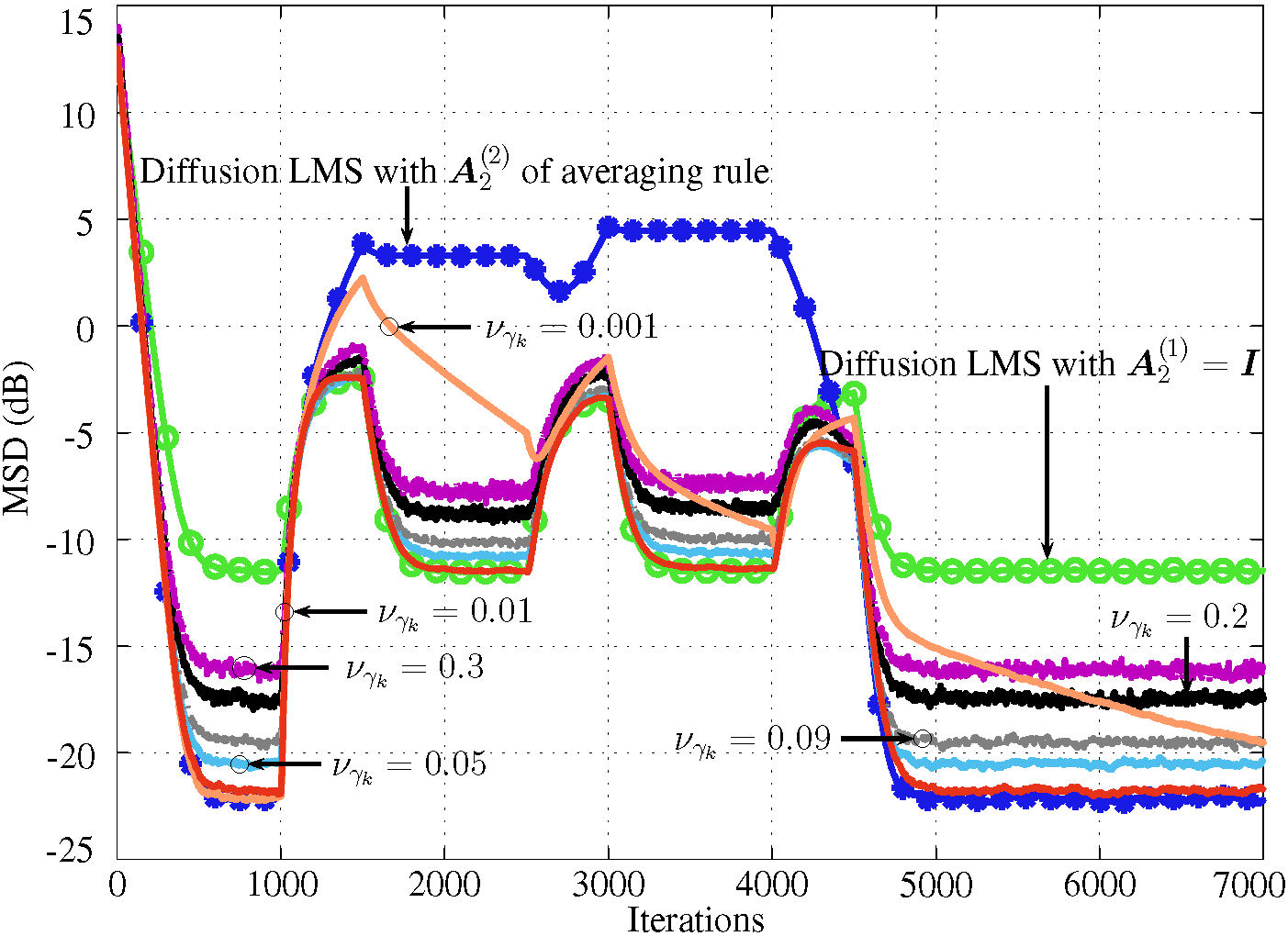
Refer to caption

Fig. 7: Simulation results of the power-normalized scheme with different step-sizes νγk\nu_{\gamma_{k}}.

Refer to caption

Fig. 8: Simulation results of the sign-regressor scheme with different step-sizes νγk\nu_{\gamma_{k}}.

VI-B Theoretical models

To illustrate the theoretical results as well as challenge the assumptions and approximations adopted in the theoretical analysis, we considered three networks with different connectivity parameters as described in Table I. Net1 consisted of 1010 nodes with the network topology given in Fig. 2(a). Net2 was a more complicated network consisting of 2020 nodes. Net3 was generated by dividing 2020 nodes into seven fully connected clusters, with 33 nodes in each of the first six clusters and 22 nodes in the last cluster. These seven clusters were connected in chain, with a single edge connecting adjacent clusters: agent 33 (in cluster 11) was connected with agent 44 (in cluster 22), and agent 66 (in cluster 22) was connected with agent 77 (in cluster 33), and so on until agent 1818 (in cluster 66) was connected to agent 1919 (in cluster 77).

TABLE I: Network statistics for theoretical models validation. 𝐋\bm{L} is the Laplacian matrix associated with the graph (network), λ2​(𝐋)\lambda_{2}(\bm{L}) is the algebraic connectivity [35] of graph, size is the number of nodes, density is the number of non-zero entries of the adjacency matrix of graph, and diameter is the maximum distance between any two nodes [36].
Network Size Density λ2​(𝑳)\lambda_{2}(\bm{L}) Diameter
Net1 10 44% 0.7962 3
Net2 20 38% 0.9549 3
Net3 20 17.25% 0.0439 13

The unknown coefficient vectors to be estimated were of length L=2L=2. We first considered regressors drawn from a zero-mean Gaussian distribution with covariance matrix 𝑹x,k=σx,k2​𝑰L\bm{R}_{x,k}=\sigma_{x,k}^{2}\bm{I}_{L}. Next we considered colored regressors 𝒙k,n=[xk,n​xk,n−1]⊤\bm{x}_{k,n}=[x_{k,n}\,\,x_{k,n-1}]^{\top} generated from a first-order AR model: xk,n=0.5​xk,n−1+0.75​σx,k2​wk,n.x_{k,n}=0.5x_{k,n-1}+\sqrt{0.75\sigma^{2}_{x,k}}w_{k,n}. The input signal wk,nw_{k,n} was i.i.d and drawn from a zero-mean Gaussian distribution, with variance σw2=1\sigma^{2}_{w}=1, so that:

𝑹x,k=σx,k2​(10.50.51).\bm{R}_{x,k}=\sigma^{2}_{x,k}\left(\begin{array}[]{cc}1&0.5\\ 0.5&1\end{array}\right). (89)

Refer to caption

Fig. 9: Illustration of simulation results (model vs. Monte Carlo) for the power-normalized scheme in Net1 and SNR1. Transient and steady-state values of 𝔼​{γk,n}{\mathbb{E}}\{\gamma_{k,n}\} derived in (136) and (95) (top), as well as these of 𝔼​{γk,n2}{\mathbb{E}}\{\gamma_{k,n}^{2}\} derived in (141) and (78) (bottom) for network step-size 0.010.01 (a) and 0.0020.002 (c); (b) Transient and steady-state cross-MSDs derived in (123) and (130).

Refer to caption

Fig. 10: Network performance with the power-normalized scheme (model vs. Monte Carlo) with two different network step-sizes in Net1 and SNR1. For each step-size, the results plotted with a same color stand for same diffusion strategy. For each component diffusion strategy, theoretical transient MSD and theoretical steady-state MSD are derived in (121) and (127). The combination results are derived in (58) and (132).

Refer to caption

Fig. 11: Illustration of simulation results (model vs. Monte Carlo) of the sign-regressor scheme in Net1 and SNR1. Transient and steady-state values of 𝔼​{γk,n}{\mathbb{E}}\{\gamma_{k,n}\} derived in (150) and (95) (top), as well as 𝔼​{γk,n2}{\mathbb{E}}\{\gamma_{k,n}^{2}\} derived in (154) and (78) (bottom) for network step-size 0.010.01 (a) and 0.0020.002 (c); (b) Transient and steady-state cross-MSDs derived in (123) and (130).

The noise signals were generated from Gaussian distributions 𝒩⁡(0,σz,k2){\mathcal{N}}(0,\sigma_{z,k}^{2}). Variances σx,k2\sigma_{x,k}^{2} and σz,k2\sigma_{z,k}^{2} at each agent were generated randomly. By varying σz,k2\sigma_{z,k}^{2}, we changed the signal-to-noise ratio (SNR) [37] to three levels as described in Table II. Both combination schemes were run with network step-sizes being set to {0.01, 0.002}\{0.01,\,0.002\}, and with νγk\nu_{\gamma_{k}} correspondingly being set to {0.01, 0.002}\{0.01,\,0.002\} and {0.015, 0.001}\{0.015,\,0.001\} for power-normalized diffusion and sign-regressor diffusion, respectively. Besides, we set ε\varepsilon to 0.050.05 and η\eta to 0.950.95 for power-normalized diffusion. We first validated the theoretical results related to the mean and mean-square behaviors of γk,n\gamma_{k,n}, the theoretical MSD of each component strategy, as well as cross-MSD of the whole network defined by MSDcross≜1N​𝔼​{𝒗n(1)⊤​𝒗n(2)}{\rm MSD}_{\rm cross}\triangleq\frac{1}{N}{\mathbb{E}}\bigl\{\bm{v}_{n}^{(1)\top}\bm{v}_{n}^{(2)}\bigr\}. Then we evaluated the theoretical MSD behavior of the combined strategy.

TABLE II: Three SNR levels in decibel (dB) for theoretical models validation. Since SNRs vary from node to node, we enumerate the Maximum, Minimum and Mean values.
SNR Level Maximum Minimum Mean
SNR1 3.5724 1.6673 2.7946
SNR2 -9.4379 -11.343 -10.2157
SNR3 -18.9803 -20.8855 -19.7581

The results for white Gaussian inputs with Net1 and SNR1 are plotted in Fig. 9–Fig. 12. In both Fig. 9 and Fig. 11, we observe that the simulated transient values and theoretical transient values accurately matched, especially for small step-sizes, since the approximations adopted in theoretical analyses are more reasonable for small step-sizes. Further, we observe that a larger νγk\nu_{\gamma_{k}} results in a faster convergence rate, which coincidences with equations (138) and (151) in theoretical analyses. In Fig. 10 and Fig. 12, besides the accurate matching of the simulated and theoretical MSD learning curves, the almost superposition of theoretical steady-state MSDs for combined strategy and that of the best component validates the conclusion again that the combination schemes are universal at steady state. Further, the gaps of these two theoretical values becomes smaller as the step-sizes decrease, since the analyses of the universality are based on the approximations that are more valid for small step-sizes.

The results of the power-normalized diffusion for white Gaussian inputs with Net2 and Net3 in SNR1 are plotted in Fig. 13 and Fig. 14, respectively. And the results with Net1 in SNR2 and SNR3 are plotted in Fig. 15 and Fig. 16, respectively. Together with Fig. 10, all these validate the accuracy of theoretical analyses under different SNR conditions and network connectivity parameters.

The results of the power-normalized diffusion for correlated input with Net1 and SNR1 are plotted in Fig. 17. Though assumption A2 is violated, the superimposition of simulated and theoretical curves validates the accuracy of the theoretical analyses for sufficiently small step-sizes with moderately correlated regressors.

Refer to caption

Fig. 12: Network performance with the sign-regressor scheme in Net1 and SNR1.

Refer to caption

Fig. 13: Network performance with the power-normalized scheme in Net2 and SNR1, and the network step-sizes are 0.010.01.

Refer to caption

Fig. 14: Network performance with the power-normalized scheme in Net3 and SNR1, and the network step-sizes are 0.010.01

.

Refer to caption

Fig. 15: Network performance with the power-normalized scheme in Net1 and SNR2, and the network step-sizes are 0.010.01.

Refer to caption

Fig. 16: Network performance with the power-normalized scheme in Net1 and SNR3, and the network step-sizes are 0.010.01.

Refer to caption

Fig. 17: Network performance with the power-normalized scheme using correlated inputs in Net1 and SNR1.

VII CONCLUSION AND PERSPECTIVES

Combining diffusion strategies enables a network to reach better performance. In this paper, we proposed two schemes for affine combination of two diffusion strategies. By using the proposed combination schemes, we obtained a combined diffusion strategy ensuring the advantages of both component strategies simultaneously, sometimes even better, in terms of EMSE. We conducted theoretical analyses in the mean and mean-square sense, and analyzed the universality of each approach. Simulation results illustrate the interesting properties of affine combination schemes, as well as the accuracy of the theoretical results. Several open problems still have to be addressed. For instance, it would be interesting to design combination schemes and conduct theoretical analysis for colored measurement noise and correlated regressors. Some works focusing on adaptive networks with colored measurement noise include [38, 39, 40]. It would also be interesting to explore other combination frameworks and schemes.

Appendix A
Combination Scheme for Multiple Strategies

The general scheme follows the description from Section III except that we now have MM component diffusion strategies. We introduce MM affine combination coefficients γk,n(1),γk,n(2),⋯,γk,n(M)\gamma_{k,n}^{(1)},\gamma_{k,n}^{(2)},\cdots,\gamma_{k,n}^{(M)} for node kk at time instant nn, satisfying the constraint ∑i=1Mγk,n(i)=1\sum_{i=1}^{M}\gamma_{k,n}^{(i)}=1. By combining the estimates of MM component strategies at each agent kk, we obtain the overall system coefficients 𝒘k,n\bm{w}_{k,n} and estimation error ek,ne_{k,n} at combination layer, with ek,n=∑i=1Mγk,n(i)​ek,n(i)e_{k,n}=\sum_{i=1}^{M}\gamma_{k,n}^{(i)}e_{k,n}^{(i)}. In order to keep γk,n(i)\gamma_{k,n}^{(i)} satisfying the sum-to-one constraint, we calculate γk,n(i)\gamma_{k,n}^{(i)} via the mapping:

γk,n(i)=αk,n(i)+δ∑j=1Mαk,n(j)+M​δ,\gamma_{k,n}^{(i)}=\frac{\alpha_{k,n}^{(i)}+\delta}{\sum_{j=1}^{M}\alpha_{k,n}^{(j)}+M\delta},\vskip-5.69054pt (90)

where αk,n(i)\alpha_{k,n}^{(i)} are newly introduced auxiliary parameters, and δ\delta is a small positive constant to avoid zero-division. We shall update αk,n(i)\alpha_{k,n}^{(i)} instead of updating γk,n(i)\gamma_{k,n}^{(i)} directly. By minimizing the MSE (16) over the entire network, and using stochastic gradient approximation, we obtain:

αk,n+1(i)\displaystyle{\alpha}_{k,n+1}^{(i)} ≈αk,n(i)+ναk​ek,n​sgn​{ek,n−ek,n(i)∑j=1Mαk,n(j)+M​δ}.\displaystyle\approx{\alpha}_{k,n}^{(i)}+\nu_{\alpha_{k}}e_{k,n}\text{sgn}\biggl\{\frac{e_{k,n}-e_{k,n}^{(i)}}{\sum_{j=1}^{M}\alpha_{k,n}^{(j)}+M\delta}\biggr\}. (91)

Appendix B
Proof of Universality Analysis Result 1

Starting from the update equation of γk,n\gamma_{k,n} in (20), we know that the stationary point of γk,n\gamma_{k,n} is reached for:

𝔼{νγkε+pk,nek,n𝒙k,n⊤(𝒘k,n(1)−𝒘k,n(2))}=0.\displaystyle{\mathbb{E}}\Bigl\{{\nu_{\gamma_{k}}\over\varepsilon+p_{k,n}}\,e_{k,n}\,\bm{x}_{k,n}^{\top}\bigl({\bm{w}}_{k,n}^{(1)}-{\bm{w}}_{k,n}^{(2)}\bigl)\Bigr\}=0. (92)

Using (27) and (28), we obtain:

𝔼{νγkε+pk,nγk,n[e~k,n(1)e~k,n(2)−(e~k,n(1))2]+\displaystyle{\mathbb{E}}\Bigl\{{\nu_{\gamma_{k}}\over\varepsilon+p_{k,n}}\,\gamma_{k,n}\,\bigl[\widetilde{e}_{k,n}^{(1)}\widetilde{e}_{k,n}^{(2)}-{(\widetilde{e}_{k,n}^{(1)})}^{2}\bigr]+
νγkε+pk,n(1−γk,n)[(e~k,n(2))2−e~k,n(1)e~k,n(2)]}=0,\displaystyle{\nu_{\gamma_{k}}\over\varepsilon+p_{k,n}}\,{\bigl(1-\gamma_{k,n}\bigl)}\,\bigl[{(\widetilde{e}_{k,n}^{(2)})}^{2}-\widetilde{e}_{k,n}^{(1)}\widetilde{e}_{k,n}^{(2)}\bigr]\Bigr\}=0, (93)

where we used the zero-mean property of zk,nz_{k,n} under assumption A1. Though we cannot obtain a closed-form solution for 𝔼​{γk,n}{\mathbb{E}}\{\gamma_{k,n}\} at each time instant, by resorting to approximations Ap1, Ap2 and introducing the quantity △​Jk,n(i)≜Jex,k,n(i)−Jex,k,n(1,2)\triangle J_{k,n}^{(i)}\triangleq J_{\text{ex},k,n}^{(i)}-J_{\text{ex},k,n}^{(1,2)}, with Jex,k,n(1,2)J_{\text{ex},k,n}^{(1,2)} denoting the cross-EMSE defined by Jex,k,n(1,2)≜𝔼⁡{e~k,n(1)​e~k,n(2)}J_{\text{ex},k,n}^{(1,2)}\triangleq{\mathbb{E}}\{\widetilde{e}_{k,n}^{(1)}\widetilde{e}_{k,n}^{(2)}\}, equation (93) at steady-state becomes:

−γ¯k,∞△Jk,∞(1)+(1−γ¯k,∞)△Jk,∞(2)=0\displaystyle-\bar{\gamma}_{k,\infty}\,\triangle J_{k,\infty}^{(1)}+{\bigl(1-\bar{\gamma}_{k,\infty}\bigl)}\,\triangle J_{k,\infty}^{(2)}=0 (94)

with γ¯k,∞≜𝔼⁡{γk,∞}\bar{\gamma}_{k,\infty}\triangleq{\mathbb{E}}\{\gamma_{k,\infty}\}. This leads to a closed-form expression for the stationary point at steady-state:

γ¯k,∞=△​Jk,∞(2)△​Jk,∞(1)+△​Jk,∞(2).\displaystyle\bar{\gamma}_{k,\infty}=\frac{\triangle J_{k,\infty}^{(2)}}{\triangle J_{k,\infty}^{(1)}+\triangle J_{k,\infty}^{(2)}}. (95)

We can now establish the universality of the power-normalized scheme (20) at steady-state by using (95). Under approximation Ap1, and assuming further that the variance of γk,∞\gamma_{k,\infty} is small enough so that the approximation 𝔼⁡{γk,∞2}≈γ¯k,∞2{\mathbb{E}}\{\gamma_{k,\infty}^{2}\}\approx\bar{\gamma}_{k,\infty}^{2} holds, the EMSE at node kk after combination at steady-state can be written as:

Jex,k,∞\displaystyle J_{\text{ex},k,\infty} ≈γ¯k,∞2​Jex,k,∞(1)+(1−γ¯k,∞)2​Jex,k,∞(2)\displaystyle\approx\bar{\gamma}_{k,\infty}^{2}\,J_{\text{ex},k,\infty}^{(1)}+{(1-\bar{\gamma}_{k,\infty})}^{2}\,J_{\text{ex},k,\infty}^{(2)}
+2​γ¯k,∞​(1−γ¯k,∞)​Jex,k,∞(1,2).\displaystyle\quad+2\bar{\gamma}_{k,\infty}{(1-\bar{\gamma}_{k,\infty})}\,J_{\text{ex},k,\infty}^{(1,2)}. (96)

By substituting γ¯k,∞\bar{\gamma}_{k,\infty} in (95) into (96), and after some algebraic manipulations, we arrive at:

Jex,k,∞=Jex,k,∞(1,2)+△​Jk,∞(1)​△​Jk,∞(2)△​Jk,∞(1)+△​Jk,∞(2).\displaystyle J_{\text{ex},k,\infty}=J_{\text{ex},k,\infty}^{(1,2)}+\frac{\triangle J_{k,\infty}^{(1)}\triangle J_{k,\infty}^{(2)}}{\triangle J_{k,\infty}^{(1)}+\triangle J_{k,\infty}^{(2)}}. (97)

From Cauchy-Schwartz inequality, we know that Jex,k,∞(1,2)J_{\text{ex},k,\infty}^{(1,2)} cannot be simultaneously larger than Jex,k,∞(1)J_{\text{ex},k,\infty}^{(1)} and Jex,k,∞(2)J_{\text{ex},k,\infty}^{(2)}. Therefore, to evaluate (97), we split the problem into three cases according to the relations between Jex,k,∞(1,2)J_{\text{ex},k,\infty}^{(1,2)} and Jex,k,∞(i)J_{\text{ex},k,\infty}^{(i)}:

  • •

    Case 1: Jex,k,∞(i)≥Jex,k,∞(1,2)J_{\text{ex},k,\infty}^{(i)}\geq J_{\text{ex},k,\infty}^{(1,2)} for i=1,2i=1,2, which means △​Jk,∞(1)≥0\triangle J_{k,\infty}^{(1)}\geq 0 and △​Jk,∞(2)≥0\triangle J_{k,\infty}^{(2)}\geq 0 at the same time. Since △​Jk,∞(1)​△​Jk,∞(2)△​Jk,∞(1)+△​Jk,∞(2)≤△​Jk,∞(1)\frac{\triangle J_{k,\infty}^{(1)}\triangle J_{k,\infty}^{(2)}}{\triangle J_{k,\infty}^{(1)}+\triangle J_{k,\infty}^{(2)}}\leq\triangle J_{k,\infty}^{(1)} and △​Jk,∞(1)​△​Jk,∞(2)△​Jk,∞(1)+△​Jk,∞(2)≤△​Jk,∞(2)\frac{\triangle J_{k,\infty}^{(1)}\triangle J_{k,\infty}^{(2)}}{\triangle J_{k,\infty}^{(1)}+\triangle J_{k,\infty}^{(2)}}\leq\triangle J_{k,\infty}^{(2)}, we conclude from (97) that:

    Jex,k,∞≤Jex,k,∞(1)andJex,k,∞≤Jex,k,∞(2).\displaystyle J_{\text{ex},k,\infty}\leq J_{\text{ex},k,\infty}^{(1)}\quad\text{and}\quad J_{\text{ex},k,\infty}\leq J_{\text{ex},k,\infty}^{(2)}. (98)
  • •

    Case 2: Jex,k,∞(1)<Jex,k,∞(1,2)<Jex,k,∞(2)J_{\text{ex},k,\infty}^{(1)}<J_{\text{ex},k,\infty}^{(1,2)}<J_{\text{ex},k,\infty}^{(2)}, which corresponds to △​Jk,∞(1)<0\triangle J_{k,\infty}^{(1)}<0 and △​Jk,∞(2)>0\triangle J_{k,\infty}^{(2)}>0. Then (97) leads to:

    Jex,k,∞=Jex,k,∞(1)−(△​Jk,∞(1))2△​Jk,∞(1)+△​Jk,∞(2).\displaystyle J_{\text{ex},k,\infty}=J_{\text{ex},k,\infty}^{(1)}-\frac{{\bigl(\triangle J_{k,\infty}^{(1)}\bigr)}^{2}}{\triangle J_{k,\infty}^{(1)}+\triangle J_{k,\infty}^{(2)}}.\vskip-5.69054pt (99)

    Since △​Jk,∞(1)+△​Jk,∞(2)>0{\triangle J_{k,\infty}^{(1)}+\triangle J_{k,\infty}^{(2)}}>0, we have Jex,k,∞<Jex,k,∞(1)J_{\text{ex},k,\infty}<J_{\text{ex},k,\infty}^{(1)}. As a result, Jex,k,∞<min⁡{Jex,k,∞(1),Jex,k,∞(2)}J_{\text{ex},k,\infty}<\min\,\bigl\{J_{\text{ex},k,\infty}^{(1)},J_{\text{ex},k,\infty}^{(2)}\bigr\}.

  • •

    Case 3: Jex,k,∞(1)>Jex,k,∞(1,2)>Jex,k,∞(2)J_{\text{ex},k,\infty}^{(1)}>J_{\text{ex},k,\infty}^{(1,2)}>J_{\text{ex},k,\infty}^{(2)}. Due to the symmetry of (97) for △​Jk,∞(1)\triangle J_{k,\infty}^{(1)} and △​Jk,∞(2)\triangle J_{k,\infty}^{(2)}, we obtain the same conclusion as Case 2.

Therefore, at steady-state when the combination coefficient (95) is applied, the resulting EMSE after combination cannot be worse than that of the best component, that is,

Jex,k,∞≤min⁡{Jex,k,∞(1),Jex,k,∞(2)}.\displaystyle J_{\text{ex},k,\infty}\leq\min\,\bigl\{J_{\text{ex},k,\infty}^{(1)},J_{\text{ex},k,\infty}^{(2)}\bigr\}. (100)

We also conclude that equation (29) holds. It means that the EMSE of the diffusion network after combination cannot be worse than that of the best component strategies, leading to the universality property of the power-normalized scheme at steady state.

Appendix C
Proof of Stability Analysis Result 1

𝔼​{𝒗n+1}{\mathbb{E}}\bigl\{\bm{v}_{n+1}\bigr\} converges as n→∞n\to\infty if, and only if, both terms on the right-hand side (RHS) of (40) converge to finite values. Using (42) and iterating the first term from 𝔼​{𝒗0(1)}{\mathbb{E}}\bigl\{\bm{v}^{(1)}_{0}\bigr\}, we obtain:

𝔼⁡{𝚪n+1}​𝔼​{𝒗n+1(1)}\displaystyle{\mathbb{E}}\bigl\{\bm{\Gamma}_{n+1}\bigr\}\,{\mathbb{E}}\bigl\{\bm{v}_{n+1}^{(1)}\bigr\} =𝔼⁡{𝚪n+1}​(𝑩¯(1))n+1​𝔼​{𝒗0(1)}\displaystyle={\mathbb{E}}\bigl\{\bm{\Gamma}_{n+1}\bigr\}{\bigl(\overline{\bm{B}}^{(1)}\bigr)}^{n+1}{\mathbb{E}}\bigl\{\bm{v}^{(1)}_{0}\bigr\}
−∑j=0n𝔼{𝚪n+1}(𝑩¯(1))j𝒓¯(1).\displaystyle\quad-\sum_{j=0}^{n}{\mathbb{E}}\bigl\{\bm{\Gamma}_{n+1}\bigr\}{\bigl(\overline{\bm{B}}^{(1)}\bigr)}^{j}\overline{\bm{r}}^{(1)}. (101)

To prove convergence of (101), it is sufficient to prove that the sequence s1,m≜[𝔼⁡{𝚪n+1}​(𝑩¯(1))n+1​𝔼​{𝒗0(1)}]ms_{1,m}\triangleq\Bigl[{\mathbb{E}}\bigl\{\bm{\Gamma}_{n+1}\bigr\}{\bigl(\overline{\bm{B}}^{(1)}\bigr)}^{n+1}{\mathbb{E}}\bigl\{\bm{v}^{(1)}_{0}\bigr\}\Bigr]_{m} and series ∑j=0n[𝔼⁡{𝚪n+1}​(𝑩¯(1))j​𝒓¯(1)]m\sum_{j=0}^{n}\Bigl[{\mathbb{E}}\bigl\{\bm{\Gamma}_{n+1}\bigr\}{\bigl(\overline{\bm{B}}^{(1)}\bigr)}^{j}\overline{\bm{r}}^{(1)}\Bigr]_{m} converge for m=1,⋯,N​Lm=1,\cdots,NL. It is known that a sequence is convergent if it is upper bounded and lower bounded by two sequences with the same limit [41]. A series is absolutely convergent if each of its terms is bounded by a term of an absolutely convergent series [42, 43]. Define s2,m≜[𝔼⁡{𝚪n+1}​(𝑩¯(1))j​𝒓¯(1)]ms_{2,m}\triangleq\Bigl[{\mathbb{E}}\bigl\{\bm{\Gamma}_{n+1}\bigr\}{\bigl(\overline{\bm{B}}^{(1)}\bigr)}^{j}\overline{\bm{r}}^{(1)}\Bigr]_{m}. Since the largest absolute value of the entries in a block vector is smaller than or equal to the block maximum norm of this vector, we have:

|s1,m|\displaystyle|s_{1,m}| ≤‖𝔼⁡{𝚪n+1}‖b,∞⋅‖𝑩¯(1)‖b,∞n+1⋅‖𝔼⁡{𝒗0(1)}‖b,∞\displaystyle\!\leq\bigl\|{\mathbb{E}}\bigl\{\bm{\Gamma}_{n+1}\bigr\}\bigr\|_{b,\infty}\cdot\bigl\|\overline{\bm{B}}^{(1)}\bigr\|_{b,\infty}^{n+1}\cdot\bigl\|{\mathbb{E}}\bigl\{\bm{v}^{(1)}_{0}\bigr\}\bigr\|_{b,\infty}
≤(44)​‖𝔼⁡{𝚪n+1}‖b,∞⋅‖𝑴(1)‖b,∞n+1⋅‖𝔼⁡{𝒗0(1)}‖b,∞\displaystyle\!\overset{\eqref{eq:Bi}}{\leq}\bigl\|{\mathbb{E}}\bigl\{\bm{\Gamma}_{n+1}\bigr\}\bigr\|_{b,\infty}\cdot\bigl\|\bm{M}^{(1)}\bigr\|_{b,\infty}^{n+1}\cdot\bigl\|{\mathbb{E}}\bigl\{\bm{v}^{(1)}_{0}\bigr\}\bigr\|_{b,\infty}
=ρ⁡(𝔼⁡{𝚪n+1})⋅[ρ⁡(𝑴(1))]n+1​‖𝔼⁡{𝒗0(1)}‖b,∞,\displaystyle\!=\!\rho\bigl({\mathbb{E}}\bigl\{\bm{\Gamma}_{n+1}\bigr\}\bigr)\!\cdot\!\bigl[\rho\bigl(\bm{M}^{(1)}\bigr)\bigr]^{n+1}\,\bigl\|{\mathbb{E}}\bigl\{\bm{v}^{(1)}_{0}\bigr\}\bigr\|_{b,\infty}, (102)
|s2,m|\displaystyle|s_{2,m}| ≤‖𝔼⁡{𝚪n+1}‖b,∞⋅‖𝑩¯(1)‖b,∞j⋅‖𝒓¯(1)‖b,∞\displaystyle\leq\bigl\|{\mathbb{E}}\bigl\{\bm{\Gamma}_{n+1}\bigr\}\bigr\|_{b,\infty}\cdot\bigl\|\overline{\bm{B}}^{(1)}\bigr\|_{b,\infty}^{j}\cdot\bigl\|\overline{\bm{r}}^{(1)}\bigr\|_{b,\infty}
≤(44)​ρ​(𝔼⁡{𝚪n+1})⋅[ρ⁡(𝑴(1))]j⋅‖𝒓¯(1)‖b,∞,\displaystyle\overset{\eqref{eq:Bi}}{\leq}\rho\bigl({\mathbb{E}}\bigl\{\bm{\Gamma}_{n+1}\bigr\}\bigr)\cdot\bigl[\rho\bigl(\bm{M}^{(1)}\bigr)\bigr]^{j}\cdot\bigl\|\overline{\bm{r}}^{(1)}\bigr\|_{b,\infty}, (103)

where

𝑴(1)≜𝑰N​L−𝑼(1)​𝑯¯(1),\displaystyle\bm{M}^{(1)}\triangleq\bm{I}_{NL}-\bm{U}^{(1)}\overline{\bm{H}}^{(1)}, (104)

∥⋅∥b,∞\|\cdot\|_{b,\infty} is the block maximum norm [5], and ρ⁡(⋅)\rho(\cdot) is the spectral radius of a given matrix. Since 𝔼​{𝒗0(1)}{\mathbb{E}}\bigl\{\bm{v}^{(1)}_{0}\bigr\} and 𝒓¯(1)\overline{\bm{r}}^{(1)} are bounded, it is sufficient to require that ρ⁡(𝑴(1))<1\rho\bigl(\bm{M}^{(1)}\bigr)<1 and ρ⁡(𝔼​{𝚪n+1})\rho\bigl({\mathbb{E}}\bigl\{\bm{\Gamma}_{n+1}\bigr\}\bigr) is uniformly bounded. It is similar for the second term on the RHS of (40). As discussed later in Section IV-C, condition (56) ensures the convergence of 𝔼​{𝚪n+1}{\mathbb{E}}\bigl\{\bm{\Gamma}_{n+1}\bigr\} and 𝔼⁡{𝑰N​L−𝚪n+1}{\mathbb{E}}\bigl\{\bm{I}_{NL}-\bm{\Gamma}_{n+1}\bigr\}. Given that νγk\nu_{\gamma_{k}} satisfies condition (56), the convergence of (40) requires only ρ⁡(𝑰N​L−𝑼(i)​𝑯¯(i))<1\rho\bigl(\bm{I}_{NL}-\bm{U}^{(i)}\overline{\bm{H}}^{(i)}\bigr)<1, which is ensured by step-sizes satisfying (55).

For the asymptotic bias, from (40) and (42), we obtain:

𝔼​{𝒗∞}\displaystyle\hskip-5.69054pt{\mathbb{E}}\bigl\{\bm{v}_{\infty}\bigr\} =𝔼⁡{𝚪∞}​𝔼​{𝒗∞(1)}+(𝑰N​L−𝔼⁡{𝚪∞})​𝔼​{𝒗∞(2)}\displaystyle\!\!=\!{\mathbb{E}}\bigl\{\bm{\Gamma}_{\infty}\bigr\}{\mathbb{E}}\bigl\{\bm{v}_{\infty}^{(1)}\bigr\}\!+\!(\bm{I}_{NL}\!-\!{\mathbb{E}}\bigl\{\bm{\Gamma}_{\infty}\bigr\})\,{\mathbb{E}}\bigl\{\bm{v}_{\infty}^{(2)}\bigr\} (105)
𝔼​{𝒗∞(i)}\displaystyle\hskip-5.69054pt{\mathbb{E}}\bigl\{\bm{v}_{\infty}^{(i)}\bigr\} =−(𝑰N​L−𝑩¯(i))−1​𝒓¯(i),\displaystyle\!=\!-{\bigl(\bm{I}_{NL}-\overline{\bm{B}}^{(i)}\bigr)}^{-1}\overline{\bm{r}}^{(i)}, (106)

which leads to expression (57).

Appendix D
Derivation of Equation (62)

Using (41), (63), (65), and approximation Ap4, we have:

𝔼⁡{‖𝒗n+1(i)‖𝚺n+1(i)2}\displaystyle{\mathbb{E}}\Bigl\{{\bigl\|\bm{v}_{n+1}^{(i)}\bigr\|}^{2}_{\bm{\Sigma}^{(i)}_{n+1}}\Bigr\} =𝔼⁡{‖𝒗n(i)‖𝚺B,n+1(i)2}+trace​{𝚺n+1(i)​𝑮(i)}\displaystyle={\mathbb{E}}\Bigl\{{\bigl\|\bm{v}_{n}^{(i)}\bigr\|}^{2}_{\bm{\Sigma}^{(i)}_{B,n+1}}\Bigr\}+\text{trace}\Bigl\{\bm{\Sigma}^{(i)}_{n+1}\,\bm{G}^{(i)}\Bigr\}
+𝔼⁡{𝒇⁡(𝒓n(i),𝚺n+1(i),𝒗n(i))}\displaystyle\quad+{\mathbb{E}}\bigl\{\bm{f}(\bm{r}_{n}^{(i)},\bm{\Sigma}^{(i)}_{n+1},\bm{v}_{n}^{(i)})\bigr\} (107)

with

𝚺B,n+1(i)\displaystyle\hskip-8.53581pt\bm{\Sigma}^{(i)}_{B,n+1} ≜𝔼⁡{𝑩n(i)⊤​𝚺n+1(i)​𝑩n(i)}.\displaystyle\triangleq{\mathbb{E}}\bigl\{\bm{B}_{n}^{(i)\top}\bm{\Sigma}^{(i)}_{n+1}\bm{B}_{n}^{(i)}\bigr\}. (108)

In the derivation of expression (107), we used relation 𝔼⁡{𝒈n(i)}=0{\mathbb{E}}\{\bm{g}_{n}^{(i)}\}=0, which is derived from (50) and (51) directly by using the zero-mean property of zℓ,nz_{\ell,n}.

Let 𝝈B,n+1(i)=vec​{𝚺B,n+1(i)}\bm{\sigma}_{B,n+1}^{(i)}=\text{vec}\bigl\{\bm{\Sigma}_{B,n+1}^{(i)}\bigr\}. Under approximation Ap4, and using the properties of vec​{⋅}\text{vec}\{\cdot\} operator, we have:

𝝈B,n+1(i)=𝑲(i)​𝝈n+1(i),\displaystyle\bm{\sigma}_{B,n+1}^{(i)}=\bm{K}^{(i)}\,\bm{\sigma}^{(i)}_{n+1}, (109)

where

𝑲(i)\displaystyle\bm{K}^{(i)} ≜𝔼⁡{𝑩n(i)⊤⊗𝑩n(i)⊤}≈𝑩¯(i)⊤⊗𝑩¯(i)⊤\displaystyle\triangleq{\mathbb{E}}\bigl\{\bm{B}_{n}^{(i)\top}\otimes\bm{B}_{n}^{(i)\top}\bigr\}\approx\overline{\bm{B}}^{(i)\top}\otimes\overline{\bm{B}}^{(i)\top} (110)

for sufficiently small step-sizes. We have:

trace​{𝚺n+1(i)​𝑮(i)}=[vec​{𝑮(i)⊤}]⊤​𝝈n+1(i).\text{trace}\bigl\{\bm{\Sigma}^{(i)}_{n+1}\,\bm{G}^{(i)}\bigr\}={\bigl[\text{vec}\{\bm{G}^{(i)\top}\}\bigr]}^{\top}\bm{\sigma}^{(i)}_{n+1}. (111)

For sufficiently small step-sizes, we have:

𝔼⁡{𝒇⁡(𝒓n(i),𝚺n+1(i),𝒗n(i))}\displaystyle{\mathbb{E}}\bigl\{\bm{f}(\bm{r}_{n}^{(i)},\bm{\Sigma}^{(i)}_{n+1},\bm{v}_{n}^{(i)})\bigr\} ≈𝒇⁡(𝒓¯(i),𝚺n+1(i),𝔼⁡{𝒗n(i)}).\displaystyle\approx\bm{f}\bigl(\overline{\bm{r}}^{(i)},\bm{\Sigma}^{(i)}_{n+1},{\mathbb{E}}\bigl\{\bm{v}_{n}^{(i)}\bigr\}\bigr). (112)

Substituting (111) and (112) into (107) yields expression (62).

Appendix E
Proof of Stability Analysis Result 2

The convergence of 𝔼⁡{‖𝒗n+1‖𝚺2}{\mathbb{E}}\bigl\{{\|\bm{v}_{n+1}\|}^{2}_{\bm{\Sigma}}\bigr\} requires the convergence of the terms on the RHS of (58). For the last term, using (62) and iterating from n=0n=0, we find that

𝔼⁡{‖𝒗n+1(1)‖𝝈n+1(1)2}=‖𝒗0(1)‖(𝑲(1))n+1​𝝈n+1(1)2\displaystyle{\mathbb{E}}\bigl\{\bigl\|\bm{v}_{n+1}^{(1)}\bigr\|^{2}_{\bm{\sigma}^{(1)}_{n+1}}\bigr\}=\bigl\|\bm{v}_{0}^{(1)}\bigr\|^{2}_{{(\bm{K}^{(1)})}^{n+1}\bm{\sigma}^{(1)}_{n+1}}
+[vec{𝑮(1)⊤}]⊤∑t=0n(𝑲(1))t𝝈n+1(1)\displaystyle+{\bigl[\text{vec}\{\bm{G}^{(1)\top}\}\bigr]}^{\top}\sum_{t=0}^{n}{(\bm{K}^{(1)})}^{t}\bm{\sigma}^{(1)}_{n+1}
+∑t=0n𝒇(𝒓¯(1),(𝑲(1))t𝝈n+1(1),𝔼{𝒗n−t(1)})\displaystyle+\sum_{t=0}^{n}\bm{f}\bigl(\overline{\bm{r}}^{(1)},{(\bm{K}^{(1)})}^{t}\bm{\sigma}^{(1)}_{n+1},{\mathbb{E}}\bigl\{\bm{v}_{n-t}^{(1)}\bigr\}\bigr) (113)

for n≥0n\geq 0 with initial condition 𝒗0(1)=𝒘0(1)−𝒘⋆\bm{v}_{0}^{(1)}=\bm{w}_{0}^{(1)}-\bm{w}^{\star}. Since

𝝈n+1(1)=𝔼⁡{𝚪n+1⊤⊗𝚪n+1⊤}​𝝈\displaystyle\bm{\sigma}^{(1)}_{n+1}={\mathbb{E}}\bigl\{\bm{\Gamma}_{n+1}^{\top}\otimes\bm{\Gamma}_{n+1}^{\top}\bigr\}\bm{\sigma} (114)

where 𝝈≜vec​{𝚺}\bm{\sigma}\triangleq\text{vec}\{\bm{\Sigma}\}, the convergence of (113) requires that the sequence s3,m≜[(𝑲(1))n+1​𝔼​{𝚪n+1⊤⊗𝚪n+1⊤}​𝝈]ms_{3,m}\triangleq\bigl[{(\bm{K}^{(1)})}^{n+1}\,{\mathbb{E}}\bigl\{\bm{\Gamma}_{n+1}^{\top}\otimes\bm{\Gamma}_{n+1}^{\top}\bigr\}\bm{\sigma}\bigr]_{m} and series ∑t=0n[(𝑲(1))t​𝔼​{𝚪n+1⊤⊗𝚪n+1⊤}​𝝈]m\sum_{t=0}^{n}\bigl[{(\bm{K}^{(1)})}^{t}{\mathbb{E}}\bigl\{\bm{\Gamma}_{n+1}^{\top}\otimes\bm{\Gamma}_{n+1}^{\top}\bigr\}\bm{\sigma}\bigr]_{m} be convergent for m=1,⋯,(N​L)2m=1,\cdots,{(NL)}^{2}. Define s4,m≜[(𝑲(1))t​𝔼​{𝚪n+1⊤⊗𝚪n+1⊤}​𝝈]ms_{4,m}\triangleq\bigl[{(\bm{K}^{(1)})}^{t}{\mathbb{E}}\bigl\{\bm{\Gamma}_{n+1}^{\top}\otimes\bm{\Gamma}_{n+1}^{\top}\bigr\}\bm{\sigma}\bigr]_{m}. Similar to (102) and (103), we have:

|s3,m|\displaystyle|s_{3,m}| ≤‖𝑲(1)‖b,∞n+1⋅‖𝔼⁡{𝚪n+1⊤⊗𝚪n+1⊤}‖b,∞​‖𝝈‖b,∞\displaystyle\leq\bigl\|\bm{K}^{(1)}\bigr\|_{b,\infty}^{n+1}\cdot\bigl\|{\mathbb{E}}\bigl\{\bm{\Gamma}_{n+1}^{\top}\otimes\bm{\Gamma}_{n+1}^{\top}\bigr\}\bigr\|_{b,\infty}\bigl\|\bm{\sigma}\bigr\|_{b,\infty}
=‖𝑲(1)‖b,∞n+1⋅ρ⁡(𝔼⁡{𝚪n+1⊤⊗𝚪n+1⊤})​‖𝝈‖b,∞,\displaystyle=\bigl\|\bm{K}^{(1)}\bigr\|_{b,\infty}^{n+1}\cdot\rho\bigl({\mathbb{E}}\bigl\{\bm{\Gamma}_{n+1}^{\top}\otimes\bm{\Gamma}_{n+1}^{\top}\bigr\}\bigr)\bigl\|\bm{\sigma}\bigr\|_{b,\infty}, (115)
|s4,m|\displaystyle|s_{4,m}| ≤‖𝑲(1)‖b,∞t⋅‖𝔼⁡{𝚪n+1⊤⊗𝚪n+1⊤}‖b,∞​‖𝝈‖b,∞\displaystyle\leq\bigl\|\bm{K}^{(1)}\bigr\|_{b,\infty}^{t}\cdot\bigl\|{\mathbb{E}}\bigl\{\bm{\Gamma}_{n+1}^{\top}\otimes\bm{\Gamma}_{n+1}^{\top}\bigr\}\bigr\|_{b,\infty}\bigl\|\bm{\sigma}\bigr\|_{b,\infty}
=‖𝑲(1)‖b,∞t⋅ρ⁡(𝔼⁡{𝚪n+1⊤⊗𝚪n+1⊤})⋅‖𝝈‖b,∞.\displaystyle\!=\!\bigl\|\bm{K}^{(1)}\bigr\|_{b,\infty}^{t}\!\cdot\rho\bigl({\mathbb{E}}\bigl\{\bm{\Gamma}_{n+1}^{\top}\otimes\bm{\Gamma}_{n+1}^{\top}\bigr\}\bigr)\cdot\bigl\|\bm{\sigma}\bigr\|_{b,\infty}. (116)

According to assumption A2, we have:

𝔼⁡{γk,n+1​γℓ,n+1}=0,∀k≠ℓ.\displaystyle{\mathbb{E}}\{\gamma_{k,n+1}\gamma_{\ell,n+1}\}=0,\,\forall k\neq\ell. (117)

Thus, ρ⁡(𝔼⁡{𝚪n+1⊤⊗𝚪n+1⊤})\rho\bigl({\mathbb{E}}\bigl\{\bm{\Gamma}_{n+1}^{\top}\otimes\bm{\Gamma}_{n+1}^{\top}\bigr\}\bigr) is bounded as long as 𝔼​{𝚪n+1​𝚪n+1}{\mathbb{E}}\{{\bm{\Gamma}_{n+1}\bm{\Gamma}_{n+1}}\} is convergent. We further have:

‖𝑲(1)‖b,∞\displaystyle\bigl\|\bm{K}^{(1)}\bigr\|_{b,\infty} =(64)​‖𝑩¯(1)⊤⊗𝑩¯(1)⊤‖b,∞\displaystyle\overset{\eqref{eq:ApproxKi}}{=}{\bigl\|\overline{\bm{B}}^{(1)\top}\otimes\overline{\bm{B}}^{(1)\top}\bigr\|}_{b,\infty}
≤(44)​‖𝒜1(1)⊗𝒜1(1)‖b,∞​‖𝑴(1)⊤⊗𝑴(1)⊤‖b,∞\displaystyle\overset{\eqref{eq:Bi}}{\leq}\bigl\|{\boldsymbol{\cal A}}_{1}^{(1)}\otimes{\boldsymbol{\cal A}}_{1}^{(1)}\bigr\|_{b,\infty}{\bigl\|\bm{M}^{(1)\top}\otimes\bm{M}^{(1)\top}\bigr\|}_{b,\infty}
‖𝒜2(1)⊗𝒜2(1)‖b,∞.\displaystyle\quad\ \ \bigl\|{\boldsymbol{\cal A}}_{2}^{(1)}\otimes{\boldsymbol{\cal A}}_{2}^{(1)}\bigr\|_{b,\infty}. (118)

Since ‖𝝈‖b,∞\bigl\|\bm{\sigma}\bigr\|_{b,\infty} is bounded,

‖𝑴(1)⊤⊗𝑴(1)⊤‖b,∞\displaystyle{\bigl\|\bm{M}^{(1)\top}\otimes\bm{M}^{(1)\top}\bigr\|}_{b,\infty} =(104)​ρ​(𝑴(1)⊤⊗𝑴(1)⊤)\displaystyle\overset{\eqref{eq:definition-M1}}{=}\rho\bigl(\bm{M}^{(1)\top}\otimes\bm{M}^{(1)\top}\bigr)
=[ρ⁡(𝑴(1))]2\displaystyle=\bigl[\rho\bigl(\bm{M}^{(1)}\bigr)\bigr]^{2} (119)

and

‖𝒜j(1)⊗𝒜j(1)‖b,∞=‖𝒜j(1)⊗𝑨j(1)‖∞\displaystyle\bigl\|{\boldsymbol{\cal A}}_{j}^{(1)}\otimes{\boldsymbol{\cal A}}_{j}^{(1)}\bigr\|_{b,\infty}=\bigl\|{\boldsymbol{\cal A}}_{j}^{(1)}\otimes{\bm{A}}_{j}^{(1)}\bigr\|_{\infty}
=max⁡∑k=1Nℓ,p⁡aj,ℓ​k(1)​∑q=1Naj,p​q(1)=1,\displaystyle=\max_{\ell,p}\sum_{k=1}^{N}a_{j,\ell k}^{(1)}\sum_{q=1}^{N}a_{j,pq}^{(1)}=1, (120)

where the notation ∥⋅∥∞\|\cdot\|_{\infty} denotes the maximum absolute row sum of its argument, the convergence of (115) and (116) requires that ρ⁡(𝑴(1))<1\rho\bigl(\bm{M}^{(1)}\bigr)<1 and the convergence of 𝔼​{𝚪n+1​𝚪n+1}{\mathbb{E}}\{{\bm{\Gamma}_{n+1}\bm{\Gamma}_{n+1}}\}. It is similar for the first two terms on the RHS of (58). As derived later in Section IV-C, condition (73) guarantees the stabilities of 𝔼​{𝚪n+1}{\mathbb{E}}\{{\bm{\Gamma}_{n+1}}\} and 𝔼​{𝚪n+1​𝚪n+1}{\mathbb{E}}\{{\bm{\Gamma}_{n+1}\bm{\Gamma}_{n+1}}\}. Then, for any given weighting matrix 𝚺\bm{\Sigma}, condition (55) ensures the mean-square stability of the power-normalized diffusion scheme.

Appendix F
Recursions for Evaluating Transient MSD

Recursion for evaluating 𝔼⁡{‖𝒗n(i)‖𝑲(i)​𝝈n+1(i)2}{\mathbb{E}}\bigl\{\bigl\|\bm{v}_{n}^{(i)}\bigr\|^{2}_{\bm{K}^{(i)}\bm{\sigma}^{(i)}_{n+1}}\bigr\} is given in [9] as:

ξn+1(i)\displaystyle\xi_{n+1}^{(i)} =ξn(i)+[(vec{𝑮(i)⊤})⊤(𝑲(i))n𝝈(i)\displaystyle=\xi_{n}^{(i)}+\bigl[{\bigl(\text{vec}\{\bm{G}^{(i)\top}\}\bigr)}^{\top}{(\bm{K}^{(i)})}^{n}\bm{\sigma}^{(i)}
+‖𝒓¯(i)‖(𝑲(i))n​𝝈(i)2−‖𝒗0(i)‖(𝑰−𝑲(i))​(𝑲(i))n​𝝈(i)2\displaystyle+{\|\overline{\bm{r}}^{(i)}\|}^{2}_{{(\bm{K}^{(i)})}^{n}\bm{\sigma}^{(i)}}-{\|\bm{v}_{0}^{(i)}\|}^{2}_{(\bm{I}-\bm{K}^{(i)}){(\bm{K}^{(i)})}^{n}\bm{\sigma}^{(i)}}
−2(𝚲n(i)+(𝑩¯(i)𝔼{𝒗n(i)})⊤⊗𝒓¯(i)⊤)𝝈(i)],\displaystyle-2\bigl(\bm{\Lambda}_{n}^{(i)}+{(\overline{\bm{B}}^{(i)}{\mathbb{E}}\{\bm{v}_{n}^{(i)}\})}^{\top}\otimes\overline{\bm{r}}^{(i)\top}\bigr)\bm{\sigma}^{(i)}\bigr], (121)

and

𝚲n+1(i)=𝚲n(i)​𝑲(i)+((𝑩¯(i)​𝔼​{𝒗n(i)})⊤⊗𝒓¯(i)⊤)​(𝑲(i)−𝑰)\displaystyle\hskip-9.95845pt\bm{\Lambda}_{n+1}^{(i)}\!=\!\bm{\Lambda}_{n}^{(i)}\bm{K}^{(i)}\!+\!\bigl({(\overline{\bm{B}}^{(i)}{\mathbb{E}}\{\bm{v}_{n}^{(i)}\})}^{\top}\!\otimes\!\overline{\bm{r}}^{(i)\top}\bigr)\bigl(\bm{K}^{(i)}\!-\!\bm{I}\bigr) (122)

with 𝚲0(i)=𝟎1×(N​L)2\bm{\Lambda}_{0}^{(i)}=\bm{0}_{1\times{(NL)}^{2}}, ξn+1(i)=𝔼⁡{‖𝒗n+1(i)‖𝑲(i)​𝝈n+1(i)2},ξ0(i)=‖𝒗0(i)‖𝑲(i)​𝝈n+1(i)2,𝝈(i)=𝑲(i)​𝝈n+1(i)\xi_{n+1}^{(i)}={\mathbb{E}}\bigl\{\bigl\|\bm{v}_{n+1}^{(i)}\bigr\|^{2}_{\bm{K}^{(i)}\bm{\sigma}^{(i)}_{n+1}}\bigr\},\xi_{0}^{(i)}=\bigl\|\bm{v}_{0}^{(i)}\bigr\|^{2}_{\bm{K}^{(i)}\bm{\sigma}^{(i)}_{n+1}},\bm{\sigma}^{(i)}=\bm{K}^{(i)}\bm{\sigma}^{(i)}_{n+1} for i=1,2i=1,2. Besides, [44] gives an alternative expression for (121), which greatly saves computations. Following the same routine, 𝔼⁡{𝒗n(1)⊤​𝚺xc,n+1​𝒗n(2)}{\mathbb{E}}\bigl\{\bm{v}_{n}^{(1)\top}\bm{\Sigma}_{\text{xc},n+1}\bm{v}_{n}^{(2)}\bigr\} can be evaluated as follows:

ξx,n+1=ξx,n+(vec​{𝑮x⊤})⊤​(𝑲x)n​𝝈x+(𝚷n(1)+𝚷n(2))​𝝈x\displaystyle\xi_{{\rm{x}},n+1}=\xi_{{\rm{x}},n}+\bigl(\text{vec}\{\bm{G}_{\rm x}^{\top}\}\bigr)^{\top}{(\bm{K}_{\rm x})}^{n}\bm{\sigma}_{\rm x}+(\bm{\Pi}_{n}^{(1)}+\bm{\Pi}_{n}^{(2)})\bm{\sigma}_{\rm x}
−[(𝑩¯(2)​𝔼​{𝒗n(2)})⊤⊗𝒓¯(1)⊤+𝒓¯(2)⊤⊗(𝑩¯(1)​𝔼​{𝒗n(1)})⊤]​𝝈x\displaystyle-\bigl[\bigl(\overline{\bm{B}}^{(2)}{\mathbb{E}}\{\bm{v}_{n}^{(2)}\}\bigr)^{\top}\otimes\overline{\bm{r}}^{(1)\top}+\overline{\bm{r}}^{(2)\top}\otimes\bigl(\overline{\bm{B}}^{(1)}{\mathbb{E}}\{\bm{v}_{n}^{(1)}\}\bigr)^{\top}\bigr]\bm{\sigma}_{\rm x}
−𝒗0(1)⊤​vec−1​{(𝑰−𝑲x)​((𝑲x)n​𝝈x)}​𝒗0(2)\displaystyle-\bm{v}_{0}^{(1)\top}\text{vec}^{-1}\bigl\{(\bm{I}-\bm{K}_{\rm x})\bigl({(\bm{K}_{\rm x})}^{n}\bm{\sigma}_{\rm x}\bigr)\bigr\}\bm{v}_{0}^{(2)}
+𝒓¯(1)⊤​vec−1​{(𝑲x)n​𝝈x}​𝒓¯(2),\displaystyle+\overline{\bm{r}}^{(1)\top}\text{vec}^{-1}\bigl\{{(\bm{K}_{\rm x})}^{n}\bm{\sigma}_{\rm x}\bigr\}\overline{\bm{r}}^{(2)}, (123)

and

𝚷n+1(1)\displaystyle\bm{\Pi}_{n+1}^{(1)} =𝚷n(1)​𝑲x+[𝒓¯(2)⊤⊗(𝑩¯(1)​𝔼​{𝒗n(1)})⊤]​(𝑰−𝑲x),\displaystyle\!=\!\bm{\Pi}_{n}^{(1)}\bm{K}_{\rm x}\!+\!\bigl[\!\overline{\bm{r}}^{(2)\top}\!\otimes\!(\!\overline{\bm{B}}^{(1)}{\mathbb{E}}\{\bm{v}_{n}^{(1)}\})^{\top}\bigr]\bigl(\!\bm{I}\!-\!\bm{K}_{\rm x}\!\bigr), (124)
𝚷n+1(2)\displaystyle\bm{\Pi}_{n+1}^{(2)} =𝚷n(2)​𝑲x+[(𝑩¯(2)​𝔼​{𝒗n(2)})⊤⊗𝒓¯(1)⊤]​(𝑰−𝑲x)\displaystyle\!=\!\bm{\Pi}_{n}^{(2)}\bm{K}_{\rm x}\!+\!\bigl[\!(\overline{\bm{B}}^{(2)}{\mathbb{E}}\{\bm{v}_{n}^{(2)}\})^{\top}\!\otimes\!\overline{\bm{r}}^{(1)\top}\bigr]\bigl(\!\bm{I}\!-\!\bm{K}_{\rm x}\!\bigr) (125)

with 𝚷0(i)=𝟎1×(N​L)2\bm{\Pi}_{0}^{(i)}=\bm{0}_{1\times{(NL)}^{2}}, 𝝈x=𝑲x​𝝈x,n+1\bm{\sigma}_{\rm x}=\bm{K}_{\rm x}\bm{\sigma}_{{\rm x},n+1}, ξx,n+1=𝔼⁡{𝒗n+1(1)⊤​𝚺xc,n+1​𝒗n+1(2)},ξx,0=𝔼⁡{𝒗0(1)⊤​𝚺xc,n+1​𝒗0(2)}\xi_{{\rm{x}},n+1}={\mathbb{E}}\bigl\{\bm{v}_{n+1}^{(1)\top}\bm{\Sigma}_{\text{xc},n+1}\bm{v}_{n+1}^{(2)}\bigr\},\xi_{{\rm{x}},0}={\mathbb{E}}\bigl\{\bm{v}_{0}^{(1)\top}\bm{\Sigma}_{\text{xc},n+1}\bm{v}_{0}^{(2)}\bigr\}.

Appendix G
Proof of Remark 2

The steady-state MSD is given by the limit MSDsteady=limn→∞1N​𝔼​{‖𝒗n+1‖2}{\rm MSD}^{\rm steady}=\lim_{n\to\infty}\frac{1}{N}\,{\mathbb{E}}\bigl\{{\|\bm{v}_{n+1}\|}^{2}\bigr\}. By resorting to expression (58), we obtain:

limn→∞1N​𝔼​{‖𝒗n+1‖2}=1N​𝔼​{‖𝒗∞(1)‖𝚪∞⊤​𝚪∞2}\displaystyle\lim_{n\to\infty}\frac{1}{N}\,{\mathbb{E}}\bigl\{{\|\bm{v}_{n+1}\|}^{2}\bigr\}=\frac{1}{N}\,{\mathbb{E}}\Bigl\{{\bigl\|\bm{v}_{\infty}^{(1)}\bigr\|}^{2}_{\bm{\Gamma}_{\infty}^{\top}\bm{\Gamma}_{\infty}}\Bigr\}
+1N​𝔼​{‖𝒗∞(2)‖(𝑰N​L−𝚪∞)⊤​(𝑰N​L−𝚪∞)2}\displaystyle\quad+\frac{1}{N}\,{\mathbb{E}}\Bigl\{{\bigl\|\bm{v}_{\infty}^{(2)}\bigr\|}^{2}_{{(\bm{I}_{NL}-\bm{\Gamma}_{\infty})}^{\top}(\bm{I}_{NL}-\bm{\Gamma}_{\infty})}\Bigr\}
+2N​𝔼​{𝒗∞(1)⊤​𝚪∞​(𝑰N​L−𝚪∞)​𝒗∞(2)},\displaystyle\quad+\frac{2}{N}\,{\mathbb{E}}\Bigl\{\bm{v}_{\infty}^{(1)\top}\bm{\Gamma}_{\infty}\,(\bm{I}_{NL}-\bm{\Gamma}_{\infty})\,\bm{v}_{\infty}^{(2)}\Bigr\}, (126)

which is the summation of three steady-state values. For the first two terms, recursing (62) with n→∞n\to\infty yields:

limn→∞𝔼\displaystyle\lim_{n\to\infty}{\mathbb{E}} {‖𝒗n+1(i)‖(𝑰(N​L)2−𝑲(i))​𝝈n+1(i)}=\displaystyle\Bigl\{{\bigl\|\bm{v}_{n+1}^{(i)}\bigr\|}_{(\bm{I}_{(NL)^{2}}-\bm{K}^{(i)})\bm{\sigma}^{(i)}_{n+1}}\Bigr\}=
[vec​{𝑮(i)⊤}]⊤​𝝈∞(i)+𝒇⁡(𝒓¯(i),𝚺∞(i),𝔼⁡{𝒗∞(i)}).\displaystyle{\bigl[\text{vec}\{\bm{G}^{(i)\top}\}\bigr]}^{\top}\bm{\sigma}^{(i)}_{\infty}+\bm{f}\bigl(\overline{\bm{r}}^{(i)},\bm{\Sigma}^{(i)}_{\infty},{\mathbb{E}}\bigl\{\bm{v}_{\infty}^{(i)}\bigr\}\bigr). (127)

In order to use (127) in (126), we select 𝝈∞(1)\bm{\sigma}^{(1)}_{\infty} and 𝝈∞(2)\bm{\sigma}^{(2)}_{\infty} to satisfy:

(𝑰(N​L)2−CLOSE\displaystyle(\bm{I}_{(NL)^{2}}- OPEN𝑲(1))​𝝈∞(1)=1N​vec​{𝔼⁡{𝚪∞⊤​𝚪∞}},\displaystyle\bm{K}^{(1)})\bm{\sigma}^{(1)}_{\infty}=\frac{1}{N}\text{vec}\bigl\{{\mathbb{E}}\{{\bm{\Gamma}_{\infty}^{\top}\bm{\Gamma}_{\infty}}\}\bigr\}, (128)
(𝑰(N​L)2−CLOSE\displaystyle(\bm{I}_{(NL)^{2}}- OPEN𝑲(2))​𝝈∞(2)=\displaystyle\bm{K}^{(2)})\bm{\sigma}^{(2)}_{\infty}=
1N​vec​{𝔼⁡{(𝑰N​L−𝚪∞)⊤​(𝑰N​L−𝚪∞)}}.\displaystyle\frac{1}{N}\text{vec}\bigl\{{\mathbb{E}}\{{(\bm{I}_{NL}-\bm{\Gamma}_{\infty})}^{\top}(\bm{I}_{NL}-\bm{\Gamma}_{\infty})\}\bigr\}. (129)

Similarly for the last term of (126), recursing (66) with n→∞n\to\infty yields:

𝔼⁡{𝒗∞(1)⊤​vec−1​{(𝑰(N​L)2−𝑲x)​𝝈x,∞}​𝒗∞(2)}=[vec​{𝑮x⊤}]⊤​𝝈x,∞\displaystyle{\mathbb{E}}\bigl\{\bm{v}_{\infty}^{(1)\top}\text{vec}^{-1}\{(\bm{I}_{(NL)^{2}}\!-\!\bm{K}_{\text{x}})\bm{\sigma}_{\text{x},\infty}\}\bm{v}_{\infty}^{(2)}\bigr\}\!=\!{\bigl[\text{vec}\{\bm{G}_{\text{x}}^{\top}\}\bigr]}^{\top}\!\!\bm{\sigma}_{\text{x},\infty}
+𝒇x​(𝒓¯(1),𝒓¯(2),𝚺x,∞,𝔼⁡{𝒗∞(1)},𝔼⁡{𝒗∞(2)},𝑩¯(1),𝑩¯(2)),\displaystyle\,+\!\bm{f}_{\text{x}}\bigl(\overline{\bm{r}}^{(1)},\overline{\bm{r}}^{(2)},\bm{\Sigma}_{\text{x},\infty},{\mathbb{E}}\bigl\{\!\bm{v}_{\infty}^{(1)}\!\bigr\},{\mathbb{E}}\bigl\{\!\bm{v}_{\infty}^{(2)}\!\bigr\},\overline{\bm{B}}^{(1)},\overline{\bm{B}}^{(2)}\bigr), (130)

and we select 𝝈x,∞\bm{\sigma}_{\text{x},\infty} to satisfy:

(𝑰(N​L)2−𝑲x)​𝝈x,∞=2N​vec​{𝔼⁡{𝚪∞​(𝑰N​L−𝚪∞)}}.\displaystyle\hskip-8.53581pt(\bm{I}_{(NL)^{2}}-\bm{K}_{\text{x}})\bm{\sigma}_{\text{x},\infty}=\frac{2}{N}\text{vec}\bigl\{{\mathbb{E}}\{\bm{\Gamma}_{\infty}\,(\bm{I}_{NL}-\bm{\Gamma}_{\infty})\}\bigr\}. (131)

These expressions lead to the MSD at steady state as:

MSDsteady=[vec​{𝑮(1)⊤}]⊤​𝝈∞(1)+𝒇⁡(𝒓¯(1),𝚺∞(1),𝔼⁡{𝒗∞(1)})+\displaystyle{\rm MSD}^{\rm steady}\!=\!\bigl[\text{vec}\{\bm{G}^{(1)\top}\}\bigr]^{\top}\!\!\bm{\sigma}^{(1)}_{\infty}\!+\!\bm{f}\bigl(\overline{\bm{r}}^{(1)},\bm{\Sigma}^{(1)}_{\infty},{\mathbb{E}}\bigl\{\bm{v}_{\infty}^{(1)}\bigr\}\bigr)+
[vec​{𝑮(2)⊤}]⊤​𝝈∞(2)+𝒇⁡(𝒓¯(2),𝚺∞(2),𝔼⁡{𝒗∞(2)})+[vec​{𝑮x⊤}]⊤​𝝈x,∞\displaystyle\bigl[\!\text{vec}\{\bm{G}^{(2)\top}\!\}\!\bigr]^{\!\top}\!\!\bm{\sigma}^{(2)}_{\infty}\!\!+\!\!\bm{f}\bigl(\!\overline{\bm{r}}^{(2)},\bm{\Sigma}^{(2)}_{\infty},{\mathbb{E}}\bigl\{\bm{v}_{\infty}^{(2)}\bigr\}\!\bigr)\!\!+\!\!\bigl[\!\text{vec}\{\bm{G}_{\text{x}}^{\top}\}\!\bigr]^{\!\top}\!\!\bm{\sigma}_{{\rm x},\infty}
+𝒇x​(𝒓¯(1),𝒓¯(2),𝚺x,∞,𝔼⁡{𝒗∞(1)},𝔼⁡{𝒗∞(2)},𝑩¯(1),𝑩¯(2))\displaystyle+\bm{f}_{\text{x}}\bigl(\overline{\bm{r}}^{(1)},\!\overline{\bm{r}}^{(2)},\!\bm{\Sigma}_{{\rm x},\infty},{\mathbb{E}}\bigl\{\bm{v}_{\infty}^{(1)}\bigr\},{\mathbb{E}}\,\bigl\{\bm{v}_{\infty}^{(2)}\bigr\},\!\overline{\bm{B}}^{(1)},\!\overline{\bm{B}}^{(2)}\bigr) (132)

with

𝚺∞(i)=vec−1{𝝈∞(i)},∀i=1,2\displaystyle\bm{\Sigma}^{(i)}_{\infty}\!=\!\text{vec}^{-1}\{\bm{\sigma}^{(i)}_{\infty}\},\,\,\forall\,\,i=1,2 (133)
𝚺x,∞=vec−1​{𝝈x,∞}.\displaystyle\bm{\Sigma}_{{\rm x},\infty}\!=\!\text{vec}^{-1}\{\bm{\sigma}_{{\rm x},\infty}\}. (134)

Appendix H
Proof of Stability Analysis Results 3 & 4

By substituting (27), (28) into (20), and taking expectation, we obtain:

𝔼{γk,n+1}=𝔼{γk,n}+𝔼{νγkε+pk,nγk,n[e~k,n(1)e~k,n(2)−(e~k,n(1))2]\displaystyle{\mathbb{E}}\{\!\gamma_{k,n+1}\!\}\!=\!{\mathbb{E}}\bigl\{\!\gamma_{k,n}\!\bigr\}\!+\!{\mathbb{E}}\Bigl\{\!{\nu_{\gamma_{k}}\over\varepsilon+p_{k,n}}\!\gamma_{k,n}\!\bigl[\widetilde{e}_{k,n}^{(1)}\widetilde{e}_{k,n}^{(2)}\!-\!(\widetilde{e}_{k,n}^{(1)})^{2}\bigr]
+νγkε+pk,n(1−γk,n)[(e~k,n(2))2−e~k,n(1)e~k,n(2)]}.\displaystyle+{\nu_{\gamma_{k}}\over\varepsilon+p_{k,n}}\,{\bigl(1-\gamma_{k,n}\bigl)}\,\bigl[(\widetilde{e}_{k,n}^{(2)})^{2}-\widetilde{e}_{k,n}^{(1)}\widetilde{e}_{k,n}^{(2)}\bigr]\Bigr\}. (135)

By resorting to EMSEs Jex,k,n(i)J_{\text{ex},k,n}^{(i)} and cross-EMSE Jex,k,n(1,2)J_{\text{ex},k,n}^{(1,2)} defined in Section IV-A, as well as Ap2, Ap5, Ap6, expression (135) becomes

𝔼​{γk,n+1}\displaystyle{\mathbb{E}}\{\gamma_{k,n+1}\} =𝔼{γk,n}[1−νγkε+p¯k,n(△Jk,n(1)+△Jk,n(2))]\displaystyle={\mathbb{E}}\bigl\{\gamma_{k,n}\bigr\}\Bigl[1-{\nu_{\gamma_{k}}\over\varepsilon+\bar{p}_{k,n}}\,\bigl({\triangle J_{k,n}^{(1)}+\triangle J_{k,n}^{(2)}}\bigr)\Bigl]
+νγkε+p¯k,n​(Jex,k,n(2)−Jex,k,n(1,2)),\displaystyle\quad+{\nu_{\gamma_{k}}\over\varepsilon+\bar{p}_{k,n}}\,\bigl(J_{\text{ex},k,n}^{(2)}-J_{\text{ex},k,n}^{(1,2)}\bigr), (136)

where we adopt the following approximation to simplify the derivation:

𝔼​{νγkε+pk,n}≈νγkε+p¯k,nwith\displaystyle{\mathbb{E}}\Bigl\{{\nu_{\gamma_{k}}\over\varepsilon+p_{k,n}}\Bigr\}\approx{\nu_{\gamma_{k}}\over\varepsilon+\bar{p}_{k,n}}\quad{\rm with}
p¯k,n=η​p¯k,n−1+(1−η)​(△​Jk,n(1)+△​Jk,n(2)).\displaystyle\bar{p}_{k,n}=\eta\,\bar{p}_{k,n-1}+(1-\eta)({\triangle J_{k,n}^{(1)}+\triangle J_{k,n}^{(2)}}). (137)

From (136) a sufficient condition can be derived for the step-size νγk\nu_{\gamma_{k}} to ensure the mean stability of the power-normalized scheme [26, 24]:

|1−νγkε+p¯k,n​(△​Jk,n(1)+△​Jk,n(2))|<1−ϕ,∀n,\displaystyle\Bigl|1-{\nu_{\gamma_{k}}\over\varepsilon+\bar{p}_{k,n}}\,\bigl({\triangle J_{k,n}^{(1)}+\triangle J_{k,n}^{(2)}}\bigr)\Bigl|<1-\phi,\,\,\forall n, (138)

with a positive constant ϕ\phi, i.e., the left term is uniformly bounded away from one. A sufficient condition to ensure (138) is given by:

0<νγk<minn⁡{ε+p¯k,n△​Jk,n(1)+△​Jk,n(2)}.\displaystyle 0<\nu_{\gamma_{k}}<\min_{n}\biggl\{\frac{\varepsilon+\bar{p}_{k,n}}{\triangle J_{k,n}^{(1)}+\triangle J_{k,n}^{(2)}}\biggr\}. (139)

Substituting p¯k,n\bar{p}_{k,n} of (137) into (139), and after some mathematical manipulations, we obtain condition (56). By further taking the limit of (136) as n→∞n\to\infty, and solving for 𝔼​{γk,∞}{\mathbb{E}}\{\gamma_{k,\infty}\}, we arrive at equation (95).

Next, we evaluate the mean-square behavior of γk,n\gamma_{k,n}. To simplify the notation, define νγk,n≜νγkε+pk,n\nu_{\gamma_{k,n}}\triangleq{\nu_{\gamma_{k}}\over\varepsilon+p_{k,n}}. By substituting (27) and (28) into (20), we obtain:

γk,n+1\displaystyle\gamma_{k,n+1} =γk,n​[1−νγk,n​(e~k,n(2)−e~k,n(1))2]⏟α1\displaystyle=\underbrace{\gamma_{k,n}\Bigl[1-{\nu_{\gamma_{k,n}}}\,\bigl(\widetilde{e}_{k,n}^{(2)}-\widetilde{e}_{k,n}^{(1)}\bigr)^{2}\Bigr]}_{\alpha_{1}}
+νγk,n​[(e~k,n(2))2−e~k,n(1)​e~k,n(2)]⏟α2\displaystyle\quad+\underbrace{{\nu_{\gamma_{k,n}}}\,\Bigl[{(\widetilde{e}_{k,n}^{(2)})}^{2}-\widetilde{e}_{k,n}^{(1)}\widetilde{e}_{k,n}^{(2)}\Bigr]}_{\alpha_{2}}
+νγk,n​(e~k,n(2)−e~k,n(1))​zk,n⏟α3.\displaystyle\quad+\underbrace{{\nu_{\gamma_{k,n}}}\,\bigl(\widetilde{e}_{k,n}^{(2)}-\widetilde{e}_{k,n}^{(1)}\bigr)z_{k,n}}_{\alpha_{3}}. (140)

As a consequence, we have:

𝔼⁡{γk,n+12}=𝔼⁡{α12}+𝔼⁡{α22}+𝔼⁡{α32}+2​𝔼​{α1​α2}.\displaystyle\hskip-8.53581pt{\mathbb{E}}\{\gamma_{k,n+1}^{2}\}\!=\!{\mathbb{E}}\bigl\{\alpha_{1}^{2}\bigr\}\!+\!{\mathbb{E}}\bigl\{\alpha_{2}^{2}\bigr\}\!+\!{\mathbb{E}}\bigl\{\alpha_{3}^{2}\bigr\}\!+\!2{\mathbb{E}}\bigl\{\alpha_{1}\alpha_{2}\bigr\}. (141)

By resorting to approximations Ap2, Ap5–Ap7, and using expression (140), we obtain:

𝔼​{α12}\displaystyle{\mathbb{E}}\bigl\{\alpha_{1}^{2}\bigr\} =𝔼{γk,n2}[1+3𝔼{νγk,n2}(△Jk,n(1)+△Jk,n(2))2\displaystyle={\mathbb{E}}\{\gamma_{k,n}^{2}\}\Bigl[1+3{\mathbb{E}}\bigl\{\nu^{2}_{\gamma_{k,n}}\bigr\}\bigl({\triangle J_{k,n}^{(1)}+\triangle J_{k,n}^{(2)}}\bigr)^{2}
−2𝔼{νγk,n}(△Jk,n(1)+△Jk,n(2))],\displaystyle\quad-2{\mathbb{E}}\bigl\{{\nu_{\gamma_{k,n}}}\bigr\}\,{\bigl({\triangle J_{k,n}^{(1)}+\triangle J_{k,n}^{(2)}}\bigr)}\Bigr], (142)
𝔼​{α22}\displaystyle{\mathbb{E}}\bigl\{\alpha_{2}^{2}\bigr\} =𝔼⁡{νγk,n2}​Jex,k,n(2)​(△​Jk,n(1)+△​Jk,n(2))\displaystyle={\mathbb{E}}\bigl\{\nu^{2}_{\gamma_{k,n}}\bigr\}\,J_{\text{ex},k,n}^{(2)}\,\bigl({\triangle J_{k,n}^{(1)}+\triangle J_{k,n}^{(2)}}\bigr)
+2​𝔼​{νγk,n2}​(△​Jk,n(2))2,\displaystyle\quad+2{\mathbb{E}}\bigl\{\nu^{2}_{\gamma_{k,n}}\bigr\}\,{\bigl(\triangle J_{k,n}^{(2)}\bigr)}^{2}, (143)
𝔼​{α32}\displaystyle{\mathbb{E}}\bigl\{\alpha_{3}^{2}\bigr\} =σz,k2​𝔼​{νγk,n2}​(△​Jk,n(1)+△​Jk,n(2)),\displaystyle=\sigma_{z,k}^{2}{\mathbb{E}}\bigl\{\nu^{2}_{\gamma_{k,n}}\bigr\}\bigl({\triangle J_{k,n}^{(1)}+\triangle J_{k,n}^{(2)}}\bigr), (144)
𝔼​{α1​α2}\displaystyle{\mathbb{E}}\bigl\{\alpha_{1}\alpha_{2}\bigr\} =𝔼{γk,n}[𝔼{νγk,n}△Jk,n(2)\displaystyle={\mathbb{E}}\bigl\{\gamma_{k,n}\bigr\}\Bigl[{\mathbb{E}}\bigl\{{\nu_{\gamma_{k,n}}}\bigr\}\,\triangle J_{k,n}^{(2)}
−3𝔼{νγk,n2}(△Jk,n(1)+△Jk,n(2))△Jk,n(2)].\displaystyle\quad-3{\mathbb{E}}\bigl\{\nu^{2}_{\gamma_{k,n}}\bigr\}{\bigl({\triangle J_{k,n}^{(1)}+\triangle J_{k,n}^{(2)}}\bigr)}\triangle J_{k,n}^{(2)}\Bigr]. (145)

By adopting approximation 𝔼⁡{νγk,n2}≈[𝔼⁡{νγk,n}]2{\mathbb{E}}\bigl\{\nu^{2}_{\gamma_{k,n}}\bigr\}\approx{\bigl[{\mathbb{E}}\bigl\{{\nu_{\gamma_{k,n}}}\bigr\}\bigr]}^{2} in (142)–(145), we obtain the expression of 𝔼​{γk,n+12}{\mathbb{E}}\{\gamma_{k,n+1}^{2}\}. Taking the limit of (141) with n→∞n\to\infty, and solving for 𝔼⁡{γk,∞2}≜limn→∞𝔼⁡{γk,n2}{\mathbb{E}}\{\gamma_{k,\infty}^{2}\}\triangleq\lim_{n\to\infty}{\mathbb{E}}\{\gamma_{k,n}^{2}\}, we obtain the steady-state value (78), with ν¯∞≜𝔼⁡{νγk,∞}=limn→∞𝔼⁡{νγk,n}\bar{\nu}_{\infty}\triangleq{\mathbb{E}}\{\nu_{\gamma_{k,\infty}}\}=\lim_{n\to\infty}{\mathbb{E}}\{\nu_{\gamma_{k,n}}\}.

From (141) and the term 𝔼​{α12}{\mathbb{E}}\bigl\{\alpha_{1}^{2}\bigr\}, the range of step-sizes to ensure the mean-square stability is given by (146).

|1+3​(νγkε+p¯k,n)2​(△​Jk,n(1)+△​Jk,n(2))2−2​νγkε+p¯k,n​(△​Jk,n(1)+△​Jk,n(2))|<1−ϕ,∀n\Bigl|1+3{\Bigl({\nu_{\gamma_{k}}\over\varepsilon+\bar{p}_{k,n}}\Bigr)}^{2}\,{\Bigl({\triangle J_{k,n}^{(1)}+\triangle J_{k,n}^{(2)}}\Bigr)}^{2}-{2\nu_{\gamma_{k}}\over\varepsilon+\bar{p}_{k,n}}\,\bigl({\triangle J_{k,n}^{(1)}+\triangle J_{k,n}^{(2)}}\bigr)\Bigl|<1-\phi,\,\,\forall n (146)


With the use of approximation (137), then for a constant step-size, a sufficient condition to ensure (138) is given by:

0<νγk<minn⁡{ε+p¯k,n3​(△​Jk,n(1)+△​Jk,n(2))}.\displaystyle 0<\nu_{\gamma_{k}}<\min_{n}\biggl\{\frac{\varepsilon+\bar{p}_{k,n}}{3\bigl(\triangle J_{k,n}^{(1)}+\triangle J_{k,n}^{(2)}\bigr)}\biggr\}. (147)

Substituting p¯k,n\bar{p}_{k,n} of (137) into (147), and after some mathematical manipulations, we arrive at condition (73).

Appendix I
Proof of Stability Analysis Results 7 & 8

We first evaluate the mean behavior of γk,n\gamma_{k,n} for the sign-regressor diffusion scheme in (79). To make the analysis tractable, we introduce approximation Ap5 and joint Gaussian assumption Ap7 in the same way. Furthermore, by resorting to Price’s theorem [24], the following approximations hold:

𝔼⁡{e~k,n(2)​sgn​{e~k,n(2)−e~k,n(1)}}≈2π​△​Jk,n(2)△​Jk,n(1)+△​Jk,n(2)\displaystyle{\mathbb{E}}\Bigl\{\!\widetilde{e}_{k,n}^{(2)}\!\text{sgn}\bigl\{\widetilde{e}_{k,n}^{(2)}\!-\!\widetilde{e}_{k,n}^{(1)}\bigr\}\!\Bigr\}\!\!\approx\!\!\sqrt{\frac{2}{\pi}}\frac{\triangle J_{k,n}^{(2)}}{\sqrt{{\triangle J_{k,n}^{(1)}\!+\!\triangle J_{k,n}^{(2)}}}} (148)
𝔼⁡{|e~k,n(2)−e~k,n(1)|}≈2​(△​Jk,n(1)+△​Jk,n(2))/π.\displaystyle{\mathbb{E}}\bigl\{\bigl|\widetilde{e}_{k,n}^{(2)}-\widetilde{e}_{k,n}^{(1)}\bigr|\bigr\}\approx\sqrt{{2\,\bigl({\triangle J_{k,n}^{(1)}+\triangle J_{k,n}^{(2)}}\bigr)}/{\pi}}. (149)

It is noted that approximation (148) is used in evaluating the transient and steady-state behaviors of 𝔼​{γk,n}{\mathbb{E}}\bigl\{\gamma_{k,n}\bigr\} and 𝔼​{γk,n2}{\mathbb{E}}\{\gamma_{k,n}^{2}\}. Then, under Ap5 and Ap7, and with the use of approximation (149), iteration (79) becomes:

𝔼​{γk,n+1}\displaystyle{\mathbb{E}}\{\gamma_{k,n+1}\} ≈𝔼⁡{γk,n}+νγk​𝔼​{e~k,n(2)​sgn​{e~k,n(2)−e~k,n(1)}}\displaystyle\approx{\mathbb{E}}\bigl\{\gamma_{k,n}\bigr\}+\nu_{\gamma_{k}}{\mathbb{E}}\Bigl\{\widetilde{e}_{k,n}^{(2)}\text{sgn}\bigl\{\widetilde{e}_{k,n}^{(2)}\!-\!\widetilde{e}_{k,n}^{(1)}\bigr\}\Bigr\}
−νγk​𝔼​{γk,n}​2​(△​Jk,n(1)+△​Jk,n(2))/π.\displaystyle-{\nu_{\gamma_{k}}}{\mathbb{E}}\bigl\{\gamma_{k,n}\bigr\}\sqrt{{2\bigl({\triangle J_{k,n}^{(1)}+\triangle J_{k,n}^{(2)}}\bigr)}/{\pi}}. (150)

To ensure the mean stability of γk,n\gamma_{k,n}, the step-size parameter νγk{\nu_{\gamma_{k}}} must satisfy:

|1−νγk​2​(△​Jk,n(1)+△​Jk,n(2))/π|<1−ϕ,∀n\displaystyle\Bigl|1-{\nu_{\gamma_{k}}}\,\sqrt{{2\,\bigl({\triangle J_{k,n}^{(1)}+\triangle J_{k,n}^{(2)}}\bigr)}/{\pi}}\,\Bigr|<1-\phi,\,\,\forall n (151)

with a positive ϕ\phi. A sufficient condition is then given by:

0<νγk<1maxn⁡{2​(△​Jk,n(1)+△​Jk,n(2))/π},\displaystyle 0<{\nu_{\gamma_{k}}}<\frac{1}{\max_{n}\Bigl\{\sqrt{{2\,\bigl({\triangle J_{k,n}^{(1)}+\triangle J_{k,n}^{(2)}}\bigr)}/{\pi}}\Bigr\}}, (152)

which leads to condition (82) directly. In addition, by taking the limit of (150) as n→∞n\to\infty, we obtain the same steady-state value for 𝔼​{γk,n}{\mathbb{E}}\{\gamma_{k,n}\} as in (95).

To evaluate the mean-square behavior of γk,n\gamma_{k,n}, by substituting (27), (28) into (22) and rearranging terms, we obtain:

γk,n+1\displaystyle\gamma_{k,n+1} =(1−νγk​|e~k,n(2)−e~k,n(1)|)​γk,n⏟α4\displaystyle=\underbrace{\bigl(1-{\nu_{\gamma_{k}}}\,\bigl|\widetilde{e}_{k,n}^{(2)}-\widetilde{e}_{k,n}^{(1)}\bigr|\bigr)\,\gamma_{k,n}}_{\alpha_{4}}
+νγk​e~k,n(2)​sgn​{e~k,n(2)−e~k,n(1)}⏟α5\displaystyle\quad+\underbrace{{\nu_{\gamma_{k}}}\widetilde{e}_{k,n}^{(2)}\text{sgn}\bigl\{\widetilde{e}_{k,n}^{(2)}-\widetilde{e}_{k,n}^{(1)}\bigr\}}_{\alpha_{5}}
+νγk​zk,n​sgn​{e~k,n(2)−e~k,n(1)}⏟α6.\displaystyle\quad+\underbrace{{\nu_{\gamma_{k}}}z_{k,n}\text{sgn}\bigl\{\widetilde{e}_{k,n}^{(2)}-\widetilde{e}_{k,n}^{(1)}\bigr\}}_{\alpha_{6}}. (153)

By squaring (153) and taking expectation, we have

𝔼⁡{γk,n+12}=𝔼⁡{α42}+𝔼⁡{α52}+𝔼⁡{α62}+2​𝔼​{α4​α5}.\displaystyle{\mathbb{E}}\{\gamma_{k,n+1}^{2}\}\!=\!{\mathbb{E}}\{\alpha_{4}^{2}\}+{\mathbb{E}}\{\alpha_{5}^{2}\}+{\mathbb{E}}\{\alpha_{6}^{2}\}+2{\mathbb{E}}\{\alpha_{4}\alpha_{5}\}. (154)

To obtain an explicit expression for the mean-square behavior of γk,n\gamma_{k,n}, we have to evaluate the terms on RHS of (154) one by one under the joint Gaussian assumption Ap7. By resorting to Ap5, Ap7 and utilizing (153), we obtain:

𝔼​{α4​α5}\displaystyle{\mathbb{E}}\{\!\alpha_{4}\alpha_{5}\!\}\! =𝔼​{γk,n}​[νγk​𝔼​{e~k,n(2)​sgn​{e~k,n(2)−e~k,n(1)}}−νγk2​△​Jk,n(2)]\displaystyle\!=\!{\mathbb{E}}\{\!\gamma_{k,n}\!\}\!\Bigl[\nu_{\gamma_{k}}{\mathbb{E}}\bigl\{\widetilde{e}_{k,n}^{(2)}\text{sgn}\{\!\widetilde{e}_{k,n}^{(2)}\!\!-\!\widetilde{e}_{k,n}^{(1)}\!\}\!\bigr\}\!\!-\!\!\nu_{\gamma_{k}}^{2}\!{\triangle\!J_{k,n}^{(2)}}\Bigr]
≈𝔼​{γk,n}​[2π​νγk​△​Jk,n(2)△​Jk,n(1)+△​Jk,n(2)−νγk2​△​Jk,n(2)],\displaystyle\!\!\!\!\approx\!{\mathbb{E}}\{\gamma_{k,n}\}\!\biggl[\!\sqrt{\frac{2}{\pi}}\frac{\nu_{\gamma_{k}}\,{\triangle J_{k,n}^{(2)}}}{\!\!\!\sqrt{{\triangle J_{k,n}^{(1)}\!\!+\!\triangle J_{k,n}^{(2)}}}}\!-\!\nu_{\gamma_{k}}^{2}{\triangle J_{k,n}^{(2)}}\!\biggr], (155)
𝔼​{α42}\displaystyle{\mathbb{E}}\{\alpha_{4}^{2}\} ≈𝔼{γk,n2}[1+νγk2(△Jk,n(1)+△Jk,n(2))\displaystyle\approx{\mathbb{E}}\{\gamma_{k,n}^{2}\}\Bigl[1+\nu_{\gamma_{k}}^{2}\bigl({\triangle J_{k,n}^{(1)}+\triangle J_{k,n}^{(2)}}\bigr)
−2νγk2​(△​Jk,n(1)+△​Jk,n(2))/π],\displaystyle\quad-2{\nu_{\gamma_{k}}}\,\sqrt{{2\,\bigl({\triangle J_{k,n}^{(1)}+\triangle J_{k,n}^{(2)}}\bigr)}/{\pi}}\,\Bigr], (156)
𝔼​{α52}\displaystyle{\mathbb{E}}\{\alpha_{5}^{2}\} ≈νγk2​Jex,k,n(2),\displaystyle\approx\nu_{\gamma_{k}}^{2}J_{\text{ex},k,n}^{(2)}, (157)
𝔼​{α62}\displaystyle{\mathbb{E}}\{\alpha_{6}^{2}\} ≈νγk2​σz,k2,\displaystyle\approx\nu_{\gamma_{k}}^{2}\sigma_{z,k}^{2},\vskip-5.69054pt (158)

and we used [sgn​{e~k,n(2)−e~k,n(1)}]2≈1{\bigl[\text{sgn}\bigl\{\widetilde{e}_{k,n}^{(2)}-\widetilde{e}_{k,n}^{(1)}\bigr\}\bigr]}^{2}\approx 1 in the derivations of (157) and (158). Equations (154) and (155)–(158) constitute the iteration of the mean-square behavior of γk,n\gamma_{k,n}. From (154) and the term 𝔼​{α42}{\mathbb{E}}\{\alpha_{4}^{2}\}, we obtain the condition to ensure the mean-square stability of γk,n\gamma_{k,n} as:

|1+νγk2​(△​Jk,n(1)+△​Jk,n(2))−νγk​8​(△​Jk,n(1)+△​Jk,n(2))/π|<1−ϕ\Bigl|1+\nu_{\gamma_{k}}^{2}\bigl({\triangle J_{k,n}^{(1)}\!+\!\triangle J_{k,n}^{(2)}}\bigr)-{\nu_{\gamma_{k}}}\!\sqrt{{8\bigl({\triangle J_{k,n}^{(1)}\!+\!\triangle J_{k,n}^{(2)}}\bigr)}/{\pi}}\Bigr|\!\!<\!\!1-\phi (159)

for all nn. For a constant step-size, a sufficient condition to ensure (159) is given by equation (83). In addition, by taking the limit of (154) as n→∞n\to\infty, we obtain the steady-state value of 𝔼​{γk,n2}{\mathbb{E}}\{\gamma_{k,n}^{2}\} as (84).

References

  • [1] P. Braca, S. Marano, and V. Matta, “Enforcing consensus while monitoring the environment in wireless sensor networks,” IEEE Trans. Signal Process., vol. 56, no. 7, pp. 3375–3380, Jul. 2008.
  • [2] A. Nedic and A. Ozdaglar, “Distributed subgradient methods for multi-agent optimization,” IEEE Trans. Autom. Control, vol. 54, no. 1, pp. 48–61, Jan. 2009.
  • [3] A. G. Dimakis, S. Kar, J. M. F. Moura, M. G. Rabbat, and A. Scaglione, “Gossip algorithms for distributed signal processing,” Proc. of the IEEE, vol. 98, no. 11, pp. 1847–1864, Nov. 2010.
  • [4] K. Srivastava and A. Nedic, “Distributed asynchronous constrained stochastic optimization,” IEEE J. Sel. Topics Signal Process., vol. 5, no. 4, pp. 772–790, Aug. 2011.
  • [5] A. H. Sayed, “Diffusion adaptation over networks,” in Academic Press Libraray in Signal Processing, R. Chellapa and S. Theodoridis, Eds., vol. 3, pp. 322–454. Elsevier, 2014.
  • [6] A. H. Sayed, “Adaptive networks,” Proc. of the IEEE, vol. 102, no. 4, pp. 460–497, Apr. 2014.
  • [7] S.-Y. Tu and A. H. Sayed, “Diffusion strategies outperform consensus strategies for distributed estimation over adaptive netowrks,” IEEE Trans. Signal Process., vol. 60, no. 12, pp. 6217–6234, Dec. 2012.
  • [8] J. Chen, C. Richard, and A. H. Sayed, “Multitask diffusion adaptation over networks,” IEEE Trans. Signal Process., vol. 62, no. 16, pp. 4129–4144, Aug. 2014.
  • [9] J. Chen, C. Richard, and A. H. Sayed, “Diffusion LMS over multitask networks,” IEEE Trans. Signal Process., vol. 63, no. 11, pp. 2733–2748, Jun. 2015.
  • [10] J. Chen, C. Richard, and A. H. Sayed, “Multitask diffusion adaptation over networks with common latent representations,” IEEE J. Sel. Topics Signal Process., vol. 11, no. 3, pp. 563–579, 2017.
  • [11] L. Li and J. Chambers, “Distributed adaptive estimation based on the APA algorithm over diffusion networks with changing topology,” in Proc. IEEE SSP, Cardiff, UK, 2009, pp. 757–760.
  • [12] F. Cattivelli, C. G. Lopes, and A. H. Sayed, “Diffusion recursive least-squares for distributed estimation over adaptive networks,” IEEE Trans. Signal Process., vol. 56, no. 5, pp. 1865–1877, May 2008.
  • [13] X. Zhao and A. H. Sayed, “Clustering via diffusion adaptation over networks,” in Proc. Int. Workshop Cognitive Inf. Process., Baiona, Spain, May. 2012, pp. 1–6.
  • [14] J. Arenas-Garcia, A. R. Figueiras-Vidal, and A. H. Sayed, “Mean-square performance of a convex combination of two adaptive filters,” IEEE Trans. Signal Process., vol. 54, no. 3, pp. 1078–1090, Mar. 2006.
  • [15] J. Arenas-Garcia, L. A. Azpicueta-Ruiz, M. T. M. Silva, V. H. Nascimento, and A. H. Sayed, “Combinations of adaptive filters: Performance and convergence properties,” IEEE Signal Process. Mag., vol. 33, no. 1, pp. 120–140, Jan. 2016.
  • [16] S. S. Kozat, A. T. Erdogan, A. C. Singer, and A. H. Sayed, “Steady-state MSE performance analysis of mixture approaches to adaptive filtering,” IEEE Trans. Signal Process., vol. 58, no. 8, pp. 4050–4063, Aug. 2010.
  • [17] J. Arenas-Garcia, M. Martinez-Ramon, A. Navia-Vazquez, and A. R. Figueiras-Vidal, “Plant identification via adaptive combination of transversal filters,” Signal Process., vol. 86, no. 9, pp. 2430 – 2438, 2006.
  • [18] R. Alain, B. Francis, C. Stephane, and G. Yves, “Simple MKL,” Journal of Mach. Learn. Research, vol. 9, no. 3, pp. 2491–2521, 2008.
  • [19] C. Szegedy, W. Liu, Y. Jia, P. Sermanet, S. Reed, D. Anguelov, D. Erhan, V. Vanhoucke, and A. Rabinovich, “Going deeper with convolutions,” in Proc. of CVPR, Boston, MA, USA, June 2015, pp. 1–9.
  • [20] N. J. Bershad, J. C. M. Bermudez, and J. Y. Tourneret, “An affine combination of two LMS adaptive filters—transient mean-square analysis,” IEEE Trans. Signal Process., vol. 56, no. 5, pp. 1853–1864, May 2008.
  • [21] J. Fernandez-Bes, L. A. Azpicueta-Ruiz, J. Arenas-Garcia, and M. T. M. Silva, “Distributed estimation in diffusion networks using affine least-squares combiners,” Digital Signal Process., vol. 36, pp. 1 – 14, 2015.
  • [22] D. Jin, J. Chen, and J. Chen, “Convex combination of diffusion strategies over distributed networks,” in Proc. Asia-Pacific Signal Inf. Process. Association (APSIPA), Hawaii, USA, Nov. 2018, pp. 224–228.
  • [23] J. Fernandez-Bes, J. Arenas-Garcia, M. T. M. Silva, and L. A. Azpicueta-Ruiz, “Adaptive diffusion schemes for heterogeneous networks,” IEEE Trans. Signal Process., vol. 65, no. 21, pp. 5661–5674, Nov. 2017.
  • [24] A. H. Sayed, Adaptive Filters, John Wiley & Sons, Inc., 2008.
  • [25] L. A. Azpicueta-Ruiz, A. R. Figueiras-Vidal, and J. Arenas-Garcia, “A normalized adaptation scheme for the convex combination of two adaptive filters,” in Proc. IEEE Int. Conf. Acoust., Speech, Signal Process., Las Vegas, NV, USA, Mar. 2008, pp. 3301–3304.
  • [26] R. Candido, M. T. M. Silva, and V. H. Nascimento, “Transient and steady-state analysis of the affine combination of two adaptive filters,” IEEE Trans. Signal Process., vol. 58, no. 8, pp. 4064–4078, Aug. 2010.
  • [27] A. H. Sayed, Adaptation, Learning, and Optimization over Networks, vol. 7, Now Publishers Inc., Hanover, MA, USA, Jul. 2014.
  • [28] A. Papoulis and S. U. Pillai, Probability, Random Variables, and Stochastic Processes, McGraw-Hill Higher Education, 4 edition, 2002.
  • [29] J. Chen, C. Richard, Y. Song, and D. Brie, “Transient performance analysis of zero-attracting LMS,” IEEE Signal Process. Letters, vol. 23, no. 12, pp. 1786–1790, Dec. 2016.
  • [30] S. Haykin, Adaptive Filter Theory, Pearson Education India, 4th edition, 2005.
  • [31] V. H. Nascimento, M. T. M. Silva, R. Candido, and J. Arenas-Garcia, “A transient analysis for the convex combination of adaptive filters,” in Proc. IEEE SSP, Cardiff, UK, Aug. 2009, pp. 53–56.
  • [32] M. T. M. Silva, V. H. Nascimento, and J. Arenas-Garcia, “A transient analysis for the convex combination of two adaptive filters with transfer of coefficients,” in Proc. IEEE Int. Conf. Acoust., Speech, Signal Process., Dallas, TX, USA, Mar. 2010, pp. 3842–3845.
  • [33] D. Jin, J. Chen, C. Richard, and J. Chen, “Model-driven online parameter adjustment for zero-attracting LMS,” Signal Process., vol. 152, pp. 373–383, Nov. 2018.
  • [34] R. Nassif, C. Richard, A. Ferrari, and A. H. Sayed, “Multitask diffusion LMS with sparsity-based regularization,” in Proc. IEEE Int. Conf. Acoust., Speech, Signal Process., Australia, Apr. 2015, pp. 3516–3520.
  • [35] M. Fiedler, “Algebraic connectivity of graphs,” Czechoslovak Mathematical Journal, vol. 23, no. 2, pp. 298–305, 1973.
  • [36] A. Simões and J. Xavier, “FADE: Fast and asymptotically efficient distributed estimator for dynamic networks,” IEEE Trans. Signal Process., vol. 67, no. 8, pp. 2080–2092, Apr. 2019.
  • [37] S. Das and J. M. F. Moura, “Distributed state estimation in multi-agent networks,” in Proc. IEEE Int. Conf. Acoust., Speech, Signal Process., Vancouver, BC, Canada, May 2013, pp. 4246–4250.
  • [38] A. Bertrand, M. Moonen, and A. H. Sayed, “Diffusion bias-compensated RLS estimation over adaptive networks,” IEEE Trans. Signal Process., vol. 59, no. 11, pp. 5212–5224, Nov. 2011.
  • [39] M. J. Piggott and V. Solo, “Diffusion LMS with correlated regressors I: Realization-wise stability,” IEEE Trans. Signal Process., vol. 64, no. 21, pp. 5473–5484, Nov. 2016.
  • [40] M. J. Piggott and V. Solo, “Diffusion LMS with correlated regressors II: Performance,” IEEE Trans. Signal Process., vol. 65, no. 15, pp. 3934–3947, Aug. 2017.
  • [41] H. H. Sohrab, Basic Real Analysis, Birkhäuser, 2014.
  • [42] P. Di Lorenzo and A. H. Sayed, “Sparse distributed learning based on diffusion adaptation,” IEEE Trans. Signal Process., vol. 61, no. 6, pp. 1419–1433, Mar. 2013.
  • [43] R. Nassif, C. Richard, A. Ferrari, and A. H. Sayed, “Proximal multitask learning over networks with sparsity-inducing coregularization,” IEEE Trans. Signal Process., vol. 64, no. 23, pp. 6329–6344, Dec. 2016.
  • [44] J. Chen, C. Richard, S. K. Ting, and A. H. Sayed, “Chapter # - Multitask learning over adaptive networks with grouping strategies,” in Cooperative and Graph Signal Processing, pp. 107 – 129. Academic Press, 2018.