Random Features Strengthen Graph Neural Networks

Graph neural networks (GNNs)  [15, 39] have achieved state-of-the-art performance in various graph learning tasks, including chemo-informatics [13], question answering systems [40], and recommender systems [50, 44, 45]. Recently, the theoretical power of GNNs have been extensively studied. Morris et al. [30] and Xu et al. [49] pointed out that the expressive power of GNNs is at most the same as the $1$-dimensional Weisfeiler-Lehman (WL) test [47]. Sato et al. [38] considered the theoretical power of message-passing GNNs for combinatorial problems and demonstrated that the representation power of GNNs is the same as that of distributed local algorithms [43], and derived the approximation ratios of the algorithms that can be learned by GNNs. However, their approximation ratios are much higher than those of existing algorithms [7, 20]. They proposed the use of feature engineering to improve these ratios; however, the improved ratios were still far from optimal.

In this paper, we propose a very simple and efficient method to improve the approximation ratios of GNNs, which can achieve near-optimal ratios under the degree-bounded assumption. Namely, we propose the addition of a random feature to each node. An illustrative example is shown in Figure 1. Message-passing GNNs cannot distinguish a node in a ring of three or six nodes if the node features are identical (Figure 1 (a)). In contrast, if each node has a random feature, GNNs can determine the existence of a cycle of length three by checking whether there exists the same value as the root node at depth three (Figure 1 (b)). Although this heuristic seems to work well and similar techniques such as relational pooling [32] suggests its effectiveness, it is not trivial whether adding random features can improve the approximation ratios. In this paper, we propose graph isomorphism networks (GINs) with random features (rGINs), which add a random value to each node each time the procedure is called. We prove that the addition of random features indeed improves the theoretical capability of GNNs in terms of the approximation ratios. In a nutshell, our proposed method enables GNNs to learn randomized algorithms while standard GNNs learn only deterministic algorithms. Since it is known that distributed randomized algorithms are more powerful than distributed deterministic algorithms [43], our approach is expected to make GNNs more powerful. Table 1 summarizes our main results. Importantly, our results share a preferable characteristic with CPNGNNs [38], which can be applied to graphs of variable sizes. We prove that there exist parameters such that the output of rGINs is not far from the optimal solution w.h.p. for any graph of arbitrary size. This is the key difference from most of the previous works [29, 21, 9], including the relational pooling [32], where the upper bound of the graph size was fixed beforehand. Although the authors [32] proposed to use a fixed constant support as ours, the effect of reducing the support is not clear, while we prove that GNNs are still powerful even if the support has only a constant number of elements. Thus this study provides an important step to theoretical results of GNNs for graphs of unbounded sizes and strengthens existing results.

In this study, we derive the approximation ratios of the algorithms that rGINs can learn by converting a certain type of constant time algorithms [33, 36] to rGINs. Conversely, we also prove that rGINs can be converted to constant time algorithms. This indicates that the advancement of GNN theory promotes the theory of constant time algorithms. Code and appendices are available at https://github.com/joisino/random-features.

The origin of GNNs dates back to Sperduti et al. [42] and Baskin et al. [3], who aimed to extract features from graph data using neural networks. Gori et al. [15] and Scarselli et al. [39] proposed novel graph learning models that used recursive aggregation operations until convergence, and these models were called graph neural networks. Bruna et al. [6] and Defferrard et al. [10] utilized the graph spectral analysis and graph signal processing [41] to construct GNN models. Graph convolutional networks (GCNs) [23] approximate a spectral model using linear filters to reduce it to an efficient spatial model. Gilmer et al. [13] characterized GNNs using the message passing mechanism to provide a unified view of GNNs.

Although GNNs have been empirically successful, their limitations have been recently found. Morris et al. [30] and Xu et al. [49] pointed out that the expressive power of GNNs is at most the same as the $1$-WL test [47], and they cannot solve the graph isomorphism problem. [28] proposed a second-order tensor GNN model that has the same power as the $3$-WL test. Relational pooling [32] utilized all permutations of the nodes, similar to Janossy Pooling [31], to construct universal invariant and equivariant networks, and they proposed approximation schemes to make the computation tractable. Sato et al. [38] showed that the representation power of GNNs is the same as that of distributed local algorithms [1, 17, 43], which have the same representation power as model logic [17]. Loukas [25] and Barceló et al. [2] demonstrated a similar connection between GNNs and distributed local algorithms and modal logic. Loukas [25] characterized what GNNs cannot learn. In particular, he showed that message passing GNNs cannot solve many tasks even with powerful mechanisms unless the product of their depth and width depends polynomially on the number of nodes. In contrast, our main motivation is to show positive results of the expressive power. Although he also showed positive results, the assumptions (e.g., the Turing universality and unique node label) are much stronger than ours. We use GINs instead of a Turing universal model and use i.i.d. sampling to handle graphs with variable sizes. After we finished this work, we noticed a parallel work [9] that showed adding coloring improved GNNs. The differences of their work and ours are two folds. First, they cannot handle graphs of variable sizes because they use permutations, while we can handle graphs of variable sizes because we use i.i.d. samplings. Second, we examined the expressive power of GNNs via the lens of approximation ratios and derived approximation ratios of graph algorithms that GNNs can learn, which cannot be derived from their results. A survey on the expressive power of GNNs is available in [37]

For a positive integer $k$, let $[k]$ be the set $\{1,2,\dots,k\}$. Let $H(k)=\sum_{i=1}^{k}\frac{1}{i}$ be the $k$-th harmonic number. Let $G=(V,E)$ be an input graph, where $V$ is a set of nodes, and $E$ is a set of edges. We only consider the connected graphs without self loops or multiple edges (i.e., connected simple graphs). $n=|V|$ denotes the number of nodes and $m=|E|$ denotes the number of edges. We assume $V=[n]$ without loss of generality. Let $V(G)$ be the set of the nodes of $G$ and $E(G)$ be the set of the edges of $G$. For a node $v\in V$, $\textrm{deg}(u)$ denotes the degree of node $v$, $\mathcal{N}_{k}(v)$ denotes the set of nodes within $k$-hop from node $v$, and $\mathcal{N}(v)$ denotes the set of neighboring nodes of node $v$. Let $R(G,v,L)=(\mathcal{N}_{L}(v),\{\{x,y\}\in E\mid x,y\in\mathcal{N}_{L}(v)\})$ be the induced subgraph of $G$ by the $L$-hop nodes from node $v$. In some problem settings, each node of the input graph has a feature vector ${\bm{x}}_{v}\in\mathcal{C}\subset\mathbb{R}^{d_{I}}$. In such a case, we include feature vectors into the input graph $G=(V,E,{\bm{X}})$, where ${\bm{X}}=[{\bm{x}}_{1},{\bm{x}}_{2},\ldots,{\bm{x}}_{n}]^{\top}\in\mathbb{R}^{n\times d_{I}}$ is the matrix for feature vectors. We assume that the support $\mathcal{C}$ of the feature vectors is finite (i.e., $|\mathcal{C}|<\infty$). If the input graph involves no features, we use degree features as the initial embedding, following [49, 38].

We refer to the node and edge problems as graph problems. Many combinatorial graph problems aim to obtain a minimum or maximum set in feasible solutions. Let $\text{OPT}_{m}(\Pi,G)$ and $\text{OPT}_{M}(\Pi,G)$ denote the size of the minimum and maximum sets in $\Pi(G)$, respectively.

These problems are fundamental in computer science with many applications in document summarization and resource allocation problems, among others.

Many combinatorial graph problems are monotone, such as the minimum dominating set problem, minimum vertex cover problem, and maximum matching problem. This property is used to ensure that the learned algorithm always outputs a feasible solution by including or excluding the uncertain nodes or edges.

Note that algorithm $\mathcal{A}$ may involve randomized processes, but it must always output a feasible solution.

In this paper, we further show that the GINs with random features can solve the combinatorial problems with lower approximation ratios than the existing GNNs, where distinguishing the local structures is not sufficient. For example, if the input graph is a clique, all nodes are isomorphic. However, the empty set does not form a dominating set and the entire nodes contain too many nodes because the minimum dominating set contains only one node. We show that random features can help select the nodes appropriately. This type of mechanism is not required for ordinary node classification tasks, but important for combinatorial problems and cannibalization-aware recommendations [14].

In the following analysis, we use discrete random features to ensure consistency of the learned algorithm. Continuous random features cannot ensure consistency because the theoretical analysis of GINs assumes that features are countable [49]. However, continuous random features can be used in practice. For consistency algorithms, the continuous features can be discretized.

We then introduce the property that random features should satisfy. We prove in the following sections that the quality of solutions generated by rGINs can be guaranteed if the random distribution of random features are i.i.d. with the following property.

All proofs have been provided in the supplementary material. For example, let $L=2$ and $\mathcal{G}$ be a set of all pairs of a graph and a node $v$ with at least one triangle incident to $v$. Then Theorem 4.1 shows that rGINs can classify the nodes by presence of the triangle structure, while GINs cannot determine the existence of a triangle in general. We confirm this fact by numerical experiments in Section 5. Moreover, let $\mathcal{G}$ be a set of all graphs with certain chemical functional groups, then rGINs can classify nodes based on the functional groups that the node belongs to.

We construct a constant time algorithm using this sequential algorithm by constructing oracles $\mathcal{O}_{0},\mathcal{O}_{1},\dots,\mathcal{O}_{\Delta+1}$ as [33]. Intuitively, $\mathcal{O}_{0}(v)$ is the indicator function that decides whether node $v$ is included in the solution after the second step of the greedy algorithm, and $\mathcal{O}_{k}$ is the indicator function that decides whether node $v$ is included in the solution when no node covers more than $\Delta+1-k$ uncovered nodes in the third step of the algorithm.

• •

  $\mathcal{O}_{0}(v)$ returns $1$ if there is a node $u\in\mathcal{N}_{2}(v)$ with the same random value as $v$ and returns $0$ otherwise.

• •

  $\mathcal{O}_{k}(v)$ returns $1$ if $\mathcal{O}_{k-1}(v)=1$. Otherwise, it queries $\{\mathcal{O}_{k-1}(u)\mid u\in\mathcal{N}_{2}(v)\text{ and }{\bm{r}}_{u}>{\bm{r}}_{v}\}$ and $\{\mathcal{O}_{k}(u)\mid u\in\mathcal{N}_{2}(v)\text{ and }{\bm{r}}_{u}<{\bm{r}}_{v}\}$ to determine that the number of uncovered nodes covered by $v$. If $v$ covers $\Delta+2-k$ uncovered nodes, $\mathcal{O}_{k}(v)$ returns $1$ and returns $0$ otherwise, where ${\bm{r}}_{u}<{\bm{r}}_{v}$ is a lexicographical comparison.

$\mathcal{O}_{\Delta+1}(v)$ decides whether $v$ is in the solution of the greedy algorithm. Irrespective of the size of the input graph, this oracle stops within a constant number of steps w.h.p. by the locality lemma [33].

It can be proved that rGINs can simulate the function $f$ above and can learn an approximation algorithm for the minimum dominating set problem with a small approximation ratio (Table 1).

Similar to the minimum dominating set problem, this sequential algorithm can be converted to a constant time algorithm and simulated by rGINs.

We confirm the theoretical results via numerical experiments. We slightly modify the original implementation of GINs to introduce random features. We also use graph convolutional networks (GCNs) and GCNs with random features (rGCNs) to confirm that the addition of the random features can improve the expressive power of GNN architectures other than GINs. In the experiments, we use the uniform distribution over $D=\{0,0.01,0.02,\dots,0.99\}$ as the random distribution $\mu$. The experimental setup and implementation details have been described in the supplementary material.

• •

  TRIANGLE: This dataset contains random $3$-regular graphs for a binary node classification problem. Both training and test data contain $1000$ graphs. The training graphs have $20$ nodes, and test graphs have $20$ nodes for the normal dataset (denoted by (N)) and $100$ nodes for the extrapolation dataset (denoted by (X)). A node $v$ is positive if $v$ has two neighboring nodes that are adjacent to each other.

• •

  LCC: This dataset contains random $3$-regular graphs for a multi-label node classification problem. Both training and test data contain $1000$ graphs. The training graphs have $20$ nodes, and test graphs have $20$ nodes for the normal dataset and $100$ nodes for the extrapolation dataset. The class of node $v$ is the local clustering coefficient [46] of $v$.

Learning local clustering coefficients is important because this is a useful feature for spam detection and estimating content quality [5, 48]. The test graphs of TRIANGLE(X) and LCC(X) have more nodes than the training graphs. As stated in Sections 1 and 4, the advantage of rGINs is that they can generalize to graphs with variable size. We confirm this using the extrapolation datasets. These datasets are available in https://github.com/joisino/random-features.

We measure the ROC-AUC scores for TRIANGLE(N) and TRIANGLE(X), and measure the average of the AUC score for each category of the LCC(N) and LLC(X) datasets because they are multi-label problems. We train the models using the cross entropy loss and stochastic gradient descent. The first four columns of Table 2 report the AUC scores for the test data of these datasets. This indicates that rGINs and rGCNs can learn substructures from data whereas GINs and GCNs cannot distinguish substructures in these datasets. Indeed, the existence of a triangle or the local clustering coefficient can be added as a node feature by hand. However, it is important to note that rGINs and rGCNs can learn these structures from the data without including these structures as node features explicitly. This indicates that rGINs and rGCNs can implicitly utilize the characteristic substructures for positive or negative examples (e.g., chemical functional groups) for classification. This is desirable because there are too many substructures that can affect the performance to include all substructures into node features.

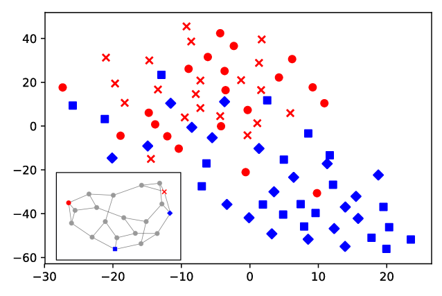
As explained in the intuitive explanation, rGINs can classify nodes correctly even if the random features are changed. We confirm this fact via visualization. We sample a test graph $G$ from TRIANGLE(N) and calculate the embedding of two positive nodes and two negative nodes using the trained rGINs in the TRIANGLE(N) experiment with $20$ different random seeds. Figure 2 visualizes the test graph $G$ and the scatter plot of the two-dimensional t-SNE embedding [27]. Red (circle and cross) nodes are positive examples, which have a triangle, and blue (square and diamond) nodes are negative examples. This figure shows that rGINs can correctly embed nodes even if the random features change. Note that Figure 2 is not completely linear separable because this projects the original $64$-dimensional embeddings into the $2$-dimensional space, and the learned parameters of rGINs are suboptimal.

In this paper, we show that the addition of the random features theoretically strengthens the capability of GINs. Especially, GINs with random features (rGINs) can distinguish any local substructures w.h.p. and solve the minimum dominating set problem and maximum matching problem with nearly optimal approximation ratios. The main advantage of rGINs is that they can guarantee the capability even with arbitrarily large test graphs. In the experiments, we show that rGINs can solve three problems that the normal GINs cannot solve, i.e., determining the existence of a triangle, computing local cluster coefficients, and learning an algorithm for the minimum dominating set problem. We also show that rGINs slightly outperform the normal GINs in biological real world datasets.

This work was supported by the JSPS KAKENHI GrantNumber 20H04243 and 20H04244.

We clarify the assumptions of theoretical results in detail. First, the number of dimensions is fixed but might be large, and we assume that the multi-layer perceptron is universal. These assumptions are stated in “there exist parameters ${\bm{\theta}}$” in the statements of theorems. The universal approximation theorem [8, 19, 18] justifies the latter assumption. Secondly, $p$ depends on the size of $R(G,v,L)$, but does not depend on the size of input graphs. Note that the size of $R(G,v,L)$ is bounded if $L$ and the maximum degree $\Delta$ are bounded.

Let $L\in\mathbb{Z}^{+}$ be an arbitrary positive integer and $\varepsilon>0$ be an arbitrary positive number. Let $p=\Delta^{-2(L+2)}\varepsilon$. $\forall\mu\in\mathcal{U}(p),\forall G=(V,E)\in\mathcal{F}(\Delta)\forall s,t\in V$, $Pr[{\bm{r}}_{s}={\bm{r}}_{t}]\leq p$. Because $|\mathcal{N}_{L}(v)|<\Delta^{L+2}$,

We construct $f(T)\in\mathcal{F}(\Delta)$. Let the node set $V^{\prime}$ be all ${\bm{r}}_{p}$ of level-$0$ sets $[{\bm{x}}_{p},{\bm{r}}_{p}]$ that $T[0]$ (i.e., the left element of $T$) contains, and the feature vector ${\bm{x}}^{\prime}_{{\bm{r}}_{p}}$ be equal to one of ${\bm{x}}_{p}$ (e.g., the smallest one). If for all $s,t\in\mathcal{N}_{L}(v)$, ${\bm{r}}_{s}\neq{\bm{r}}_{t}$ holds, the choice of ${\bm{x}}^{\prime}_{{\bm{r}}_{p}}$ is unique, and the number of nodes is the same as $G$. Let the center node be $v^{\prime}=T[0][0]\dots[0][1]$ (i.e., the right element of the leftmost level-$0$ set). $v^{\prime}$ is equal to ${\bm{r}}_{v}$ by construction. For $p,q\in V^{\prime}$, $\{p,q\}$ is included in $E^{\prime}$ if and only if there exists a level-$1$ set $T^{\prime}$ such that the right element of the left element of $T^{\prime}$ is equal to $p$, and a level-$0$ set whose right element is equal to $q$ is included in the right element of $T^{\prime}$. There exists an edge between $\{s,t\}\in E$ if and only if there exists an edge between $\{{\bm{r}}_{s},{\bm{r}}_{t}\}\in E^{\prime}$ by construction. Therefore, $f(T)=((V^{\prime},E^{\prime},{\bm{X}}^{\prime}),v^{\prime})\simeq(R(G,v,L),v)$ holds.          

From Corollary C.1 and Lemma C.2, for all $L\in\mathbb{Z}^{+}$, there exist parameters ${\bm{\theta}}$ of GINs such that for all $G=(V,E,{\bm{X}}),G^{\prime}=(V^{\prime},E^{\prime},{\bm{X}}^{\prime})\in\mathcal{F}(\Delta,C)$, ${\bm{R}}\in D^{|V|}$, ${\bm{R}}^{\prime}\in D^{|V^{\prime}|}$, $v\in V$, $v^{\prime}\in V^{\prime}$ if (1) for all $s,t\in\mathcal{N}_{L+1}(v)$, ${\bm{r}}_{s}\neq{\bm{r}}_{t}$, (2) for all $s^{\prime},t^{\prime}\in\mathcal{N}_{L+1}(v^{\prime})$, ${\bm{r}}_{s^{\prime}}\neq{\bm{r}}_{t^{\prime}}$, and (3) $(R(G,v,L),v)\not\simeq(R(G^{\prime},v^{\prime},L),v^{\prime})$ hold, $\textup{GIN}_{\bm{\theta}}((V,E,[{\bm{X}},{\bm{R}}]))_{v}\neq\textup{GIN}_{\bm{\theta}}((V^{\prime},E^{\prime},[{\bm{X}}^{\prime},{\bm{R}}^{\prime}]))_{v^{\prime}}$ holds. The cardinality of $\{R((V,E,[{\bm{X}},{\bm{R}}]),v,L)\mid G=(V,E,{\bm{X}})\in\mathcal{F}(\Delta,C),v\in V,{\bm{R}}\in D^{|V|}\}$ is finite. Therefore, there exists a multi layer perceptron MLP such that if the first and second conditions are valid, $\textup{MLP}(\textup{GIN}_{\bm{\theta}}((V,E,[{\bm{X}},{\bm{R}}]))_{v})>0.5$ if $\exists(G^{\prime},v^{\prime})\in\mathcal{G}$ such that $(G^{\prime},v^{\prime})\simeq(R(G,v,L),v)$ holds and $\textup{MLP}(\textup{GIN}_{\bm{\theta}}((V,E,[{\bm{X}},{\bm{R}}]))_{v})<0.5$ otherwise. This MLP can be considered as the last layer of the GIN. From Lemma C.1, there exists $p$ such that for all $\mu\in\mathcal{U}(p)$, the probability of the first and second conditions being true is arbitraily small.          

4.1 Let $U=\{v\in V\mid\exists u\in\mathcal{N}_{2}(v)\text{ s.t. }{\bm{r}}_{v}={\bm{r}}_{u}\}$ and $U^{+}=\{v\in V\mid\exists u\in\mathcal{N}(v)\text{ s.t. }u\in U\}$. The solution $S$ our sequential algorithm outputs for $G$ is the same as the union of $U^{+}$ and the solution $T$ the sequential algorithm [33, 26, 20] outputs for the induced graph $G^{\prime}$ of $V\backslash U^{+}$ by construction. From Lemma C.1, there exists $p$ such that for all $\mu\in\mathcal{U}(p)$, $|U|\leq\frac{\varepsilon}{\Delta+1}n$ with high probability. It means that $|U|\leq\varepsilon\textup{OPT}_{m}(\Pi_{\text{MDS}},G^{\prime})$ because for any $G=(V,E)\in\mathcal{F}(\Delta)$, $\textup{OPT}_{m}(\Pi_{\text{MDS}},G)\geq\frac{n}{\Delta+1}$ holds. Therefore, with high probability,

Let $S_{L}=\{v\in V\mid\text{the computation of }\mathcal{O}_{\Delta+1}(v)\text{ stops within }R(G,v,L)\}$, $U_{L}=\{v\in V\mid\exists s,t\in\mathcal{N}_{L}(v)\text{ s.t. }{\bm{r}}_{s}={\bm{r}}_{t}\}$, $A=\{v\in V\mid\mathcal{O}_{\Delta+1}(v)=1\}$. For fixed ${\bm{R}}$, let $f$ be a function that outputs $1$ if $v\in F=S_{L}\cup U_{L}\cup A$, and $0$ otherwise. This value can be computed only from $(R(G,v,L),v)$. From the locality lemma [33], there exists $L\in\mathbb{Z}^{+}$ such that $|S_{L}|\leq\frac{\varepsilon}{3(\Delta+1)}n\leq\frac{\varepsilon}{3}~\textup{OPT}_{m}(\Pi_{\text{MDS}},G)$ holds w.h.p. From Lemma C.1, $|U_{L}|\leq\frac{\varepsilon}{3(\Delta+1)}n\leq\frac{\varepsilon}{3}~\textup{OPT}_{m}(\Pi_{\text{MDS}},G)$ holds w.h.p. if $p$ is sufficiently large. From Lemma 4.1, there exists $p$ such that for all $\mu\in\mathcal{U}(p)$, $|A|\leq(H(\Delta+1)+\frac{\varepsilon}{3})~\textup{OPT}_{m}(\Pi_{\text{MDS}},G)$ holds w.h.p. $F$ always forms a dominating set because $A\subseteq F$. From the above equations, $|F|\leq|S_{L}|+|U_{L}|+|A|\leq(H(\Delta+1)+\varepsilon)~\textup{OPT}_{m}(\Pi_{\text{MDS}},G)$ holds w.h.p.          

From Corollary C.1, Lemma C.2, and Lemma 4.2, there exist parameters ${\bm{\theta}}$ of GINs such that $\forall G=(V,E)\in\mathcal{F}(\Delta)$, $\forall{\bm{R}}\in D^{|V|}$,

where $f$ is the function in the proof of Lemma 4.2. Therefore, rGINs can simulate $f$, which is $(H(\Delta+1)+\varepsilon)$-approximation w.h.p.          

Let $F=\{e=\{u,v\}\in E\mid\exists s,t\in\mathcal{N}_{t}(u)\cup\mathcal{N}_{t}(v)\text{ s.t. }{\bm{r}}_{s}={\bm{r}}_{t}\}$. The solution $S$ our sequential algorithm outputs for $G$ is the same as the solution $T$ the sequential algorithm [33] outputs for $G^{\prime}=(V,E\backslash F)$. Let $\varepsilon^{\prime}=\frac{\varepsilon}{2}$. From [33], the sequential algorithm [33] is $(1+\varepsilon^{\prime})$-approximation by setting $t=\text{ceil}(\frac{1}{\varepsilon^{\prime}})$. From Lemma C.1, there exists $p\in\mathbb{R}^{+}$ such that for all $\mu\in\mathcal{U}(p)$, $|F|\leq\frac{\varepsilon}{8(1+\varepsilon)^{2}\Delta}n$ because $|E|\leq\frac{\Delta}{2}n$ by the degree-bounded assumption. When an edge is added to the solution, at most $2\Delta$ candidate edges are excluded. Therefore,

holds. Furthermore,

holds. Therefore,

References

- [1] D. Angluin, Local and global properties in networks of processors, in STOC, 1980, pp. 82–93.
- [2] P. Barceló, E. V. Kostylev, M. Monet, J. Pérez, J. L. Reutter, and J. P. Silva, The logical expressiveness of graph neural networks, in ICLR, 2020.
- [3] I. I. Baskin, V. A. Palyulin, and N. S. Zefirov, A neural device for searching direct correlations between structures and properties of chemical compounds, Journal of Chemical Information and Computer Sciences, 37 (1997), pp. 715–721.
- [4] M. Bayati, J. H. Kim, and A. Saberi, A sequential algorithm for generating random graphs, Algorithmica, 58 (2010), pp. 860–910.
- [5] L. Becchetti, P. Boldi, C. Castillo, and A. Gionis, Efficient semi-streaming algorithms for local triangle counting in massive graphs, in KDD, 2008, pp. 16–24.
- [6] J. Bruna, W. Zaremba, A. Szlam, and Y. LeCun, Spectral networks and locally connected networks on graphs, in ICLR, 2014.
- [7] M. Chlebík and J. Chlebíková, Approximation hardness of dominating set problems in bounded degree graphs, Inf. Comput., 206 (2008), pp. 1264–1275.
- [8] G. Cybenko, Approximation by superpositions of a sigmoidal function, MCSS, 2 (1989), pp. 303–314.
- [9] G. Dasoulas, L. D. Santos, K. Scaman, and A. Virmaux, Coloring graph neural networks for node disambiguation, arXiv, abs/1912.06058 (2019).
- [10] M. Defferrard, X. Bresson, and P. Vandergheynst, Convolutional neural networks on graphs with fast localized spectral filtering, in NeurIPS, 2016, pp. 3837–3845.
- [11] R. Duh and M. Fürer, Approximation of k-set cover by semi-local optimization, in STOC, 1997, pp. 256–264.
- [12] J. Edmonds, Paths, trees, and flowers, Canadian Journal of mathematics, 17 (1965), pp. 449–467.
- [13] J. Gilmer, S. S. Schoenholz, P. F. Riley, O. Vinyals, and G. E. Dahl, Neural message passing for quantum chemistry, in ICML, 2017, pp. 1263–1272.
- [14] Y. Gong, Y. Zhu, L. Duan, Q. Liu, Z. Guan, F. Sun, W. Ou, and K. Q. Zhu, Exact-k recommendation via maximal clique optimization, in KDD, 2019, pp. 617–626.
- [15] M. Gori, G. Monfardini, and F. Scarselli, A new model for learning in graph domains, in Proceedings of the International Joint Conference on Neural Networks, IJCNN, vol. 2, 2005, pp. 729–734.
- [16] A. Hagberg, P. Swart, and D. S Chult, Exploring network structure, dynamics, and function using networkx, in Proceedings of the 7th Python in Science Conference, SciPy, 2008, pp. 11–15.
- [17] L. Hella, M. Järvisalo, A. Kuusisto, J. Laurinharju, T. Lempiäinen, K. Luosto, J. Suomela, and J. Virtema, Weak models of distributed computing, with connections to modal logic, in PODC, 2012, pp. 185–194.
- [18] K. Hornik, Approximation capabilities of multilayer feedforward networks, Neural Networks, 4 (1991), pp. 251–257.
- [19] K. Hornik, M. B. Stinchcombe, and H. White, Multilayer feedforward networks are universal approximators, Neural Networks, 2 (1989), pp. 359–366.
- [20] D. S. Johnson, Approximation algorithms for combinatorial problems, J. Comput. Syst. Sci., 9 (1974), pp. 256–278.
- [21] N. Keriven and G. Peyré, Universal invariant and equivariant graph neural networks, in NeurIPS, 2019, pp. 7090–7099.
- [22] D. P. Kingma and J. Ba, Adam: A method for stochastic optimization, in ICLR, 2015.
- [23] T. N. Kipf and M. Welling, Semi-supervised classification with graph convolutional networks, in ICLR, 2017.
- [24] D. Liben-Nowell and J. M. Kleinberg, The link prediction problem for social networks, in CIKM, 2003, pp. 556–559.
- [25] A. Loukas, What graph neural networks cannot learn: depth vs width, in ICLR, 2020.
- [26] L. Lovász, On the ratio of optimal integral and fractional covers, Discrete Mathematics, 13 (1975), pp. 383–390.
- [27] L. v. d. Maaten and G. Hinton, Visualizing data using t-sne, J. Mach. Learn. Res., 9 (2008), pp. 2579–2605.
- [28] H. Maron, H. Ben-Hamu, H. Serviansky, and Y. Lipman, Provably powerful graph networks, in NeurIPS, 2019, pp. 2153–2164.
- [29] H. Maron, E. Fetaya, N. Segol, and Y. Lipman, On the universality of invariant networks, in ICML, 2019, pp. 4363–4371.
- [30] C. Morris, M. Ritzert, M. Fey, W. L. Hamilton, J. E. Lenssen, G. Rattan, and M. Grohe, Weisfeiler and leman go neural: Higher-order graph neural networks, in AAAI, 2019, pp. 4602–4609.
- [31] R. L. Murphy, B. Srinivasan, V. A. Rao, and B. Ribeiro, Janossy pooling: Learning deep permutation-invariant functions for variable-size inputs, in ICLR, 2019.
- [32] , Relational pooling for graph representations, in ICML, 2019, pp. 4663–4673.
- [33] H. N. Nguyen and K. Onak, Constant-time approximation algorithms via local improvements, in FOCS, 2008, pp. 327–336.
- [34] M. Niepert, M. Ahmed, and K. Kutzkov, Learning convolutional neural networks for graphs, in ICML, 2016, pp. 2014–2023.
- [35] M. Parnas and D. Ron, Approximating the minimum vertex cover in sublinear time and a connection to distributed algorithms, Theor. Comput. Sci., 381 (2007), pp. 183–196.
- [36] R. Rubinfeld and A. Shapira, Sublinear time algorithms, SIAM J. Discrete Math., 25 (2011), pp. 1562–1588.
- [37] R. Sato, A survey on the expressive power of graph neural networks, arXiv, (2020).
- [38] R. Sato, M. Yamada, and H. Kashima, Approximation ratios of graph neural networks for combinatorial problems, in NeurIPS, 2019, pp. 4083–4092.
- [39] F. Scarselli, M. Gori, A. C. Tsoi, M. Hagenbuchner, and G. Monfardini, The graph neural network model, IEEE Trans. Neural Networks, 20 (2009), pp. 61–80.
- [40] M. S. Schlichtkrull, T. N. Kipf, P. Bloem, R. van den Berg, I. Titov, and M. Welling, Modeling relational data with graph convolutional networks, in The Semantic Web - 15th International Conference, ESWC, 2018, pp. 593–607.
- [41] D. I. Shuman, S. K. Narang, P. Frossard, A. Ortega, and P. Vandergheynst, The emerging field of signal processing on graphs: Extending high-dimensional data analysis to networks and other irregular domains, IEEE Signal Process. Mag., 30 (2013), pp. 83–98.
- [42] A. Sperduti and A. Starita, Supervised neural networks for the classification of structures, IEEE Trans. Neural Networks, 8 (1997), pp. 714–735.
- [43] J. Suomela, Survey of local algorithms, ACM Comput. Surv., 45 (2013), pp. 24:1–24:40.
- [44] H. Wang, M. Zhao, X. Xie, W. Li, and M. Guo, Knowledge graph convolutional networks for recommender systems, in WWW, 2019, pp. 3307–3313.
- [45] X. Wang, X. He, Y. Cao, M. Liu, and T. Chua, KGAT: knowledge graph attention network for recommendation, in KDD, 2019, pp. 950–958.
- [46] D. J. Watts and S. H. Strogatz, Collective dynamics of ‘small-world’networks, nature, 393 (1998), p. 440.
- [47] B. Weisfeiler and A. A. Lehman, A reduction of a graph to a canonical form and an algebra arising during this reduction, Nauchno-Technicheskaya Informatsia, 2 (1968), pp. 12–16.
- [48] H. T. Welser, E. Gleave, D. Fisher, and M. A. Smith, Visualizing the signatures of social roles in online discussion groups, Journal of Social Structure, 8 (2007).
- [49] K. Xu, W. Hu, J. Leskovec, and S. Jegelka, How powerful are graph neural networks?, in ICLR, 2019.
- [50] R. Ying, R. He, K. Chen, P. Eksombatchai, W. L. Hamilton, and J. Leskovec, Graph convolutional neural networks for web-scale recommender systems, in KDD, 2018, pp. 974–983.
A Experimental Setups
A.1 Dataset Descriptions
- •
MUATG is a chemical compound dataset. Each node represents an atom and each edge represents a chemical bond. A node feature vector is a one-hot vector that represents an atom type. Graphs are labelled according to their mutagenic effect on a bacterium.
NCI1 is a chemical compound dataset. Each node represents an atom and each edge represents a chemical bond. A node feature vector is a one-hot vector that represents an atom type. Graphs are labelled according to the bioassay records for anti-cancer screen tests with non-small cell lung.
PROTEINS is a protein dataset. Each nodes represents a secondary structure element, and a node feature vector is a one-hot vector that represents a structure type (helix, sheet, or turn). Two nodes are connected if they are neighbors either in the amid acid sequence or in 3D space. Graphs are labelled according to whether they are enzymes or non-enzymes.
A.2 General Setups
In the experiments, we use five-layered GNNs (including the input layer). In our experiments, the graph convolutional networks (GCNs) aggregate the features by average pooling, following [49] whereas the original model [23] uses symmetrized normalization. We train models with the Adam optimizer [22] with an initial learning rate of and batch size of . We decay the learning rate by every epochs. We use dropout in the final layer with a dropout rate of for graph classification datasets (i.e., MUTAG, NCI1, and PROTEINS). We do not train the parameters because the authors of [49] showed that it does not affect the performance. We train models for epochs for the TRIANGLE and LCC datasets, and select the number of epochs from by cross-validation for MUTAG, NCI1, and PROTEINS datasets. It is noteworthy that these hyperparamter settings are the default values of the open implementation of GINs https://github.com/weihua916/powerful-gnns, which have been shown to be effective in practice.
Setups for MDS. We use different hyperparameters in the MDS experiments because learning the greedy algorithm requires more expressive power. Specifically, we use ten-layered GNNs with hidden dimensions. We train the model with SGD with learning rate for epochs.
A.3 Graph Synthesis Process
We generate graphs for TRIANGLE, LCC, and MDS datasets by the random_degree_sequence_graph function of networkx package [4, 16]. All graphs are generated by the same process with different seeds. Figure 3 shows examples of test graphs of the TRIANGLE(S) dataset.
B More Discussion on Assumptions