Higher-order exceptional points in all-magnetic structures

The magnetometer, for measuring the intensity of magnetic fields, was firstly created by Carl Friedrich Gauss in 1833 Gauss1832 and received tremendous progress since then. It has been widely utilized in mineral explorations Sharma1987; Hato2013, accelerator physics Arpaia2018, archaeology Fassbinder2016, mobile phones Cai2012, etc. A long-term goal in the community is to pursue magnetometers with ultrahigh sensitivity. Conventional techniques in magnetic sensors encompass many aspect of physics. For example, fluxgate magnetometer works due to the nonlinear character of soft magnetic materials when they are saturated Primdahl1979; Acuna1974. Magnetoresistive devices typically are made of thin strips of permalloy whose electrical resistance varies with external magnetic fields Caruso1997. Although different magnetometric devices are designed based on different physical mechanisms, they share a general rule that the variation of the order parameter linearly varies with respect to the magnetic field. Presently, ultrahigh-sensitive magnetometers like superconducting quantum interference devices can reach a magnetic sensitivity of $1\text{fT}/\text{Hz}^{1/2}$, but they require an extreme low working temperature and an oversized volume Gallop2003; Kleiner2004. Seeking a solid state, small size, room temperature magnetometer with ultrahigh sensitivity is thus one central issue. Recently, it has been demonstrated that the peculiar non-Hermitian degeneracy in magnetic structures Lee2015; Yang2018; Cao2019; Liu2019; Yuan2020 may provide a promising way to solve the problem.

Hamiltonian obeying the parity-time ($\mathcal{PT}$) symmetry constitutes a special non-Hermitian system, which is invariant under combined parity $\mathcal{P}$ and time-reversal $\mathcal{T}$ operations. It has attracted a lot of attention due to both the fundamental interest in quantum theory Bender1998; Bender2007; Konotop2016 and the promising application in many fields Hodaei2017; Feng2014; Hodaei2014, such as optics Makris2008; Guo2009; Ruter2010, tight-binding modeling Bendix2009; Joglekar2010, acoustics Zhu2014; Jing2014, electronics Schindler2011; Choi2018, and very recently in spintronics Lee2015; Yang2018; Cao2019; Liu2019; Yuan2020. A $\mathcal{PT}$-symmetric Hamiltonian could exhibit entirely real spectra and a spontaneous symmetry breaking accompanied by a real-to-complex spectra phase transition at the exceptional point (EP) where two or more eigenvalues and their corresponding eigenvectors coalesce simultaneously. In the vicinity of the EP, the eigenfrequency shift follows the $1/N$ power law of the external perturbation, where $N$ is the order of the EP. Such a feature can significantly enhance the sensitivity and has been observed by several experiments Chen2017; Hodaei2017; Chen2018; Chen20182; Zeng2019.

$\mathcal{PT}$ symmetry and EP in magnetic systems are receiving growing recent interests. In a simple bilayer structure of two macrospins with balanced gain and loss, the second-order EP (EP2) was observed at a critical Gilbert damping constant Lee2015. In Ref. Zhang2018, it was proposed to realize the pseudo-Hermiticity in a cavity magnonics system with the third-order EP (EP3). By taking the spin-wave excitation into account, some of the present authors reported a novel ferromagnetic to antiferromagnetic (AFM) phase transition at the EP that depends on magnon’s wave vector Yang2018. In Ref. Cao2019, an exceptional magnetic sensitivity was predicted in the vicinity of the EP3 for $\mathcal{PT}$-symmetric cavity magnon polaritons. However, high-order EPs in purely magnetic/magnonic system is yet to be explored.

In this work, we propose a ferromagnetic trilayer structure consisting of a gain, a neutral, and a loss layer to achieve the EP3. We show that, in the vicinity of the EP3, the separation of eigenfrequencies follow a power law $\Delta\omega_{\text{EP3}}\propto\epsilon^{1/3}$. Here, the perturbation $\epsilon$ comes from the disturbing magnetic field. We find mode-dependent EPs when the spin-wave excitation is allowed by including the intralayer exchange coupling. A ferromagnetic-to-antiferromagnetic phase transition is observed when the $\mathcal{PT}$ symmetry is broken. Our results suggest a promising way to realize higher-order non-Hermitian degeneracy in a purely magnetic system and to design magnetometer with ultrahigh sensitivities.

The paper is organized as follows: Section II gives the macrospin model. The condition for observing EP3 is analytically derived. The one-half and one-third power law around EP2 and EP3 are demonstrated, respectively. The effect of noise on the magnetic sensitivity is analyzed as well. In Sec. III, we extend the idea to ferromagnetic trilayers, by allowing spin-wave excitations. Discussion and conclusion are drawn in Sec. IV.

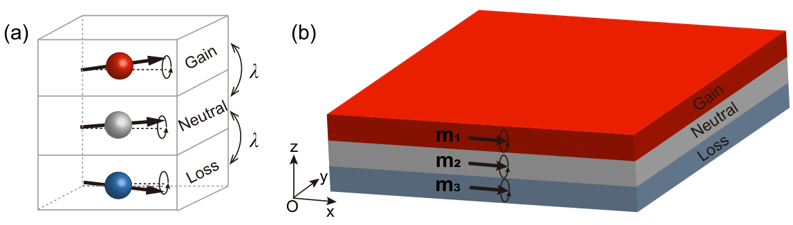
We first consider a ternary macrospin structure shown in Fig. 1(a). The Hamiltonian contains the Zeeman energy, magnetic anisotropy, and exchange coupling:

$$\mathcal{H}=-\sum_{n}{\bf B}\cdot{\bf M}_{n}-\sum_{n}\frac{K_{n}}{2}(m^{x}_{n})^{2}-\lambda\mu_{0}{\bf M}_{2}\cdot({\bf M}_{1}+{\bf M}_{3}),$$

(1)

where ${\bf M}_{n}$ (${\bf m}_{n}={\bf M}_{n}/M_{n}$) is the spin (unit spin) with subscript index $n$ labeling the $n$-th layer ($n=1,2,3$), $M_{n}$ is the saturated magnetization, ${\bf B}=B\hat{x}$ is the external magnetic field applied on the whole structure, $K_{n}>0$ is the uniaxial anisotropy, ${\lambda>0}$ is the ferromagnetic exchange-coupling strength between two adjacent layers, and $\mu_{0}$ is the vacuum permeability. The top and bottom layers are assumed to be the same material but with opposite Gilbert damping parameters, to guarantee the $\mathcal{PT}$ symmetry. The coupled magnetization dynamics is described by the Landau-Lifshitz-Gilbert (LLG) equation Wang20091; Wang20092:

	$\displaystyle\frac{\partial{\bf m}_{1}}{\partial t}$	$\displaystyle=$	$\displaystyle-\gamma{\bf m}_{1}\times{\bf B}_{\text{eff,1}}-\alpha{\bf m}_{1}\times\frac{\partial{\bf m}_{1}}{\partial t},$		(2a)
	$\displaystyle\frac{\partial{\bf m}_{2}}{\partial t}$	$\displaystyle=$	$\displaystyle-\gamma{\bf m}_{2}\times{\bf B}_{\text{eff,2}},$		(2b)
	$\displaystyle\frac{\partial{\bf m}_{3}}{\partial t}$	$\displaystyle=$	$\displaystyle-\gamma{\bf m}_{3}\times{\bf B}_{\text{eff,3}}+\alpha{\bf m}_{3}\times\frac{\partial{\bf m}_{3}}{\partial t},$		(2c)

where $\gamma$ is the gyromagnetic ratio, $\alpha>0$ is the Gilbert constant employed as the balanced gain-loss parameter. The effective magnetic fields read:

	$\displaystyle{\bf B}_{\text{eff,1}}$	$\displaystyle=$	$\displaystyle{B}\hat{x}+\frac{K_{1}}{M_{1}}{m}_{1}^{x}\hat{x}+\lambda\mu_{0}M_{2}{\bf m}_{2},$		(3a)
	$\displaystyle{\bf B}_{\text{eff,2}}$	$\displaystyle=$	$\displaystyle{B}\hat{x}+\frac{K_{2}}{M_{2}}{m}_{2}^{x}\hat{x}+\lambda\mu_{0}M_{1}({\bf m}_{1}+{\bf m}_{3}),$		(3b)
	$\displaystyle{\bf B}_{\text{eff,3}}$	$\displaystyle=$	$\displaystyle{B}\hat{x}+\frac{K_{1}}{M_{1}}{m}_{3}^{x}\hat{x}+\lambda\mu_{0}M_{2}{\bf m}_{2}.$		(3c)

For small-amplitude spatiotemporal magnetization precession, we assume ${\bf m}_{n}=\hat{x}+m^{y}_{n}\hat{y}+m^{z}_{n}\hat{z}$ with $|m^{y,z}_{n}|\ll 1$. By substituting Eqs. (3) into Eqs. (2), and introducing $\psi_{n}=m^{y}_{n}-im^{z}_{n}$, we obtain

	$\displaystyle(i+\alpha)\dot{\psi}_{1}$	$\displaystyle=$	$\displaystyle\omega_{1}\psi_{1}-\omega_{\lambda 2}\psi_{2},$		(4a)
	$\displaystyle i\dot{\psi}_{2}$	$\displaystyle=$	$\displaystyle-\omega_{\lambda 1}\psi_{1}+\omega_{2}\psi_{2}-\omega_{\lambda 1}\psi_{3},$		(4b)
	$\displaystyle(i-\alpha)\dot{\psi}_{3}$	$\displaystyle=$	$\displaystyle-\omega_{\lambda 2}\psi_{2}+\omega_{1}\psi_{3},$		(4c)

where $\omega_{1}=\gamma(B+K_{1}/M_{1}+\lambda\mu_{0}M_{2})$, $\omega_{2}=\gamma(B+K_{2}/M_{2}+2\lambda\mu_{0}M_{1})$, $\omega_{\lambda 1}=\gamma\lambda\mu_{0}M_{1}$, and $\omega_{\lambda 2}=\gamma\lambda\mu_{0}M_{2}$. Imposing a harmonic time-dependence $\psi_{n}=\phi_{n}\exp(-i\omega t)$, we have the secular equation:

$$\omega\phi=H\phi,$$

(5)

with $\phi=(\phi_{1},\phi_{2},\phi_{3})^{\text{T}}$, and

$$H=\left(\begin{array}[]{ccc}\frac{\omega_{1}}{1-i\alpha}&-\frac{\omega_{\lambda 2}}{1-i\alpha}&0\\ -\omega_{\lambda 1}&\omega_{2}&-\omega_{\lambda 1}\\ 0&-\frac{\omega_{\lambda 2}}{1+i\alpha}&\frac{\omega_{1}}{1+i\alpha}\\ \end{array}\right).$$

(6)

In this section, we extend the macrospin model to trilayer ferromagnets which include both intralayer and interlayer exchange couplings, as shown in Fig. 1(b). The Hamiltonian of the system is then given by:

	$\displaystyle\mathcal{H}=$	$\displaystyle-\sum_{n}\sum_{<i,j>}J_{n}{\bf m}_{n,i}\cdot{\bf m}_{n,j}-\sum_{n}\sum_{i}{\bf B}_{n,i}\cdot{\bf M}_{n,i}$		(19)
		$\displaystyle-\sum_{n}\sum_{i}\frac{K_{n}}{2}(m^{x}_{n,i})^{2}-\lambda\mu_{0}\sum_{i}{\bf M}_{2,i}\cdot({\bf M}_{1,i}+{\bf M}_{3,i}),$

where ${\bf M}_{n,i}$ (${\bf{m}}_{n,i}={\bf M}_{n,i}/M_{n,i}$) is the spin (unit spin) at the $i$-th site in the $n$-th layer ($n=1,2,3$) with the saturation magnetization $M_{n,i}$, $J_{n}>0$ is the intralayer exchange coupling constant, $\langle i,j\rangle$ sums over all nearest-neighbor sites in the same layer, and ${\bf B}_{n,i}=B_{n,i}\hat{x}$ is the external magnetic field at the $i$-th site in the $n$-th layer. In the calculations, we adopt the same material parameters as the macrospin model and consider the intralayer exchange coupling constant $J_{1,2,3}=J=2.44\times 10^{7}$ J/m³. A homogeneous magnetic field is assumed to be applied over the whole system, i.e., $B_{1,i}=B_{2,i}=B_{3,i}=B$.

The magnetization dynamics is described by the LLG equation (2) but with the following effective fields:

	$\displaystyle{\bf B}_{\text{eff,1,i}}$	$\displaystyle=\frac{J}{M_{1}}\sum_{<i,j>}{\bf m}_{1,j}+B\hat{x}+\frac{K_{1}}{M_{1}}{m}_{1}^{x}\hat{x}+\lambda\mu_{0}M_{2}{\bf m}_{2,i},$		(20)
	$\displaystyle{\bf B}_{\text{eff,2,i}}$	$\displaystyle=\frac{J}{M_{2}}\sum_{<i,j>}{\bf m}_{2,j}+B\hat{x}+\frac{K_{2}}{M_{2}}{m}_{2}^{x}\hat{x}+\lambda\mu_{0}M_{1}({\bf m}_{1,i}+{\bf m}_{3,i}),$
	$\displaystyle{\bf B}_{\text{eff,3,i}}$	$\displaystyle=\frac{J}{M_{1}}\sum_{<i,j>}{\bf m}_{3,j}+B\hat{x}+\frac{K_{1}}{M_{1}}{m}_{3}^{x}\hat{x}+\lambda\mu_{0}M_{2}{\bf m}_{2,i},$

where $J\sum_{<i,j>}{\bf m}_{n,j}$ represents $J[{\bf m}_{n,(i_{x}-1)a,i_{y}a}+{\bf m}_{n,(i_{x}+1)a,i_{y}a}+{\bf m}_{n,i_{x}a,(i_{y}-1)a}+{\bf m}_{n,i_{x}a,(i_{y}+1)a}]$ with $(i_{x}a,i_{y}a)$ being the coordinate of the $i$-th unit spin vector, $i_{x(y)}$ is an integer, and $a$ is the lattice constant.

Considering a small-angle dynamics, we set ${\bf m}_{n,i}=\hat{x}+m^{y}_{n,i}\hat{y}+m^{z}_{n,i}\hat{z}$ with $|m^{y,z}_{n,i}|\ll 1$. Substituting the effective field into Eqs. (2) and imposing the complex scalar-fields $\psi_{n,i}=m^{y}_{n,i}-im^{z}_{n,i}$, we obtain:

	$\displaystyle i\dot{\psi}_{1,i}$	$\displaystyle=\frac{\gamma J}{M_{1}}\left(4\psi_{1,i}-\sum_{<i,j>}\psi_{1,j}\right)+\omega_{\lambda 2}\left(\psi_{1,i}-\psi_{2,i}\right)+\gamma\left(B+\frac{K_{1}}{M_{1}}\right)\psi_{1,i}-\alpha\dot{\psi}_{1,i},$		(21)
	$\displaystyle i\dot{\psi}_{2,i}$	$\displaystyle=\frac{\gamma J}{M_{2}}\left(4\psi_{2,i}-\sum_{<i,j>}\psi_{2,j}\right)+\omega_{\lambda 1}\left(2\psi_{2,i}-\psi_{1,i}-\psi_{3,i}\right)+\gamma\left(B+\frac{K_{2}}{M_{2}}\right)\psi_{2,i},$
	$\displaystyle i\dot{\psi}_{3,i}$	$\displaystyle=\frac{\gamma J}{M_{1}}\left(4\psi_{3,i}-\sum_{<i,j>}\psi_{3,j}\right)+\omega_{\lambda 2}\left(\psi_{3,i}-\psi_{2,i}\right)+\gamma\left(B+\frac{K_{1}}{M_{1}}\right)\psi_{3,i}+\alpha\dot{\psi}_{3,i},$

with the abbreviation $\sum_{<i,j>}{\psi}_{n,j}={\psi}_{n,(i_{x}-1)a,i_{y}a}+{\psi}_{n,(i_{x}+1)a,i_{y}a}+{\psi}_{n,i_{x}a,(i_{y}-1)a}+{\psi}_{n,i_{x}a,(i_{y}+1)a}$.

Expanding the spatiotemporal magnetization in terms of plan waves $\psi_{n,i}=\phi_{n,i}\exp(i{\bf k}\cdot{\bf r}-i\omega t)$, we have:

$$\omega\phi_{i}=H_{i}\phi_{i},$$

(22)

with

$$H_{i}=\left(\begin{array}[]{ccc}\frac{\omega^{\prime}_{1}}{1-i\alpha}&-\frac{\omega_{\lambda 2}}{1-i\alpha}&0\\ -\omega_{\lambda 1}&\omega^{\prime}_{2}&-\omega_{\lambda 1}\\ 0&-\frac{\omega_{\lambda 2}}{1+i\alpha}&\frac{\omega^{\prime}_{1}}{1+i\alpha}\\ \end{array}\right),$$

(23)

and $\phi_{i}=(\phi_{1,i},\phi_{2,i},\phi_{3,i})^{\text{T}}$, where $\omega^{\prime}_{1}=\tilde{\omega}_{1}(k_{x},k_{y})+\gamma(B+K_{1}/M_{1}+\lambda\mu_{0}M_{2})$ and $\omega^{\prime}_{2}=\tilde{\omega}_{2}(k_{x},k_{y})+\gamma(B+K_{2}/M_{2}+2\lambda\mu_{0}M_{1})$ with $\tilde{\omega}_{n}(k_{x},k_{y})=2\gamma J/M_{n}\left[2-\cos(k_{x}a)-\cos(k_{y}a)\right]$.

It is straightforward to see that, for $k_{x}=k_{y}=0$, Eq. (22) is reduced to Eq. (5). We aim to search for all EPs in ferromagnetic trilayers. Following Ref. Yang2018, we know that the emergence of EP3 depends on magnon’s wave vector $\mathbf{k}=(k_{x},k_{y})$. As two examples, we set $\mathbf{k}=(\frac{\pi}{30a},0)$ and $(\frac{\pi}{20a},0)$ without loss of generality, to illustrate the condition supporting the EP3, which are depicted in Fig. 6 (a) and Fig. 6(b), respectively. We then explicitly demonstrate the emergence of EP3 in Fig. 6(c) and Fig. 6(d). We observe that the EP2 appears for all spin-wave modes. At a given $(k_{x},k_{y})$, there exists a critical gain-loss parameter $\alpha_{c}$, beyond which the exact $\mathcal{PT}$ symmetry is broken. We plot the distribution of the critical gain-loss parameter over the entire Brillouin zone in Fig. 7(a). The red circle marks the critical $\alpha$ for the emergence of EP3. In comparison to previous work Yang2018, we did not note a special region where the $\mathcal{PT}$ symmetry is never broken. This is due to the fact that the chiral spin-spin coupling, i.e., Dzyaloshinskii-Moriya interaction, is absent in the present model.

As first predicted in Ref. Yang2018, for a $\mathcal{PT}$-symmetry ferromagnetic bilayer, antiferromagnetism could emerge in the $\mathcal{PT}$ broken phase. As to the ferromagnetic trilayer, it can exhibit a FM-AFM phase transition as well. In Fig. 7(a), we find that the minimum of $\alpha_{c}$(k) appears at the boundary of the Brillouin zone. We calculate the corresponding critical gain-loss parameter at ${\bf k}=(\pm\frac{\pi}{a},\pm\frac{\pi}{a})$ for different $\lambda$,

$$\alpha_{c}=\sqrt{X(\textbf{k})-1}\left|{}_{{\bf k}=(\pm\frac{\pi}{a},\pm\frac{\pi}{a})},\right.$$

(24)

where

$$X=\frac{1}{12\omega^{\prime 3}_{2}\left(\omega^{\prime 2}_{1}\omega^{\prime}_{2}-2\omega^{\prime}_{1}\omega_{\lambda 1}\omega_{\lambda 2}\right)}\left[c_{1}+\left(c_{3}-\sqrt{c_{3}^{2}-c_{2}^{3}}\right)^{1/3}+\left(c_{3}+\sqrt{c_{3}^{2}-c_{2}^{3}}\right)^{1/3}\right],\\$$

(25)

with

$$\begin{split}&c_{1}=-27\beta_{1}^{2}-6\beta_{1}\omega^{\prime}_{2}\left(3\beta_{2}+4\omega^{\prime}_{1}\omega^{\prime}_{2}\right)+\beta_{2}^{2}\omega^{\prime 2}_{2},\\ &c2=\left[27\beta_{1}^{2}+6\beta_{1}\omega^{\prime}_{2}\left(3\beta_{2}+4\omega^{\prime}_{1}\omega^{\prime}_{2}\right)-\beta_{2}^{2}\omega^{\prime 2}_{2}\right]^{2}-48\beta_{1}\omega^{\prime 3}_{2}(9\beta_{1}\beta_{2}\omega^{\prime}_{1}+12\beta_{1}\omega^{\prime 2}_{1}\omega^{\prime}_{2}-\beta_{2}^{3}-\beta_{2}^{2}\omega^{\prime}_{1}\omega^{\prime}_{2}),\\ &c3=-\left[27\beta_{1}^{2}+6\beta_{1}\omega^{\prime}_{2}\left(3\beta_{2}+4\omega^{\prime}_{1}\omega^{\prime}_{2}\right)-\beta_{2}^{2}\omega^{\prime 2}_{2}\right]^{3}+72\beta_{1}\omega^{\prime 3}_{2}\left[27\beta_{1}^{2}+6\beta_{1}\omega^{\prime}_{2}\left(3\beta_{2}+4\omega^{\prime}_{1}\omega^{\prime}_{2}\right)-\beta_{2}^{2}\omega^{\prime 2}_{2}\right]\\ &\ \ \ \ \ \ \ \ \times\left(9\beta_{1}\beta_{2}\omega^{\prime}_{1}+12\beta_{1}\omega^{\prime 2}_{1}\omega^{\prime}_{2}-\beta_{2}^{3}-\beta_{2}^{2}\omega^{\prime}_{1}\omega^{\prime}_{2}\right)-864\beta_{1}^{2}\omega^{\prime 2}_{1}\omega^{\prime 6}_{2}\left(8\beta_{1}\omega^{\prime}_{1}-\beta_{2}^{2}\right),\\ &\beta_{1}=\omega^{\prime 2}_{1}\omega^{\prime}_{2}-2\omega^{\prime}_{1}\omega_{\lambda 1}\omega_{\lambda 2},\\ &\beta_{2}=2\omega_{\lambda 1}\omega_{\lambda 2}-\omega^{\prime 2}_{1}-2\omega^{\prime}_{1}\omega^{\prime}_{2},\end{split}$$

(26)

as plotted by the solid black curve in Fig. 7(b), in which the blue and red regions represent the AFM and FM phases, respectively. The phase boundary for $\mathcal{PT}$-symmetric bilayer is

$$\alpha_{c}=\frac{\lambda\mu_{0}M_{1}}{\sqrt{\frac{8J}{M_{1}}+B+\frac{K_{1}}{M_{1}}}\sqrt{\frac{8J}{M_{1}}+B+\frac{K_{1}}{M_{1}}+2\lambda\mu_{0}M_{1}}}$$

(27)

marked by the dashed line in Fig. 7(b), as a comparison.

Negative damping (gain) is the key to realize our proposal. In previous work Lee2015; Yang2018, it has been suggested that the spin transfer torque, the parametric driving, the ferromagnetic$|$ferroelectric heterostructure Jia2015, and the interaction between magnetic system and environment Ando2008; Duan2014; Li2014 are possible mechanisms to achieve the magnetic gain. Slavin et al. analytically demonstrated that the main effect of the spin-polarized current in a “free” magnetic layer is a negative damping Slavin2005. In Ref. Apalkov2005, the Slonczewski form of the spin torque is treated as a negative damping too.

To achieve the EP3, FM coupling between two adjacent layers should fall into the allowed parametric space, which can be realized by tuning the thickness of the nonmagnetic spacer between them Frackowiak2018; Vincent2002. A single-mode spin wave can be excited via the Brillouin light scattering technique Park2002; Dem2001, which is essential to observe the mode-dependent EP3.

In summary, we have theoretically investigated the dynamics of $\mathcal{PT}$-symmetric ternary macrospin structure and ferromagnetic trilayer. We observed both EP2 and EP3 under proper materials parameters. We demonstrated the one-half and one-third power law response to external perturbations in the vicinity of EP2 and EP3, respectively. Outstanding magnetic sensitivities were identified in the vicinity of EP3. Our results open the door for observing higher-order EPs in all-magnetic structures and for designing ultrahigh-sensitive magnetometers.

This work was supported by the National Natural Science Foundation of China (Grants No. 11704060 and No. 11604041).

References

- (1) C. F. Gauss, The Intensity of the Earth’s Magnetic Force Reduced to Absolute Measurement, Royal Scientific Society 8, 3 (1832).
- (2) P. V. Sharma, Magnetic method applied to mineral exploration, Ore Geol. Rev. 2, 323 (1987).
- (3) T. Hato, A. Tsukamoto, S. Adachi, Y. Oshikubo, H. Watanabe, H. Ishikawa, M. Sugisaki, E. Arai, and K. Tanabe, Development of HTS-SQUID magnetometer system with high slew rate for exploration of mineral resources, Supercond. Sci. Technol. 26, 115003 (2013).
- (4) P. Arpaia, G. Caiafa, and S. Russenschuck, A rotating-coil magnetometer for the scanning of transversal field harmonics in particle accelerator magnets, J. Phys.: Conf. Ser. 1065, 052046 (2018).
- (5) A. S. Gilbert, Magnetometry for Archaeology, Encyclopaedia of Geoarchaeolog (Springer, Netherlands, 2016).
- (6) Y. Cai, Y. Zhao, X. Ding, and J. Fennelly, Magnetometer basics for mobile phone applications, Electron. Prod. (Garden City, New York) 54, 2 (2012).
- (7) F. Primdahl, The fluxgate magnetometer, J. Phys. E: Sci. Instrum 12, 241 (1979).
- (8) M. Acuna, Fluxgate magnetometers for outer planets exploration, IEEE Trans. Magn. 10, 519 (1974).
- (9) M. J. Caruso, Applications of Magnetoresistive Sensors in Navigation Systems, SAE Technical Paper (1997).
- (10) J. Gallop, SQUIDs: Some limits to measurement, Supercond. Sci. Technol. 16 1575 (2003).
- (11) R. Kleiner, D. Koelle, F. Ludwig, and J. Clarke, Superconducting quantum interference devices: State of the art and applications, Proc. IEEE 92 1534 (2004).
- (12) J. M. Lee, T. Kottos, and B. Shapiro, Macroscopic magnetic structures with balanced gain and loss, Phys. Rev. B 91, 094416 (2015).
- (13) H. Yang, C. Wang, T. Yu, Y. Cao, and P. Yan, Antiferromagnetism Emerging in a Ferromagnet with Gain, Phys. Rev. Lett. 121, 197201 (2018).
- (14) Y. Cao and P. Yan, Exceptional magnetic sensitivity of -symmetric cavity magnon polaritons, Phys. Rev. B 99, 214415 (2019).
- (15) H. Liu, D. Sun, C. Zhang, M. Groesbeck, R. Mclaughlin, and Z. V. Vardeny, Observation of exceptional points in magnonic parity-time symmetry devices, Sci. Adv. 5, eaax9144 (2019).
- (16) H. Y. Yuan, P. Yan, S. Zheng, Q. Y. He, K. Xia, and M.-H. Yung, Steady Bell State Generation via Magnon-Photon Coupling, Phys. Rev. Lett. 124, 053602 (2020).
- (17) C. M. Bender and S. Boettcher, Real Spectra in Non-Hermitian Hamiltonians Having Symmetry, Phys. Rev. Lett. 80, 5243 (1998).
- (18) C. M. Bender, D. C. Brody, H. F. Jones, and B. K. Meister, Faster than Hermitian Quantum Mechanics, Phys. Rev. Lett. 98, 040403 (2007).
- (19) V. V. Konotop, J. Yang, and D. A. Zezyulin, Nonlinear waves in -symmetric systems, Rev. Mod. Phys. 88, 035002 (2016).
- (20) H. Hodaei, A. U. Hassan, S. Wittek, H. Garcia-Gracia, R. El-Ganainy, D. N. Christodoulides, and M. Khajavikhan, Enhanced sensitivity at higher-order exceptional points, Nature (London) 548, 187 (2017).
- (21) L. Feng, Z. J. Wong, R.-M. Ma, Y. Wang, and X. Zhang, Single-mode laser by parity-time symmetry breaking, Science 346, 972 (2014).
- (22) H. Hodaei, M.-A. Miri, M. Heinrich, D. N. Christodoulides, and M. Khajavikhan, Parity-time-symmetric microring lasers, Science 346, 975 (2014).
- (23) K. G. Makris, R. El-Ganainy, D. N. Christodoulides, and Z. H. Musslimani, Beam Dynamics in Symmetric Optical Lattices, Phys. Rev. Lett. 100, 103904 (2008).
- (24) A. Guo, G. J. Salamo, D. Duchesne, R. Morandotti, M. Volatier-Ravat, V. Aimez, G. A. Siviloglou, and D. N. Christodoulides, Observation of -Symmetry Breaking in Complex Optical Potentials, Phys. Rev. Lett. 103, 093902 (2009).
- (25) C. E. Rüter, K. G. Makris, R. El-Ganainy, D. N. Christodoulides, M. Segev, and D. Kip, Observation of parity-time symmetry in optics, Nat. Phys. 6, 192 (2010).
- (26) O. Bendix, R. Fleischmann, T. Kottos, and B. Shapiro, Exponentially Fragile Symmetry in Lattices with Localized Eigenmodes, Phys. Rev. Lett. 103, 030402 (2009).
- (27) Y. N. Joglekar, D. Scott, M. Babbey, and A. Saxena, Robust and fragile -symmetric phases in a tight-binding chain, Phys. Rev. A 82, 030103(R) (2010).
- (28) X. Zhu, H. Ramezani, C. Shi, J. Zhu, and X. Zhang, -Symmetric Acoustics, Phys. Rev. X 4, 031042 (2014).
- (29) H. Jing, S. K. Özdemir, X.-Y. Lü, J. Zhang, L. Yang, and F. Nori, -Symmetric Phonon Laser, Phys. Rev. Lett. 113, 053604 (2014).
- (30) J. Schindler, A. Li, M. C. Zheng, F. M. Ellis, and T. Kottos, Experimental study of active LRC circuits with symmetries, Phys. Rev. A 84, 040101(R) (2011).
- (31) Y. Choi, C. Hahn, J. W. Yoon, and S. H. Song, Observation of an anti-PT-symmetric exceptional point and energy-difference conserving dynamics in electrical circuit resonators, Nat. Commun. 9, 2182 (2018).
- (32) W. Chen, Ş. K. Özdemir, G. Zhao, J. Wiersig, and L. Yang, Exceptional points enhance sensing in an optical microcavity, Nature (London) 548, 192 (2017).
- (33) P.-Y. Chen, M. Sakhdari, M. Hajizadegan, Q. Cui, M. M.-C. Cheng, R. El-Ganainy, and A. Al, Generalized parity-time symmetry condition for enhanced sensor telemetry, Nat. Electron. 1, 297 (2018).
- (34) P.-Y. Chen, High-Order Parity-Time-Symmetric Electromagnetic Sensors, IEEE ICEAA. 460 (2018).
- (35) C. Zeng, Y. Sun, G. Li, Y. Li, H. Jiang, Y. Yang, and H. Chen, Enhanced sensitivity at high-order exceptional points in a passive wireless sensing system, Opt. Express 27, 27562 (2019).
- (36) G.-Q. Zhang and J. Q. You, Higher-order exceptional point in a cavity magnonics system, Phys. Rev. B 99, 054404 (2018).
- (37) X. R. Wang, P. Yan, J. Lu, and C. He, Magnetic field driven domain-wall propagation in magnetic nanowires, Ann. Phys. (N.Y.) 324, 1815 (2009).
- (38) X. R. Wang, P. Yan, and J. Lu, High-field domain wall propagation velocity in magnetic nanowires, EPL 86, 67001 (2009).
- (39) C. Burrowes, N. Vernier, J.-P. Adam, L. H. Diez, K. Garcia, I. Barisic, G. Agnus, S. Eimer, J.-V. Kim, T. Devolder, A. Lamperti, R. Mantovan, B. Ockert, E. E. Fullerton, and D. Ravelosona, Low depinning fields in Ta-CoFeB-MgO ultrathin films with perpendicular magnetic anisotropy Appl. Phys. Lett. 103, 182401 (2013).
- (40) S. Huo, J. E. L. Bishopb, J. W. Tucker, W. M. Rainforth, and H. A. Davies, 3-D micromagnetic simulation of a Bloch line between C-sections of a domain wall in a iron film. J. Magn. Magn. Mater. 218, 103 (2000).
- (41) E. R. G. Barroso, P. D. G. Pérez, and P. Popescu-Pampu, Variations on inversion theorems for Newton-Puiseux series, Math. Ann. 368, 1359 (2017).
- (42) The coefficients take the following values
- (43) S. Cardoso, D. C. Leitao, L. Gameiro, F. Cardoso, R. Ferreira, E. Paz, and P. P. Freitas, Magnetic tunnel junction sensors with pTesla sensitivity, Microsys. Technol. 20, 793 (2014).
- (44) N. A. Mortensen, P. A. D. Goncalves, M. Khajavikhan, D. N. Christodoulides, C. Tserkezis, and C. Wolff, Fluctuations and noise-limited sensing near the exceptional point of parity-time-symmetric resonator systems, Optica 5, 1342 (2018).
- (45) C. Jia, F. Wang, C. Jiang, J. Berakdar, and D. Xue, Electric tuning of magnetization dynamics and electric field-induced negative magnetic permeability in nanoscale composite multiferroics, Sci. Rep. 5, 11111 (2015).
- (46) K. Ando, S. Takahashi, K. Harii, K. Sasage, J. Ieda, S. Maekawa, and E. Saitoh, Electric Manipulation of Spin Relaxation Using the Spin Hall Effect, Phys. Rev. Lett. 101, 036601 (2008).
- (47) Z. Duan, A. Smith, L. Yang, B. Youngblood, J. Lindner, V. E. Demidov, S. O. Demokritov, and I. N. Krivorotov, Nanowire spin torque oscillator driven by spin orbit torques, Nat. Commun. 5, 5616 (2014).
- (48) J. Li, A. Tan, S. Ma, R. F. Yang, E. Arenholz, C. Hwang, and Z. Q. Qiu, Chirality Switching and Winding or Unwinding of the Antiferromagnetic NiO Domain Walls in FeNiOFeCoOAg(001), Phys. Rev. Lett. 113, 147207 (2014).
- (49) A. N. Slavin and V. S. Tiberkevich, Current-induced bistability and dynamic range of microwave generation in magnetic nanostructures, Phys. Rev. B 72, 094428 (2005).
- (50) D. M. Apalkov and P. B. Visscher, Slonczewski spin-torque as negative damping: Fokker-Planck computation of energy distribution, J. Magn. Magn. Mater. 286, 370 (2005).
- (51) Ł. Fra̧ckowiak, P. Kuświk, M. Urbaniak, G. D. Chaves-O’Flynn, and F. Stobiecki, Wide-range tuning of interfacial exchange coupling between ferromagnetic Au/Co and ferrimagnetic Tb/Fe(Co) multilayers, Sci. Rep. 8, 16911 (2018).
- (52) J. Faure-Vincent, C. Tiusan, C. Bellouard, E. Popova, M. Hehn, F. Montaigne, and A. Schuhl, Interlayer Magnetic Coupling Interactions of Two Ferromagnetic Layers by Spin Polarized Tunneling, Phys. Rev. Lett. 89, 107206 (2002).
- (53) J. P. Park, P. Eames, D. M. Engebretson, J. Berezovsky, and P. A. Crowell, Spatially Resolved Dynamics of Localized Spin-Wave Modes in Ferromagnetic Wires, Phys. Rev. Lett. 89, 277201 (2002).
- (54) S. O. Demokritov, B. Hillebrands, and A. N. Slavin, Brillouin light scattering studies of confined spin waves: linear and nonlinear confinement, Phys. Rep. 348, 441 (2001).