跳到论文正文
W Papers独立论文阅读器 arXiv:2002.02810 论文正文 计算阅读时间 · 0%
引用这篇论文根据当前论文元数据生成,正式投稿前建议核对。


License: arXiv.org perpetual non-exclusive license
arXiv:2002.02810v1 [math.AP] 21 Jan 2020

On meso-scale approximations for vibrations of membranes with lower-dimensional clusters of inertial inclusions

V.G. Maz’ya Affiliation: Department of Mathematics, Linköping University,Linköping S–581 83, Sweden Affiliation: Department of Mathematical Sciences, University of Liverpool, Liverpool L69 7ZL, UK Affiliation: RUDN University, 6 Miklukho-Maklay St, Moscow, 117198, Russia    A.B. Movchan Affiliation: Department of Mathematical Sciences, University of Liverpool, Liverpool L69 7ZL, UK    M.J. Nieves Affiliation: School of Computing and Mathematics, Keele University,Staffordshire, ST5 5BG, UK Affiliation: Department of Mechanical, Chemical and Material Engineering,University of Cagliari, Cagliari, 09123, Italy
Abstract

In this paper we consider formal asymptotic algorithms for a class of meso-scale approximations for problems of vibration of elastic membranes, which contain clusters of small inertial inclusions distributed along contours of pre-defined smooth shapes. Effective transmission conditions have been identified for inertial structured interfaces, and approximations to solutions of eigenvalue problems have been derived for domains containing lower-dimensional clusters of inclusions.

In honour of Professor N.N. Uraltseva

1 Introduction

We address a class of asymptotic approximations for models of vibrations of two-dimensional elastic membranes, containing clusters of small inclusions. These clusters are assumed to be distributed along one-dimensional sets. The approach is based on the method of meso-scale asymptotic approximations [1, 2, 3, 4], and the inertia of inclusions has been taken into account. The method of meso-scale asymptotic approximations was first introduced in [1] for asymptotic problems in domains with large clusters of small inclusions, and it provides an efficient alternative to homogenisation approximations (see, for example, [5]), especially for the cases where clusters are inhomogeneous, non-periodic, and where the size of inclusions is in the meso-scale range compared to the distance between the inclusions. The asymptotic approximations obtained in [1] involve a linear combination of solutions to certain model problems whose coefficients satisfy a linear algebraic system. The solvability of this system was proved under weak geometrical assumptions, and both uniform and energy estimates for the remainder term were derived.

Meso-scale approximations for eigenvalue problems in domains with clusters of many inclusions were analysed in [6]. Fundamental ideas of the method of compound asymptotic expansions [7] in domains with singularly perturbed boundaries were used.

Although problems of wave scattering in the low frequency regime in solids with many inclusions can be addressed by the method of homogenisation, important features linked to the wave scattering from individual inclusions may require the use of the dynamic Green’s functions. In particular, Green’s function for the Helmholtz equation in a periodic domain was analysed in [8, 9]. A formal procedure was introduced in [10] for isotropic scattering by randomly distributed scatterers separated by a finite distance. Analysis of waves in a plane with semi-infinite arrays of isotropic scatterers is discussed in [11]. Waves governed by the Helmholtz equation in a doubly periodic array with an elementary cell containing several scatterers were analysed in [12], based on the approach of [10], [11] and asymptotics representing singular perturbation leading-order approximations, similar to simplified cases of [2], [6] and [7]. Dispersion of waves analysed in [12] shows dynamic anisotropy linked to the scatterers within the elementary cell.

Refer to caption
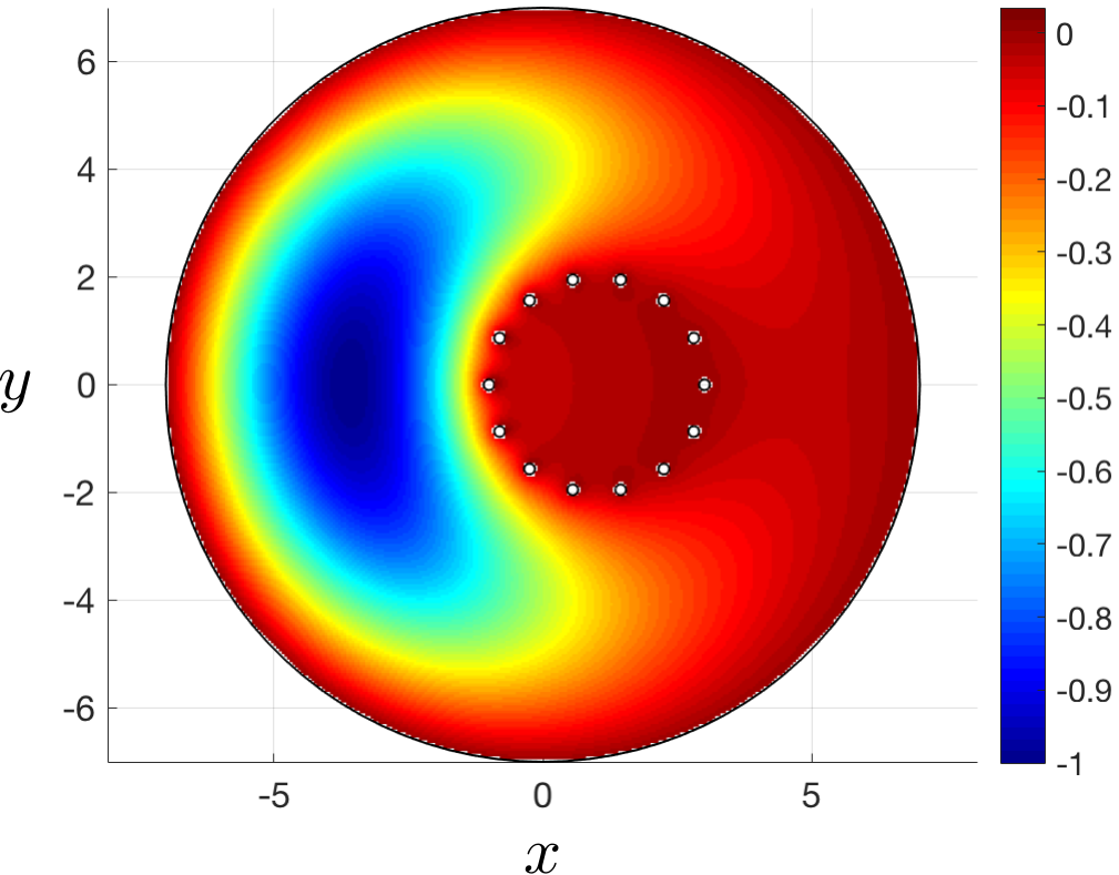
Figure 1: Cluster of small inclusions placed along a contour. The figure shows the eigenfunction corresponding to the first eigenvalue of the Dirichlet problem for the Laplacian, the eigenvalue is 0.308160.30816. The main region is the disk of radius R=7R=7 with the centre at the origin. Small circular rigid inclusions of radii r=0.1r=0.1 have their centres along the circle of radius 22 with the centre at (1,0)(1,0). The computation is produced in COMSOL.

For example, when a cluster of NN small circular inclusions of radius ε\varepsilon is assumed to be placed along a simple smooth closed curve in the plane we can use the method of meso-scale asymptotic approximations for solutions of scattering problems. When an incident wave of a radian frequency ω\omega is generated by a remote time-harmonic point source placed at y∈ℝ2{\textbf{y}}\in\mathbb{R}^{2} the approximation of the total field is constructed in the form

𝒢⁡(x,y,ω)∼G⁡(|x−y|,ω)+∑j=1Nβj​(y)​U(j)​(x),\mathcal{G}({\textbf{x}},{\textbf{y}},\omega)\sim G(|{\textbf{x}}-{\textbf{y}}|,\omega)+\sum_{j=1}^{N}\beta_{j}({\textbf{y}})U^{(j)}({\textbf{x}})\;,

where G⁡(|x−y|,ω)G(|{\textbf{x}}-{\textbf{y}}|,\omega) is Green’s function for the Helmholtz equation, U(j)U^{(j)} are special model fields associated with individual small inertial inclusions placed at O(j){\textbf{O}}^{(j)}, and βj\beta_{j} are the coefficients, found by solving an algebraic system of equations. The proof of the solvability of this algebraic system is similar to [1]. Compared to meso-scale two-dimensional clusters, this is a lower–dimensional case where inclusions are distributed along a contour. In addition to the above point-wise asymptotic approximation, the approach discussed here, can also be used to derive an effective transmission problem for the domain containing an inertial structured interface, and its solution provides a homogenisation approximation, which takes into account inertia of small inclusions. In particular, when small inclusions of mass mm form a periodic cluster of the overall mass MM distributed over a circle Γ\Gamma of unit radius, the coefficients βj\beta_{j} can be approximated by

βj​(y)=𝔊⁡(O(j),y),1≤j≤N,\beta_{j}({\textbf{y}})=\mathfrak{G}({\textbf{O}}^{(j)},{\textbf{y}})\;,\quad 1\leq j\leq N\;,

with the function 𝔊⁡(O(j),y)\mathfrak{G}({\textbf{O}}^{(j)},{\textbf{y}}) being the solution of the transmission problem for the following equation

μ​Δx​𝔊​(x,y)+ρ​ω2​𝔊​(x,y)+ℜ⁡(m,M,ω)​δ​(x−y)=0,\mu\Delta_{x}\mathfrak{G}({\textbf{x}},{\textbf{y}})+\rho\omega^{2}\mathfrak{G}({\textbf{x}},{\textbf{y}})+{\mathfrak{R}}(m,M,\omega)\delta({\textbf{x}}-{\textbf{y}})=0,

where μ\mu is the stiffness coefficient, ρ\rho is the mass density, and ℜ⁡(m,M,ω){\mathfrak{R}}(m,M,\omega) is the coefficient, that depends on the inertial properties of the cluster. While 𝔊⁡(O(j),y)\mathfrak{G}({\textbf{O}}^{(j)},{\textbf{y}}) satisfies the radiation condition at infinity, the transmission conditions across Γ\Gamma have the form

[𝔊⁡(x,y)]=0,[∂𝔊∂r​(x,y)]=−M2​π​m​αε​ℜ​(m,M,ω)​𝔊​(x,y).\big[\mathfrak{G}({\textbf{x}},{\textbf{y}})\big]=0\;,\quad\Big[\frac{\partial\mathfrak{G}}{\partial r}({\textbf{x}},{\textbf{y}})\Big]=-\frac{M}{2\pi m}\alpha_{\varepsilon}{\mathfrak{R}}(m,M,\omega)\mathfrak{G}({\textbf{x}},{\textbf{y}})\;.

Here αε=−4iμ/H0(1)(ρ/μωε),\alpha_{\varepsilon}=-4{\rm i\mu}/H^{(1)}_{0}(\sqrt{\rho/\mu}\omega{\varepsilon}), and H0(1)H^{(1)}_{0} is the Hankel function of the first kind.

For non-resonance forced problems, we also discuss solutions which can be interpreted as fields associated with the time-harmonic scattering from a lower-dimensional cluster of small inertial inclusions. The incident field is produced by a localised source, associated with a forced motion of one of rigid inclusions within the array, and formally the algorithm requires an asymptotic approximation of the harmonic capacitary potential in the low frequency regime. The approximation corresponds to a non-resonance case.

An example of a cluster of inclusions placed along a curve in a two-dimensional elastic membrane is shown in Fig. 1. Time-harmonic vibrations are considered here, and the inertia of small inclusions, as well as their size, separation and the size of the cluster represent parameters of the multi-scale asymptotic approximation.

We also analyse asymptotic solutions of an eigenvalue problem for a domain containing a lower-dimensional cluster of small inertial inclusions. Computations, discussed in the text, give a comparison between an analytical asymptotic procedure and a FEM simulation produced in COMSOL Multi-Physics shown in Fig. 1, with the analytical logarithmic asymptotic approximation shown in Fig. 2 and produce a remarkably good result.

The structure of the paper is as follows. In Section 2 we introduce the asymptotic model of a one-dimensional cluster of many inertial inclusions placed along a closed simple contour, which forms an inertial structured interface. Section 3 includes analysis of a low-frequency scattering in a finite elastic membrane with a sparse cluster of small movable rigid inclusions. The approximation of the first eigenvalue and the corresponding eigenfunction for a sparse or one-dimensional cluster of inertial inclusions in a finite elastic membrane is discussed in Section 4.

2 Elastic membrane with a one-dimensional cluster of inclusions

The problem considered concerns the scattering phenomena due to a cluster of NN inertial inclusions, Fε(j)F_{\varepsilon}^{(j)} with masses mjm_{j} and centres O(j){\textbf{O}}^{(j)}, 1≤j≤N1\leq j\leq N, in a membrane that has density ρ\rho and shear modulus μ\mu. Here ε\varepsilon is a small positive parameter, characterising the relative diameter of Fε(j)F_{\varepsilon}^{(j)}, similar to [2]. The overall mass of the cluster M=∑j=1NmjM=\sum_{j=1}^{N}m_{j} , is finite. Here we seek the asymptotic approximation of the solution of the scattering problem for a wave initiated by a point source positioned outside the cluster

μΔ𝒢(x,y,ω)+ρω2𝒢(x,y,ω)+δ(x−y)=0,x∈ℝ2\∪j=1NF¯ε(j),\mu\Delta\mathcal{G}({\textbf{x}},{\textbf{y}},\omega)+\rho\omega^{2}\mathcal{G}({\textbf{x}},{\textbf{y}},\omega)+\delta({\textbf{x}}-{\textbf{y}})=0\;,\quad{\textbf{x}}\in\mathbb{R}^{2}\backslash\cup_{j=1}^{N}{\overline{F}^{(j)}_{\varepsilon}}\;, (1)
𝒢⁡(x,y,ω)=Cj,x∈∂Fε(j),\mathcal{G}({\textbf{x}},{\textbf{y}},\omega)=C_{j}\;,\quad{\textbf{x}}\in\partial F^{(j)}_{\varepsilon}\;, (2)
∂𝒢∂rx​(x,y,ω)−i​k0​𝒢​(x,y,ω)=O⁡(1rx3/2), as rx→∞,\frac{\partial\mathcal{G}}{\partial r_{x}}({\textbf{x}},{\textbf{y}},\omega)-{\rm i}k_{0}\mathcal{G}({\textbf{x}},{\textbf{y}},\omega)=O\Big(\frac{1}{r_{x}^{3/2}}\Big)\;,\quad\text{ as }\quad r_{x}\to\infty\;, (3)

where the position of the point force is given by 𝐲∈ℝ2\∪j=1NF¯(j)ε{\bf y}\in\mathbb{R}^{2}\backslash\cup_{j=1}^{N}{\overline{F}^{(j)}_{\varepsilon}}, with y being separated by a finite distance from the cluster itself, rx=|x|r_{x}=|{\textbf{x}}| and CjC_{j} are constants that are determined in what follows. Here, ω\omega and k0=ρ​ω2/μk_{0}=\sqrt{{\rho\omega^{2}}/{\mu}} denote the radian frequency and wavenumber, respectively, of waves in the medium. In addition, as each mass vibrates in the membrane, the linear momentum balance for the mass is taken into account, imposing an additional condition in the form

−mj​ω2​Cj=μ​∫∂Fε(j)∂𝒢∂n​(x,y,ω)​d​sx,-m_{j}\omega^{2}C_{j}=\mu\int_{\partial F_{\varepsilon}^{(j)}}\frac{\partial{\cal G}}{\partial n}({\textbf{x}},{\textbf{y}},\omega)ds_{{\textbf{x}}}\;, (4)

for 1≤j≤N1\leq j\leq N, and n being the unit outward normal with respect to Fε(j)F_{\varepsilon}^{(j)}. This problem can be interpreted as that of the time-harmonic scattering of a wave produced by a point source in the presence of a cluster of small inertial inclusions positioned along a a simple smooth curve in a plane.

2.1 Model problems

We use the algorithm of the method of meso-scale asymptotic approximations [2] to formally construct an asymptotic approximation of the field 𝒢⁡(x,y,ω)\mathcal{G}({\textbf{x}},{\textbf{y}},\omega). The procedure requires several model problems.

2.1.1 Dynamic Green’s function

By GG we denote the dynamic Green’s function for the infinite membrane, that satisfies the equation

μ​Δ​G​(|x−y|,ω)+ρ​ω2​G​(|x−y|,ω)+δ⁡(x−y)=0,x,y∈ℝ2,\mu\Delta G(|{\textbf{x}}-{\textbf{y}}|,\omega)+\rho\omega^{2}G(|{\textbf{x}}-{\textbf{y}}|,\omega)+\delta({\textbf{x}}-{\textbf{y}})=0\;,\qquad{\textbf{x}},{\textbf{y}}\in\mathbb{R}^{2}\;, (5)

and the outgoing wave solution has the representation

G⁡(|x−y|,ω)=i4​μ​H0(1)​(k0​|x−y|),G(|{\textbf{x}}-{\textbf{y}}|,\omega)=\frac{{\rm i}}{4\mu}H^{(1)}_{0}\Big(k_{0}|{\textbf{x}}-{\textbf{y}}|\Big)\;, (6)

where k0=ρ​ω2/μk_{0}=\sqrt{{\rho\omega^{2}}/{\mu}}, and H0(1)H^{(1)}_{0} is the Hankel function of the first kind. In particular,

G⁡(|x−y|,ω)∼−12​π​μ​log⁡(k0​|x−y|),G(|{\textbf{x}}-{\textbf{y}}|,\omega)\sim-\frac{1}{2\pi\mu}\log(k_{0}|{\textbf{x}}-{\textbf{y}}|),

as k0​|x−y|→0.k_{0}|{\textbf{x}}-{\textbf{y}}|\to 0.

2.1.2 Dirichlet problem for the Helmholtz equation in the exterior of a finite inclusion

To allow for the correction of discrepancies on interior boundaries we introduce the problem

μ​Δ​U(j)​(x)+ρ​ω2​U(j)​(x)=0,x∈ℝ2\F¯ε(j),\mu\Delta U^{(j)}({\textbf{x}})+\rho\omega^{2}U^{(j)}({\textbf{x}})=0\;,\quad{\textbf{x}}\in\mathbb{R}^{2}\backslash{\overline{F}_{\varepsilon}^{(j)}}\;, (7)
U(j)​(x)=1,x∈∂Fε(j),U^{(j)}({\textbf{x}})=1\;,\quad{\textbf{x}}\in\partial F_{\varepsilon}^{(j)}\;, (8)

where the U(j)U^{(j)} also satisfies the radiation condition at infinity:

∂U(j)∂r​(x)−i​k0​U(j)​(x)=O⁡(1r3/2), as r→∞.\frac{\partial U^{(j)}}{\partial r}({\textbf{x}})-{\rm i}k_{0}U^{(j)}({\textbf{x}})=O(\frac{1}{r^{3/2}})\;,\quad\text{ as }\quad r\to\infty\;. (9)

2.2 Meso-scale approximation - formal asymptotics

The leading order approximation for the solution of (1)–(4) is sought in the form

𝒢⁡(x,y,ω)∼G⁡(|x−y|,ω)+∑j=1Nβj​(y)​U(j)​(x),\mathcal{G}({\textbf{x}},{\textbf{y}},\omega)\sim G(|{\textbf{x}}-{\textbf{y}}|,\omega)+\sum_{j=1}^{N}\beta_{j}({\textbf{y}})U^{(j)}({\textbf{x}})\;, (10)

where the coefficients βj\beta_{j} are to be determined.

2.2.1 The algebraic system

It follows from the boundary conditions (2) that to leading order we have

Ck=G⁡(|O(k)−y|,ω)+βk​(y)+∑j≠k1≤j≤Nβj​(y)​U(j)​(O(k)),x∈∂Fε(k),C_{k}={G}(|{\textbf{O}}^{(k)}-{\textbf{y}}|,\omega)+\beta_{k}({\textbf{y}})+\sum_{\begin{subarray}{c}j\neq k\\ 1\leq j\leq N\end{subarray}}\beta_{j}({\textbf{y}})U^{(j)}({{\textbf{O}}^{(k)}})\;,\quad{\textbf{x}}\in\partial F^{(k)}_{\varepsilon}\;, (11)

with 1≤k≤N1\leq k\leq N. Using the “equations of motions” (4) for individual inclusions together with (10), we deduce that the constants CkC_{k}, 1≤k≤N1\leq k\leq N, also satisfy the relations

−mk​ω2μ​Ck=∫∂Fε(k)∂𝒢⁡(x,y,ω)∂n​d​sx-\frac{m_{k}\omega^{2}}{\mu}C_{k}=\int_{\partial F_{\varepsilon}^{(k)}}\frac{\partial{\cal G}({\textbf{x}},{\textbf{y}},\omega)}{\partial n}ds_{x}
=\displaystyle= ∫∂Fε(k)∂G⁡(|x−y|,ω)∂n​d​sx+βk​(y)​∫∂Fε(k)∂U(k)​(x)∂n​d​sx\displaystyle\int_{\partial F_{\varepsilon}^{(k)}}\frac{\partial G(|{\textbf{x}}-{\textbf{y}}|,\omega)}{\partial n}ds_{x}+\beta_{k}({\textbf{y}})\int_{\partial F_{\varepsilon}^{(k)}}\frac{\partial U^{(k)}({\textbf{x}})}{\partial n}ds_{x} (12)
+\displaystyle+ ∑j≠k1≤j≤Nβj​(y)​∫∂Fε(k)∂U(j)​(x)∂n​d​sx,\displaystyle\sum_{\begin{subarray}{c}j\neq k\\ 1\leq j\leq N\end{subarray}}\beta_{j}({\textbf{y}})\int_{\partial F_{\varepsilon}^{(k)}}\frac{\partial U^{(j)}({\textbf{x}})}{\partial n}ds_{x},

where n stands for the unit outward normal on ∂Fε(j).\partial F_{\varepsilon}^{(j)}. Taking into account (5), (7), (8), and when j≠kj\neq k, using the integration by parts one can represent the boundary integrals in (12) via the integrals over Fε(j)F_{\varepsilon}^{(j)}, and hence the representation (12) takes the form

mk​ω2​Ck\displaystyle{m_{k}\omega^{2}}C_{k} =\displaystyle= −μβk(y)∫∂Fε(k)∂U(k)​(x)∂ndsx\displaystyle-\mu\beta_{k}({\textbf{y}})\int_{\partial F_{\varepsilon}^{(k)}}\frac{\partial U^{(k)}({\textbf{x}})}{\partial n}ds_{x} (13)
+\displaystyle+ ρ​ω2​∫Fε(k){G⁡(|x−y|,ω)+∑j≠k1≤j≤Nβj​(y)​U(j)​(x)}​𝑑x.\displaystyle{\rho\omega^{2}}\int_{F_{\varepsilon}^{(k)}}\Big\{G(|{\textbf{x}}-{\textbf{y}}|,\omega)+\sum_{\begin{subarray}{c}j\neq k\\ 1\leq j\leq N\end{subarray}}\beta_{j}({\textbf{y}})U^{(j)}({\textbf{x}})\Big\}d{\textbf{x}}.

Combining (11) and (13), we derive the algebraic system of equations for the coefficients βj,1≤j≤N,\beta_{j},~1\leq j\leq N, in the asymptotic approximation (10)

mk​ω2​G​(|O(k)−y|,ω)−ρ​ω2​∫Fε(k)G⁡(|x−y|,ω)​𝑑xm_{k}\omega^{2}G(|{\textbf{O}}^{(k)}-{\textbf{y}}|,\omega)-{\rho\omega^{2}}\int_{F_{\varepsilon}^{(k)}}G(|{\textbf{x}}-{\textbf{y}}|,\omega)d{\textbf{x}}
+βk​(y)​{mk​ω2+μ​∫∂Fε(k)∂U(k)​(x)∂n​d​sx}+\beta_{k}({\textbf{y}})\Big\{m_{k}\omega^{2}+\mu\int_{\partial F_{\varepsilon}^{(k)}}\frac{\partial U^{(k)}({\textbf{x}})}{\partial n}ds_{x}\Big\} (14)
+mkω2∑j≠k1≤j≤Nβj(y){U(j)(O(k))−ρmk∫Fε(k)U(j)(x)dx}=0.+m_{k}\omega^{2}\sum_{\begin{subarray}{c}j\neq k\\ 1\leq j\leq N\end{subarray}}\beta_{j}({\textbf{y}})\{U^{(j)}({{\textbf{O}}^{(k)}})-\frac{\rho}{m_{k}}\int_{F_{\varepsilon}^{(k)}}U^{(j)}({\textbf{x}})d{\textbf{x}}\}=0.

The justification of solvability of the above algebraic system for the coefficients βj\beta_{j} is similar to [1], and we do not discuss it here.

In particular, when inclusions Fε(j)F_{\varepsilon}^{(j)} are circular with radii ε​r(j)\varepsilon r^{(j)} and centres O(j){\textbf{O}}^{(j)}, where ε\varepsilon is a small non-dimensional parameter, we have

U(j)​(x)=αε(j)​G​(|x−O(j)|,ω),U^{(j)}({\textbf{x}})=\alpha^{(j)}_{\varepsilon}G(|{\textbf{x}}-{\textbf{O}}^{(j)}|,\omega)\;, (15)

where

αε(j)=−4​i​μH0(1)​(k0​ε​r(j)).\alpha^{(j)}_{\varepsilon}=-\frac{4{\rm i\mu}}{H^{(1)}_{0}\Big(k_{0}{\varepsilon}r^{(j)}\Big)}\;.

In this case, the algebraic system (14) for the coefficients βj\beta_{j}, 1≤j≤N1\leq j\leq N becomes

mk​G​(|O(k)−y|,ω)−ρ​∫Fε(k)G⁡(|x−y|,ω)​𝑑x\displaystyle m_{k}{G}(|{\textbf{O}}^{(k)}-{\textbf{y}}|,\omega)-{{{\rho}}\int_{F^{(k)}_{\varepsilon}}{G}(|{\textbf{x}}-{\textbf{y}}|,\omega)d{{\textbf{x}}}}
+βk​(mk+2​π​μ​ε​r(k)​αε(k)ω2​∂G⁡(r,ω)∂r|r=ε​r(k))\displaystyle+\beta_{k}\Big(m_{k}+\frac{2\pi{\mu}\varepsilon r^{(k)}\alpha_{\varepsilon}^{(k)}}{\omega^{2}}\frac{\partial G(r,\omega)}{\partial r}\Big|_{r=\varepsilon r^{(k)}}\Big)
+∑j≠k1≤j≤Nβjαε(j){mkG(|O(k)−O(j)|,ω)\displaystyle+\sum_{\begin{subarray}{c}j\neq k\\ 1\leq j\leq N\end{subarray}}\beta_{j}\alpha_{\varepsilon}^{(j)}\Big\{m_{k}G(|{\textbf{O}}^{(k)}-{\textbf{O}}^{(j)}|,\omega)
−ρ∫Fε(k)G(|x−O(j)|,ω)dx}=0.\displaystyle-{{\rho}\int_{F^{(k)}_{\varepsilon}}{G}(|{\textbf{x}}-{\textbf{O}}^{(j)}|,\omega)d{{\textbf{x}}}}\Big\}=0\;.
(16)

2.3 Scattering by a cluster of identical inclusions placed along a circular contour

Here, we assume that the circular inclusions Fε(j)F_{\varepsilon}^{(j)} have the same radii ε\varepsilon and mass mm and that their centres are uniformly distributed along the unit circular contour Γ1={x:|x|=1}\Gamma_{1}=\{{\textbf{x}}:|{\textbf{x}}|=1\}. Also, let d=2​π/Nd=2\pi/N, and assume that ε<Const​d3/2.\varepsilon<\mbox{Const}~d^{3/2}. We analyse the case when N→∞N\to\infty, while M=m​NM=mN is fixed, and obtain a problem concerning a membrane with an inertial ring.

When the inclusions Fε(k)F_{\varepsilon}^{(k)}, 1≤k≤N1\leq k\leq N, are all circular, some of the integrals appearing in (16) can be evaluated explicitly. In particular, when y is separated by a finite distance from the cluster of the inclusions, using the Graf’s addition theorem and expanding the Hankel function in a series we have:

H0(1)​(k0​|x−y|)=∑ν=−∞∞Hν(1)​(k0​|y−O(k)|)​Jν​(k0​|x−O(k)|)​ei​ν​(π−θk+θk,y).H_{0}^{(1)}(k_{0}|{\textbf{x}}-{\textbf{y}}|)=\sum_{\nu=-\infty}^{\infty}H_{\nu}^{(1)}(k_{0}|{\textbf{y}}-{\textbf{O}}^{(k)}|)J_{\nu}(k_{0}|{\textbf{x}}-{\textbf{O}}^{(k)}|)e^{{\rm i}\nu(\pi-\theta_{k}+\theta_{k,{\textbf{y}}})}\;.

where θk\theta_{k} is the polar angle of x measured with respect to O(k){\textbf{O}}^{(k)} and θk,y\theta_{k,{\textbf{y}}} is the polar angle of O(k){\textbf{O}}^{(k)} measured with respect to y. Hence, as ε→0,\varepsilon\to 0,

∫Fε(k)G⁡(|x−y|,ω)​d​sx\displaystyle\int_{F_{\varepsilon}^{(k)}}G(|{\textbf{x}}-{\textbf{y}}|,\omega)ds_{{\textbf{x}}} =\displaystyle= π​ε2​G​(|O(k)−y|,ω)+O⁡(ε3)=O⁡(ε2),\displaystyle\pi\varepsilon^{2}G(|{\textbf{O}}^{(k)}-{\textbf{y}}|,\omega)+O(\varepsilon^{3})=O(\varepsilon^{2}),

and for j≠kj\neq k, it is derived that

∫Fε(k)G⁡(|x−O(j)|,ω)​d​sx\displaystyle\int_{F_{\varepsilon}^{(k)}}G(|{\textbf{x}}-{\textbf{O}}^{(j)}|,\omega)ds_{{\textbf{x}}} =\displaystyle= π​ε2​G​(|O(k)−O(j)|,ω)\displaystyle\pi\varepsilon^{2}G(|{\textbf{O}}^{(k)}-{\textbf{O}}^{(j)}|,\omega)
+O⁡(ε3/d)=O⁡(ε2​|log⁡d|).+O(\varepsilon^{3}/d)=O(\varepsilon^{2}|\log d|).

We also note that

2​π​ε​μ​r(k)​∂G∂r​(r,ω)|r=ε​r(k)=−1+O⁡(ε2​|log⁡ε|).{2\pi\varepsilon\mu r^{(k)}}\frac{\partial G}{\partial r}(r,\omega)\Big|_{r=\varepsilon r^{(k)}}=-1+O(\varepsilon^{2}|\log\varepsilon|).

For the cluster of identical inclusions, the system (16), to leading order, becomes

m​G​(|O(k)−y|,ω)+βk​(y)​(m−αεω2)\displaystyle m{G}(|{\textbf{O}}^{(k)}-{\textbf{y}}|,\omega)+\beta_{k}({\textbf{y}})\Big(m-\frac{\alpha_{\varepsilon}}{\omega^{2}}\Big)
+mαε∑j≠k1≤j≤Nβj(y)G(|O(k)−O(j)|)=0,\displaystyle+m\alpha_{\varepsilon}\sum_{\begin{subarray}{c}j\neq k\\ 1\leq j\leq N\end{subarray}}\beta_{j}({\textbf{y}})G(|{\textbf{O}}^{(k)}-{\textbf{O}}^{(j)}|)=0\;,
(17)

where 1≤k≤N,1\leq k\leq N, and

αε=−4​i​μH0(1)​(k0​ε).\alpha_{\varepsilon}=-\frac{4{\rm i\mu}}{H^{(1)}_{0}\Big(k_{0}{\varepsilon}\Big)}\;.

2.4 Derivation of the transmission conditions for 𝔊\mathfrak{G} in the auxiliary problem

Assume that positions of the centres of inclusions Fε(j)F^{(j)}_{\varepsilon} are

O(j)=(cos⁡(2​π​(j−1)/N),sin⁡(2​π​(j−1)/N))T,1≤j≤N,{\textbf{O}}^{(j)}=(\cos(2\pi(j-1)/N),\sin(2\pi(j-1)/N))^{\rm T}\;,\qquad 1\leq j\leq N\;,

and let 𝔊⁡(x,y)\mathfrak{G}({\textbf{x}},{\textbf{y}}) be a function such that

βj​(y)=𝔊⁡(O(j),y),1≤j≤N.\beta_{j}({\textbf{y}})=\mathfrak{G}({\textbf{O}}^{(j)},{\textbf{y}})\;,\quad 1\leq j\leq N\;. (18)

Equations (17) can be re-written in the form

m​G​(|O(k)−y|,ω)+βk​(y)​(m−αεω2)\displaystyle m{G}(|{\textbf{O}}^{(k)}-{\textbf{y}}|,\omega)+\beta_{k}({\textbf{y}})\Big(m-\frac{\alpha_{\varepsilon}}{\omega^{2}}\Big)
+M​αε2​π∑j≠k1≤j≤Nβj(y)G(|O(k)−O(j)|)2​πN=0.\displaystyle+\frac{M\alpha_{\varepsilon}}{2\pi}\sum_{\begin{subarray}{c}j\neq k\\ 1\leq j\leq N\end{subarray}}\beta_{j}({\textbf{y}})G(|{\textbf{O}}^{(k)}-{\textbf{O}}^{(j)}|)\frac{2\pi}{N}=0\;. (19)

By considering the sum in (19) as the Riemann sum and taking the limit as N→∞N\to\infty, we arrive at

m​ω2​G​(|x−y|,ω)+𝔊⁡(x,y)​(m​ω2−αε)m\omega^{2}{G}(|{\textbf{x}}-{\textbf{y}}|,\omega)+\mathfrak{G}({\textbf{x}},{\textbf{y}})(m\omega^{2}-\alpha_{\varepsilon})
+M​ω2​αε2​π∫02​πG(|x−𝜼|,ω)𝔊(𝜼,y)dθ𝜼=0.+\frac{M\omega^{2}\alpha_{\varepsilon}}{2\pi}\int_{0}^{2\pi}G(|{\textbf{x}}-\mbox{\boldmath${\eta}$}|,\omega)\mathfrak{G}(\mbox{\boldmath${\eta}$},{\textbf{y}})d\theta_{\scriptsize{\mbox{\boldmath${\eta}$}}}=0\;. (20)

When this equation is extended to x outside Γ1\Gamma_{1}, one can apply the Laplacian in x, use (5) and derive

0=−m​ω2​(ρ​ω2μ​G​(|x−y|,ω)+1μ​δ​(x−y))+(m​ω2−αε)​Δx​𝔊​(x,y)0=-m\omega^{2}(\frac{\rho\omega^{2}}{\mu}G(|{\textbf{x}}-{\textbf{y}}|,\omega)+\frac{1}{\mu}\delta({\textbf{x}}-{\textbf{y}}))+(m\omega^{2}-\alpha_{\varepsilon})\Delta_{x}\mathfrak{G}({\textbf{x}},{\textbf{y}})
−M​ω4​αε​ρ2​π​μ∫Γ1G(|x−𝜼|,ω)𝔊(𝜼,y)dθ𝜼.-\frac{M\omega^{4}\alpha_{\varepsilon}\rho}{2\pi\mu}\int_{\Gamma_{1}}G(|{\textbf{x}}-\mbox{\boldmath${\eta}$}|,\omega)\mathfrak{G}(\mbox{\boldmath${\eta}$},{\textbf{y}})d\theta_{\scriptsize{\mbox{\boldmath${\eta}$}}}. (21)

Furthermore, using (20) and (21) we obtain the equation for 𝔊⁡(x,y)\mathfrak{G}({\textbf{x}},{\textbf{y}}) in the form

μ​Δx​𝔊​(x,y)+ρ​ω2​𝔊​(x,y)+m​ω2αε−m​ω2​δ​(x−y)=0.\mu\Delta_{x}\mathfrak{G}({\textbf{x}},{\textbf{y}})+\rho\omega^{2}\mathfrak{G}({\textbf{x}},{\textbf{y}})+\frac{m\omega^{2}}{\alpha_{\varepsilon}-m\omega^{2}}\delta({\textbf{x}}-{\textbf{y}})=0. (22)

We note that |αε|=O⁡(|log⁡ε|−1)|\alpha_{\varepsilon}|=O(|\log\varepsilon|^{-1}), with mm being of order O⁡(d)O(d), and the radian frequency ω2\omega^{2} serving as an additional control parameter.

In addition, we take the normal derivative in (20) and use the following relations when x∈Γ1{\textbf{x}}\in\Gamma_{1}

lim𝝃→Γ1±∫Γ1∂G∂r​(|𝝃−𝜼|,ω)​𝔊​(𝜼,y)​d​s𝜼=∓12​𝔊​(x,y)+∫Γ1∂G∂r​(|x−𝜼|,ω)​𝔊​(𝜼,y)​d​s𝜼,\lim_{\scriptsize{\mbox{\boldmath${\xi}$}}\to\Gamma_{1}^{\pm}}\int_{\Gamma_{1}}\frac{\partial G}{\partial r}(|\mbox{\boldmath${\xi}$}-\mbox{\boldmath${\eta}$}|,\omega)\mathfrak{G}(\mbox{\boldmath${\eta}$},{\textbf{y}})ds_{\mbox{\boldmath${\eta}$}}=\mp\frac{1}{2}\mathfrak{G}({\textbf{x}},{\textbf{y}})+\int_{\Gamma_{1}}\frac{\partial G}{\partial r}(|{\textbf{x}}-\mbox{\boldmath${\eta}$}|,\omega)\mathfrak{G}(\mbox{\boldmath${\eta}$},{\textbf{y}})ds_{\scriptsize{\mbox{\boldmath${\eta}$}}}\;,\quad

(see [13]), and obtain the transmission condition across Γ1\Gamma_{1}

[𝔊⁡(x,y)]=0,[∂𝔊∂r​(x,y)]=M​ω2​αε2​π​(m​ω2−αε)​𝔊​(x,y),\big[\mathfrak{G}({\textbf{x}},{\textbf{y}})\big]=0\;,\quad\Big[\frac{\partial\mathfrak{G}}{\partial r}({\textbf{x}},{\textbf{y}})\Big]=\frac{M\omega^{2}\alpha_{\varepsilon}}{2\pi(m\omega^{2}-\alpha_{\varepsilon})}\mathfrak{G}({\textbf{x}},{\textbf{y}})\;, (23)

with [𝔊⁡(x,y)]\big[\mathfrak{G}({\textbf{x}},{\textbf{y}})\big] denoting the jump of 𝔊⁡(x,y)\mathfrak{G}({\textbf{x}},{\textbf{y}}) across Γ1\Gamma_{1}, while the point y is separated by a finite distance from Γ1\Gamma_{1}:

[𝔊⁡(x,y)]=𝔊⁡(x,y)|x∈Γ1+−𝔊⁡(x,y)|x∈Γ1−.\big[\mathfrak{G}({\textbf{x}},{\textbf{y}})\big]=\mathfrak{G}({\textbf{x}},{\textbf{y}})\Big|_{{\textbf{x}}\in\Gamma_{1}^{+}}-\mathfrak{G}({\textbf{x}},{\textbf{y}})\Big|_{{\textbf{x}}\in\Gamma_{1}^{-}}\;.

Thus, the function 𝔊⁡(x,y)\mathfrak{G}({\textbf{x}},{\textbf{y}}) can be defined as a solution of (22), (23), subject to the radiation condition at infinity. This provides an alternative homogenisation approximation (18) for the coefficients βj\beta_{j} in (10), which takes into account the inertial transmission conditions across the structured interface formed by a cluster of small inclusions.

3 Low-frequency scattering in a finite elastic membrane with a sparse cluster of small movable rigid inclusions

Consider a finite elastic membrane Ω⊂ℝ2\Omega\subset\mathbb{R}^{2}, together with a finite sparse cluster of small rigid inclusions Fε(j)⊂Ω,j=1,…,N,F_{\varepsilon}^{(j)}\subset\Omega,~j=1,\ldots,N, of zero mass density, containing interior points O(j){\textbf{O}}^{(j)}. It is assumed that the small inclusions Fε(j),j=1,…,N,F_{\varepsilon}^{(j)},j=1,\ldots,N, are separated by the finite distance from the exterior boundary ∂Ω.\partial\Omega. We use the notation

ΩN=Ω∖∪j=1NF¯ε(j).\Omega_{N}=\Omega\setminus\cup_{j=1}^{N}\overline{F}_{\varepsilon}^{(j)}.

Given the mass density ρ\rho and a time-harmonic vibration of small radian frequency ω,\omega, applied to the inclusion Fε(1)F_{\varepsilon}^{(1)}, the amplitude of the out-of-plane displacement satisfies the problem:

μ​Δ​u​(x)+ρ​ω2​u​(x)\displaystyle\mu\Delta u({\textbf{x}})+\rho\omega^{2}u({\textbf{x}}) =\displaystyle= 0,x∈ΩN\displaystyle 0,~~{\textbf{x}}\in\Omega_{N} (24)
u⁡(x)\displaystyle u({\textbf{x}}) =\displaystyle= 1,x∈∂Fε(1)\displaystyle 1,~~{\textbf{x}}\in\partial F_{\varepsilon}^{(1)} (25)
u⁡(x)\displaystyle u({\textbf{x}}) =\displaystyle= Aj,x∈∂Fε(j)​1<j≤N,\displaystyle A_{j},~{\textbf{x}}\in\partial F_{\varepsilon}^{(j)}~1<j\leq N, (26)
u⁡(x)\displaystyle u({\textbf{x}}) =\displaystyle= 0,x∈∂Ω\displaystyle 0,~~{\textbf{x}}\in\partial\Omega (27)

where

∫∂Fε(j)∂u∂n​𝑑s=0,1<j≤N.\int_{\partial F_{\varepsilon}^{(j)}}\frac{\partial u}{\partial n}ds=0,~~1<j\leq N. (28)

The constants AjA_{j} are to be determined, and it is assumed that small inclusions Fε(j)F_{\varepsilon}^{(j)} are separated by a finite distance. We introduce a small non-dimensional parameter ff, with ε<f\varepsilon<f, in such a way that ρ​ω2=f​λ\rho\omega^{2}=f\lambda. Here, we use the normalisation μ=1\mu=1, and hence the equation (24) takes the form

Δ​u​(x)+f​λ​u​(x)=0,x∈ΩN.\Delta u({\textbf{x}})+f\lambda u({\textbf{x}})=0,~~{\textbf{x}}\in\Omega_{N}. (29)

Also, the notation F(j)F^{(j)} is used for scaled inclusions, such that F(j)={x:ε​x+O(j)∈Fε(j)}.F^{(j)}=\{{\textbf{x}}:\varepsilon{\textbf{x}}+{\textbf{O}}^{(j)}\in F^{(j)}_{\varepsilon}\}.

3.1 Green’s function and the relative capacitary potential

We use the result of [2] and employ the relative capacitary potential Pε(1)​(x)P_{\varepsilon}^{(1)}({\textbf{x}}), which satisfies the boundary value problem in Ω∖F¯ε(1)\Omega\setminus\overline{F}_{\varepsilon}^{(1)}

Δ​Pε(1)​(x)\displaystyle\Delta P_{\varepsilon}^{(1)}({\textbf{x}}) =\displaystyle= 0,x∈Ω∖F¯ε(1),\displaystyle 0,~~{\textbf{x}}\in\Omega\setminus\overline{F}_{\varepsilon}^{(1)}, (30)
Pε(1)​(x)\displaystyle P_{\varepsilon}^{(1)}({\textbf{x}}) =\displaystyle= 1,x∈∂Fε(1),\displaystyle 1,~~{\textbf{x}}\in\partial F_{\varepsilon}^{(1)}, (31)
Pε(1)​(x)\displaystyle P_{\varepsilon}^{(1)}({\textbf{x}}) =\displaystyle= 0,x∈∂Ω.\displaystyle 0,~~{\textbf{x}}\in\partial\Omega. (32)

The notations G⁡(x,y)G({\textbf{x}},{\textbf{y}}) and g⁡(x,y)g({\textbf{x}},{\textbf{y}}) are used for Green’s functions in Ω\Omega and ℝ2∖F¯(1)\mathbb{R}^{2}\setminus\overline{F}^{(1)}, respectively. Thus,

Δ​G​(x,y)+δ⁡(x−y)\displaystyle\Delta G({\textbf{x}},{\textbf{y}})+\delta({\textbf{x}}-{\textbf{y}}) =\displaystyle= 0,x,y∈Ω,\displaystyle 0,~~{\textbf{x}},{\textbf{y}}\in\Omega, (33)
G⁡(x,y)\displaystyle G({\textbf{x}},{\textbf{y}}) =\displaystyle= 0,x∈∂Ω,y∈Ω,\displaystyle 0,~~{\textbf{x}}\in\partial\Omega,~{\textbf{y}}\in\Omega, (34)

and

Δ​g​(𝝃,𝜼)+δ⁡(𝝃−𝜼)\displaystyle\Delta g(\mbox{\boldmath${\xi}$},\mbox{\boldmath${\eta}$})+\delta(\mbox{\boldmath${\xi}$}-\mbox{\boldmath${\eta}$}) =\displaystyle= 0,𝝃,𝜼∈ℝ2∖F¯(1),\displaystyle 0,~~\mbox{\boldmath${\xi}$},\mbox{\boldmath${\eta}$}\in\mathbb{R}^{2}\setminus\overline{F}^{(1)}, (35)
g⁡(𝝃,𝜼)\displaystyle g(\mbox{\boldmath${\xi}$},\mbox{\boldmath${\eta}$}) =\displaystyle= 0,𝝃∈∂F(1),𝜼∈ℝ2∖F¯(1),\displaystyle 0,~~\mbox{\boldmath${\xi}$}\in\partial F^{(1)},\mbox{\boldmath${\eta}$}\in\mathbb{R}^{2}\setminus\overline{F}^{(1)}, (36)
g⁡(𝝃,𝜼)​is bounded\displaystyle g(\mbox{\boldmath${\xi}$},\mbox{\boldmath${\eta}$})~\mbox{is bounded} as |𝝃|→∞​and​𝜼∈ℝ2∖F¯(1).\displaystyle|\mbox{\boldmath${\xi}$}|\to\infty~\mbox{and}~\mbox{\boldmath${\eta}$}\in\mathbb{R}^{2}\setminus\overline{F}^{(1)}. (37)

According to Lemma 1.4 in [2], the relative capacitary potential Pε(1)P_{\varepsilon}^{(1)} has the asymptotic representation

Pε(1)​(x)=−G⁡(x,O(1))+ζ⁡(x−O(1)ε)−12​π​log⁡|x−O(1)|ε​rF12​π​log⁡ε​rFRΩ+pε​(x),P_{\varepsilon}^{(1)}({\textbf{x}})=\frac{-G({\textbf{x}},{\textbf{O}}^{(1)})+\zeta(\frac{{\textbf{x}}-{\textbf{O}}^{(1)}}{\varepsilon})-\frac{1}{2\pi}\log\frac{|{\textbf{x}}-{\textbf{O}}^{(1)}|}{\varepsilon r_{F}}}{\frac{1}{2\pi}\log\frac{\varepsilon r_{F}}{R_{\Omega}}}+p_{\varepsilon}({\textbf{x}}), (38)

where pε​(x)=O⁡(ε​|log⁡ε|−1)p_{\varepsilon}({\textbf{x}})=O(\varepsilon|\log\varepsilon|^{-1}) uniformly with respect to x∈Ω∖F¯ε(1){\textbf{x}}\in\Omega\setminus\overline{F}_{\varepsilon}^{(1)}. In the above formula (38), the notations rFr_{F} and RΩR_{\Omega} stand for the inner conformal radius of F(1)F^{(1)} with respect to O(1){\textbf{O}}^{(1)}, and the outer conformal radius of Ω\Omega relative to O(1){\textbf{O}}^{(1)}, respectively, as discussed in Section 1.2.1 of [2]. The function ζ\zeta is defined by

ζ⁡(𝜼)=lim|𝝃|→∞g⁡(𝝃,𝜼).\zeta(\mbox{\boldmath${\eta}$})=\lim_{|\mbox{\boldmath${\xi}$}|\to\infty}g(\mbox{\boldmath${\xi}$},\mbox{\boldmath${\eta}$}). (39)

In particular, for the case when the inclusion Fε(1)F_{\varepsilon}^{(1)} is circular of radius ε​rF\varepsilon r_{F}, the formula (38) simplifies as

Pε(1)​(x)=𝔅1​G​(x,O(1))+O⁡(ε),𝔅1=−(12​π​log⁡ε​rF+H⁡(O(1),O(1)))−1,P_{\varepsilon}^{(1)}({\textbf{x}})={\mathfrak{B}}_{1}G({\textbf{x}},{\textbf{O}}^{(1)})+O(\varepsilon),~~{\mathfrak{B}}_{1}=-(\frac{1}{2\pi}\log{\varepsilon r_{F}}+H({\textbf{O}}^{(1)},{\textbf{O}}^{(1)}))^{-1}, (40)

where the regular part H⁡(x,y)H({\textbf{x}},{\textbf{y}}) of Green’s function GG is a harmonic function defined by

H⁡(x,y)=12​π​log⁡|x−y|−1−G⁡(x,y).H({\textbf{x}},{\textbf{y}})=\frac{1}{2\pi}\log|{\textbf{x}}-{\textbf{y}}|^{-1}-G({\textbf{x}},{\textbf{y}}). (41)

3.2 Formal asymptotic approximation

The asymptotic approximation is sought in the form

u⁡(x)∼Pε(1)​(x)+f​u(2)​(x),u({\textbf{x}})\sim P^{(1)}_{\varepsilon}({\textbf{x}})+fu^{(2)}({\textbf{x}}), (42)

and, owing to (26), the constants Aj,j=2,…,N,A_{j},~j=2,\ldots,N, representing the rigid motion displacements of massless inclusions, are

Aj∼Pε(1)​(O(j))+f​Aj(2),A_{j}\sim P_{\varepsilon}^{(1)}({\textbf{O}}^{(j)})+fA_{j}^{(2)}, (43)

whereas u(2)u^{(2)} satisfies the boundary value problem

Δ​u(2)​(x)+λ​Pε(1)​(x)\displaystyle\Delta u^{(2)}({\textbf{x}})+\lambda P^{(1)}_{\varepsilon}({\textbf{x}}) =\displaystyle= 0​in​ΩN,\displaystyle 0~~\mbox{in}~\Omega_{N}, (44)
u(2)​(x)\displaystyle u^{(2)}({\textbf{x}}) =\displaystyle= 0,x∈∂Fε(1),\displaystyle 0,~{\textbf{x}}\in\partial F_{\varepsilon}^{(1)}, (45)
u(2)​(x)\displaystyle u^{(2)}({\textbf{x}}) =\displaystyle= Aj(2),x∈∂Fε(j),j=2,…,N,\displaystyle A^{(2)}_{j},~{\textbf{x}}\in\partial F_{\varepsilon}^{(j)},j=2,\ldots,N, (46)
u(2)​(x)\displaystyle u^{(2)}({\textbf{x}}) =\displaystyle= 0,x∈∂Ω.\displaystyle 0,~{\textbf{x}}\in\partial\Omega. (47)

By assuming a circular shape of the inclusion Fε(1)F_{\varepsilon}^{(1)}, using formula (40), and introducing an auxiliary problem

Δ​V​(x)+λ​𝔅1​G​(x,O(1))\displaystyle\Delta V({\textbf{x}})+\lambda{\mathfrak{B}}_{1}G({\textbf{x}},{\textbf{O}}^{(1)}) =\displaystyle= 0​in​Ω,\displaystyle 0~~\mbox{in}~\Omega, (48)
V⁡(x)\displaystyle V({\textbf{x}}) =\displaystyle= 0,x∈∂Ω,\displaystyle 0,~{\textbf{x}}\in\partial\Omega, (49)

we deduce

V⁡(x)=λ​𝔅1​∫ΩG⁡(z,x)​G​(z,O(1))​𝑑z,V({\textbf{x}})=\lambda{\mathfrak{B}}_{1}\int_{\Omega}G({\textbf{z}},{\textbf{x}})G({\textbf{z}},{\textbf{O}}^{(1)})d{\textbf{z}}, (50)

and

Aj(2)=V⁡(O(j))−V⁡(O(1))​Pε(1)​(O(j)).A^{(2)}_{j}=V({\textbf{O}}^{(j)})-V({\textbf{O}}^{(1)})P_{\varepsilon}^{(1)}({\textbf{O}}^{(j)}). (51)

In this case, the approximation (42) can be rewritten in the form

u⁡(x)=Pε(1)​(x)+f⁡(V⁡(x)−V⁡(O(1))​Pε(1)​(x))+𝔯⁡(x),u({\textbf{x}})=P^{(1)}_{\varepsilon}({\textbf{x}})+f(V({\textbf{x}})-V({\textbf{O}}^{(1)})P^{(1)}_{\varepsilon}({\textbf{x}}))+{\mathfrak{r}}({\textbf{x}}), (52)

where the remainder term satisfies the problem

Δ​𝔯​(x)+f​λ​𝔯​(x)\displaystyle\Delta{\mathfrak{r}}({\textbf{x}})+f\lambda{\mathfrak{r}}({\textbf{x}}) =\displaystyle= −f​λ​(Pε(1)​(x)−𝔅1​G​(x,O(1)))\displaystyle-f\lambda(P_{\varepsilon}^{(1)}({\textbf{x}})-{\mathfrak{B}}_{1}G({\textbf{x}},{\textbf{O}}^{(1)})) (53)
−\displaystyle- f2​λ​(V⁡(x)−V⁡(O(1))​Pε(1)​(x)),\displaystyle f^{2}\lambda(V({\textbf{x}})-V({\textbf{O}}^{(1)})P_{\varepsilon}^{(1)}({\textbf{x}})),
𝔯⁡(x)\displaystyle{\mathfrak{r}}({\textbf{x}}) =\displaystyle= 0​on​∂Ω,\displaystyle 0~~\mbox{on}~\partial\Omega, (54)
𝔯⁡(x)\displaystyle{\mathfrak{r}}({\textbf{x}}) =\displaystyle= −f(V(x)−V(O(1)))on∂Fε(1),\displaystyle-f(V({\textbf{x}})-V({\textbf{O}}^{(1)}))~~\mbox{on}~\partial F_{\varepsilon}^{(1)}, (55)
𝔯⁡(x)\displaystyle{\mathfrak{r}}({\textbf{x}}) =\displaystyle= Aj−Pε(1)​(x)−f⁡(V⁡(x)−V⁡(O(1))​Pε(1)​(x))\displaystyle A_{j}-P_{\varepsilon}^{(1)}({\textbf{x}})-f(V({\textbf{x}})-V({\textbf{O}}^{(1)})P_{\varepsilon}^{(1)}({\textbf{x}})) (56)
on​∂Fε(j),j=2,…,N.\displaystyle~~\mbox{on}~\partial F_{\varepsilon}^{(j)},~j=2,\ldots,N.

For the case when the inclusion Fε(1)F_{\varepsilon}^{(1)} is circular, taking into account that the small quantity f​λf\lambda is separated from the spectrum, and using the formulae (43), (51) and (52) we deduce that

𝔯⁡(x)=O⁡(f​ε){\mathfrak{r}}({\textbf{x}})=O(f\varepsilon) (57)

when x is outside a neighbourhood of the cluster of small inclusions, and

𝔯⁡(x)=O⁡(max⁡{f​ε​|log⁡ε|,ε}){\mathfrak{r}}({\textbf{x}})=O({\rm max}\{f\varepsilon|\log\varepsilon|,~\varepsilon\}) (58)

when x is in the vicinity of the cluster of small inclusions.

The idea of the proof for the case of a sparse cluster of small circular inclusions is based on the representation of the solution 𝔯{\mathfrak{r}} of (53)–(56) as a sum of integrals over ΩN\Omega_{N} and the boundaries of Fε(j)F_{\varepsilon}^{(j)} :

𝔯(x)=−∫ΩNℱ(y)gΩ(x,y)dy{\mathfrak{r}}({\textbf{x}})=-\int_{\Omega_{N}}{\cal F}({\textbf{y}})g_{\Omega}({\textbf{x}},{\textbf{y}})d{\textbf{y}}
+∑j=1N∫∂Fε(j){gΩ(x,y)∂𝔯∂ny(y)−Φj(y)∂gΩ∂ny(x,y)}dsy+\sum_{j=1}^{N}\int_{\partial F_{\varepsilon}^{(j)}}\Big\{g_{\Omega}({\textbf{x}},{\textbf{y}})\frac{\partial{\mathfrak{r}}}{\partial n_{\textbf{y}}}({\textbf{y}})-\Phi_{j}({\textbf{y}})\frac{\partial g_{\Omega}}{\partial n_{\textbf{y}}}({\textbf{x}},{\textbf{y}})\Big\}ds_{\textbf{y}}

where ℱ{\cal F} is the right-hand side in (53), n is the unit outward normal with respect to ΩN\Omega_{N}, and the functions Φj\Phi_{j} are the right-hand sides in (55) for j=1j=1, and in (56) for 2≤j≤N.2\leq j\leq N. Here gΩ​(x,y)g_{\Omega}({\textbf{x}},{\textbf{y}}) is Green’s function for the Helmholtz equation in the unperturbed domain Ω\Omega:

Δx​gΩ​(x,y)+k2​gΩ​(x,y)+δ⁡(x−y)=0,x,y∈Ω,\Delta_{\textbf{x}}g_{\Omega}({\textbf{x}},{\textbf{y}})+k^{2}g_{\Omega}({\textbf{x}},{\textbf{y}})+\delta({\textbf{x}}-{\textbf{y}})=0,~{\textbf{x}},{\textbf{y}}\in\Omega,
gΩ​(x,y)=0,when​x∈∂Ω,y∈Ω,g_{\Omega}({\textbf{x}},{\textbf{y}})=0,~\mbox{when}~{\textbf{x}}\in\partial\Omega,~{\textbf{y}}\in\Omega,

where k=f​λ.k=\sqrt{f\lambda}. We also note that the flux of 𝔯{\mathfrak{r}} over the boundaries of small inclusions is not zero, i.e.

∫Fε(1)∂𝔯∂ndx=O(f),∫Fε(j)∂𝔯∂ndx=O(fε2),j=2,…,N.\int_{F_{\varepsilon}^{(1)}}\frac{\partial{\mathfrak{r}}}{\partial n}d{\textbf{x}}=O(f),~\int_{F_{\varepsilon}^{(j)}}\frac{\partial{\mathfrak{r}}}{\partial n}d{\textbf{x}}=O(f\varepsilon^{2}),~j=2,\ldots,N.

By considering three cases for 𝔯⁡(x){\mathfrak{r}}({\textbf{x}}), (a) x is outside the neighbourhood of the sparse cluster of small circular inclusions, (b) x is in the vicinity of Fε(1)F_{\varepsilon}^{(1)}, and (c) x is in the vicinity of Fε(j),j=2,…,NF_{\varepsilon}^{(j)},~j=2,\ldots,N, we deduce (57) and (58).

4 The first positive eigenvalue for a lower– dimensional cluster of inertial inclusions in a finite elastic membrane

Section 3 has addressed low frequency non-resonance vibrations for a sparse cluster of massless inclusions (each individual inclusion has zero inertia). In this case, Green’s function for the Laplacian is used as one of the model solutions. If the small inclusions have a non-zero inertia the problem requires Green’s function for the Helmholtz operator, which takes into account time-harmonic vibrations of the multi-scale system. In this section, we consider the eigenvalue problem for a finite membrane Ω⊂ℝ2\Omega\subset\mathbb{R}^{2}, and contained in this membrane is a sparse or lower-dimensional cluster of small inertial inclusions Fε(j)F_{\varepsilon}^{(j)} of the mass mjm_{j}, 1≤j≤N1\leq j\leq N . In this case, if dd is the minimum distance between two neighbouring inclusions within the cluster, we assume that d​N=O⁡(1).dN=O(1). As before, we use the notation ΩN:=Ω\∪j=1NF¯(j)ε\Omega_{N}:=\Omega\backslash\cup_{j=1}^{N}{\overline{F}^{(j)}_{\varepsilon}}. The eigenfunction uNu_{N} and the corresponding eigenvalue λN\lambda_{N} are defined as the solution of the problem

Δ​uN​(x)+λN​uN​(x)=0,x∈ΩN,\Delta u_{N}({\textbf{x}})+\lambda_{N}u_{N}({\textbf{x}})=0\;,\quad{\textbf{x}}\in\Omega_{N}\;, (59)
uN​(x)=0,x∈∂Ω,u_{N}({\textbf{x}})=0\;,\quad{\textbf{x}}\in\partial\Omega, (60)
uN​(x)=Aj,x∈∂Fε(j),u_{N}({\textbf{x}})=A_{j}\;,\quad{\textbf{x}}\in\partial F^{(j)}_{\varepsilon}\;, (61)

with

−γj​λN​Aj=∫∂Fε(j)∂uN​(x)∂n​𝑑s,x∈∂Fε(j).-\gamma_{j}\lambda_{N}A_{j}=\int_{\partial F_{\varepsilon}^{(j)}}\frac{\partial u_{N}({\textbf{x}})}{\partial n}ds\;,\quad{\textbf{x}}\in\partial F^{(j)}_{\varepsilon}\;. (62)

where λN=ρ​ω2/μ\lambda_{N}=\rho\omega^{2}/\mu and γj=mjρ\gamma_{j}=\frac{m_{j}}{\rho}, 1≤j≤N1\leq j\leq N, and nn is the unit outward normal with respect to Fε(j)F^{(j)}_{\varepsilon}. The quantities γj\gamma_{j} represent the equivalent inertial area, which would be required for the inclusion of mass density ρ\rho to have the mass mjm_{j}. For convenience, we also introduce the normalisation μ=1\mu=1 and the notation λ=ρ​ω2,\lambda=\rho\omega^{2}, where ω\omega is the radian frequency of the time-harmonic vibrations and ρ\rho is the mass density of the membrane. It is also assumed that ∑j=1Nmj=M=O⁡(1),\sum_{j=1}^{N}m_{j}=M=O(1), and thus γj=O⁡(M/(N​ρ))\gamma_{j}=O(M/(N\rho)).

Here, we are interested in evaluating the first positive eigenvalue, which takes into account the inertia of the small inclusions Fε(j).F_{\varepsilon}^{(j)}.

4.1 Model problem: Green’s function for a finite membrane

Assuming a non-resonance regime for λ\lambda, we shall use Green’s function GΩ​(x,y,λ)G_{\Omega}({\textbf{x}},{\textbf{y}},{\lambda}) in Ω\Omega, i.e. the solution of the following problem

Δ​GΩ​(x,y,λ)+λ​GΩ​(x,y,λ)+δ⁡(x−y)=0,x∈Ω,\Delta G_{\Omega}({\textbf{x}},{\textbf{y}},{\lambda})+\lambda G_{\Omega}({\textbf{x}},{\textbf{y}},{\lambda})+\delta({\textbf{x}}-{\textbf{y}})=0\;,\quad{\textbf{x}}\in\Omega\;, (63)
GΩ​(x,y,λ)=0,x∈∂Ω,G_{\Omega}({\textbf{x}},{\textbf{y}},{\lambda})=0\;,\quad{\textbf{x}}\in\partial\Omega\;, (64)

and the regular part RΩR_{\Omega} of GG is defined as

RΩ​(x,y,λ)=−14​Y0​(λ​|x−y|)−GΩ​(x,y,λ),R_{\Omega}({\textbf{x}},{\textbf{y}},{\lambda})=-\frac{{1}}{4}Y_{0}(\sqrt{\lambda}|{\textbf{x}}-{\textbf{y}}|)-G_{\Omega}({\textbf{x}},{\textbf{y}},{\lambda})\;, (65)

where Y0​(λ​r)Y_{0}(\sqrt{\lambda}r) is the Bessel function of the second kind, and

Y0​(λ​r)∼2π​log⁡(λ​r),as​λ​r→0.Y_{0}(\sqrt{\lambda}r)\sim\frac{2}{\pi}\log(\sqrt{\lambda}r),~~\mbox{as}~\sqrt{\lambda}r\to 0.

Here, we also use the auxiliary functions V(j)V^{(j)} (compare with (7),(8)) defined by

Δ​V(j)​(x,λ)+λ​V(j)​(x,λ)=0,x∈Ω\Fε(j),\Delta V^{(j)}({\textbf{x}},\lambda)+\lambda V^{(j)}({\textbf{x}},\lambda)=0\;,\quad{\textbf{x}}\in\Omega\backslash{F_{\varepsilon}^{(j)}}\;, (66)
V(j)​(x,λ)=1,x∈∂Fε(j),V^{(j)}({\textbf{x}},\lambda)=1\;,\quad{\textbf{x}}\in\partial F_{\varepsilon}^{(j)}\;, (67)
V(j)​(x,λ)=0,x∈∂Ω.V^{(j)}({\textbf{x}},\lambda)=0\;,\quad{\textbf{x}}\in\partial\Omega\;. (68)

When Fε(j)F_{\varepsilon}^{(j)} are small circular inclusions of radii ε​rj\varepsilon r_{j}, V(j)V^{(j)} are approximated in the form

V(j)​(x,λ)=βε(j)​GΩ​(x,O(j),λ)+O⁡(ε​|log⁡ε|−1),V^{(j)}({\textbf{x}},\lambda)=\beta_{\varepsilon}^{(j)}G_{\Omega}({\textbf{x}},{\textbf{O}}^{(j)},\lambda)+O(\varepsilon|\log\varepsilon|^{-1}), (69)

where

βε(j)=−(14​Y0​(λ​ε​rj)+RΩ​(O(j),O(j),λ))−1.\beta_{\varepsilon}^{(j)}=-\Big(\frac{{1}}{4}Y_{0}(\sqrt{\lambda}\varepsilon r_{j})+R_{\Omega}({\textbf{O}}^{(j)},{\textbf{O}}^{(j)},{\lambda})\Big)^{-1}. (70)

4.2 Formal approximation of the first eigenvalue and corresponding eigenfunction

We look for an approximation λN(0)\lambda_{N}^{(0)} of the first eigenvalue of (59)–(62) and an approximation σN​(x,λN(0))\sigma_{N}({\textbf{x}},\lambda_{N}^{(0)}) of the corresponding eigenfunction. We use the representation

σN​(x,λN(0))=∑j=1NCj​V(j)​(x,λN(0)),\sigma_{N}({\textbf{x}},\lambda_{N}^{(0)})=\sum_{j=1}^{N}C_{j}V^{(j)}({\textbf{x}},\lambda_{N}^{(0)}), (71)

with the coefficients CjC_{j} being unknown intensities of inertia forces exerted by the inclusions on the membrane. The approximation (71) satisfies (59), with λ\lambda being replaced by λN(0)\lambda_{N}^{(0)}, and the boundary condition (60) on ∂Ω\partial\Omega.

The boundary conditions (61), (62) yield the system of algebraic equations for the coefficients CjC_{j}.

4.2.1 The algebraic system

When x∈∂Fε(k){\textbf{x}}\in\partial F_{\varepsilon}^{(k)}, we use (71), together with (61), (62), to deduce the following relations

−1γk​λN(0)T(k)[σN]=Ck+∑j≠k1≤j≤NCjV(j)(x,λN(0)),x∈∂Fε(k),k=1,…,N,-\frac{1}{\gamma_{k}\lambda_{N}^{(0)}}T^{(k)}[\sigma_{N}]=C_{k}+\sum_{\begin{subarray}{c}j\neq k\\ 1\leq j\leq N\end{subarray}}C_{j}V^{(j)}({\textbf{x}},\lambda_{N}^{(0)}),~{\textbf{x}}\in\partial F_{\varepsilon}^{(k)},~k=1,\ldots,N, (72)

where

T(k)​[σN]=∫∂Fε∂σN∂n​𝑑s.T^{(k)}[\sigma_{N}]=\int_{\partial F_{\varepsilon}}\frac{\partial\sigma_{N}}{\partial n}ds. (73)

Taking into account that

T(k)​[σN]=−βε(k)​Ck+O⁡(ε​|log⁡ε|),T^{(k)}[\sigma_{N}]=-\beta_{\varepsilon}^{(k)}C_{k}+O(\varepsilon|\log\varepsilon|), (74)

and expanding V(j)​(x,λN(0))V^{(j)}({\textbf{x}},\lambda_{N}^{(0)}) in the series form near x=O(k),k≠j{\textbf{x}}={\textbf{O}}^{(k)},~k\neq j, we arrive at the algebraic system equations for the coefficients CkC_{k}

Ck(1−βε(k)γk​λN(0))+∑j≠k1≤j≤NCjV(j)(O(k),λN(0))=0,k=1,…,N,C_{k}(1-\frac{\beta_{\varepsilon}^{(k)}}{\gamma_{k}\lambda_{N}^{(0)}})+\sum_{\begin{subarray}{c}j\neq k\\ 1\leq j\leq N\end{subarray}}C_{j}V^{(j)}({\textbf{O}}^{(k)},\lambda_{N}^{(0)})=0,~k=1,\ldots,N, (75)

and furthermore, taking into account (69) we approximate the coefficients CjC_{j} as non-trivial solutions of the following homogeneous system

{I−Dε​(λN(0))+Sε​(λN(0))}​C=0,\big\{{\textbf{I}}-{\textbf{D}}_{\varepsilon}(\lambda_{N}^{(0)})+{\textbf{S}}_{\varepsilon}(\lambda_{N}^{(0)})\big\}{\textbf{C}}=0, (76)

where C=(C1,…,CN)T,{\textbf{C}}=(C_{1},...,C_{N})^{T}, I is the identity matrix, and Dε​(λN(0)),Sε​(λN(0)){\textbf{D}}_{\varepsilon}(\lambda_{N}^{(0)}),{\textbf{S}}_{\varepsilon}(\lambda_{N}^{(0)}) are N×NN\times N matrices defined as

Dε​(λN(0))\displaystyle{\textbf{D}}_{\varepsilon}(\lambda_{N}^{(0)}) =\displaystyle= 1λN(0)​diag​{βε(1)γ1,…,βε(N)γN},\displaystyle\frac{1}{\lambda_{N}^{(0)}}\mbox{diag}\big\{\frac{\beta_{\varepsilon}^{(1)}}{\gamma_{1}},...,\frac{\beta_{\varepsilon}^{(N)}}{\gamma_{N}}\big\},
(Sε​(λN(0)))k​j\displaystyle~({\textbf{S}}_{\varepsilon}(\lambda_{N}^{(0)}))_{kj} =\displaystyle= βε(j)​GΩ​(O(k),O(j),λN(0))​(1−δj​k).\displaystyle\beta_{\varepsilon}^{(j)}G_{\Omega}({\textbf{O}}^{(k)},{\textbf{O}}^{(j)},\lambda_{N}^{(0)})(1-\delta_{jk}). (77)

The approximation λN(0)\lambda_{N}^{(0)} of the first eigenvalue is defined from the equation

det​{I−Dε​(λN(0))+Sε​(λN(0))}=0.\mbox{det}\big\{{\textbf{I}}-{\textbf{D}}_{\varepsilon}(\lambda_{N}^{(0)})+{\textbf{S}}_{\varepsilon}(\lambda_{N}^{(0)})\big\}=0. (78)

Given λN(0)\lambda_{N}^{(0)}, the approximation σN\sigma_{N} of the eigenfunction is defined by (71), with the coefficients CjC_{j} obtained from (76).

We also note that the above algorithm equally applies to the Dirichlet problem (59)–(61), with AjA_{j} being zero in the right-hand side of (61). In this case, the matrix term Dε{\textbf{D}}_{\varepsilon} in (76) is replaced by zero matrix.

Refer to caption
Figure 2: Asymptotic approximation of the eigenfunction corresponding to the first eigenvalue of the Dirichlet problem in the domain with the cluster of small inclusions placed along a contour. The approximation of the first eigenvalue is λN(0)=0.30678\lambda_{N}^{(0)}=0.30678. The main region is a disk of radius R=7R=7. Small circular rigid inclusions of radii r=0.1r=0.1 have their centres along the circle of radius 22, the same as in Fig. 1.

4.3 An example

The above scheme is applicable to sparse clusters or dense one-dimensional clusters of inertial inclusions. When the masses mj,j=1,…,N,m_{j},~j=1,\ldots,N, of small inclusions increase, with the membrane mass density ρ\rho remaining constant, coefficients γj\gamma_{j} in (62) also increase and the first eigenvalue of (59)–(62) decreases accordingly.

However, we obtain a different problem in the limit when the masses mjm_{j} tend to infinity, with ρ\rho being finite. The corresponding formulation will be the Dirichlet eigenvalue problem (59)–(61), with the homogeneous boundary conditions (61). The equation (76), with Dε{\textbf{D}}_{\varepsilon} being zero, defines the approximation for the first eigenfrequency.

Here, we discuss an example, where the results of the asymptotic approximation are compared to an independent numerical simulation in COMSOL Multi-Physics.

When the domain Ω\Omega is the disk {x:|x|<R}\{{\textbf{x}}:|{\textbf{x}}|<R\} of radius RR with the centre at the origin, and y≠𝟎,{\textbf{y}}\neq{\bf 0}, the regular part of Green’s function in (65) and (70) is evaluated with the use of Graf’s addition formula, as follows

RΩ​(x,y,λ)=Re​{∑n=−∞∞αn​Jn​(λ​|x|)​ei​n​θ𝐱,𝟎},R_{\Omega}({\textbf{x}},{\textbf{y}},\lambda)=\mbox{Re}\Big\{\sum_{n=-\infty}^{\infty}\alpha_{n}J_{n}(\sqrt{\lambda}|{\textbf{x}}|)e^{{\rm i}n\theta_{\bf x,0}}\Big\}, (79)

where the coefficients αn\alpha_{n} are given in the form

αn=i​Hn(1)​(λ​R)​Jn​(λ​|y|)4​Jn​(λ​R)​e−i​n​(θ𝟎,𝐲+π),\alpha_{n}=\frac{{\rm i}H_{n}^{(1)}(\sqrt{\lambda}R)J_{n}(\sqrt{\lambda}|{\textbf{y}}|)}{4J_{n}(\sqrt{\lambda}R)}e^{-{\rm i}n(\theta_{\bf 0,y}+\pi)}, (80)

where θ𝐱,𝟎\theta_{\bf x,0} is the polar angle of x with respect to the centre 𝟎{\bf 0} of the disk, and θ𝟎,𝐲\theta_{\bf 0,y} is the polar angle of 𝟎{\bf 0} with respect to y.

When y=𝟎{\textbf{y}}={\bf 0}, we have

RΩ​(x,𝟎,λ)=−Y0​(λ​R)4​J0​(λ​R)​J0​(λ​|x|).R_{\Omega}({\textbf{x}},{\bf 0},\lambda)=-\frac{Y_{0}(\sqrt{\lambda}R)}{4J_{0}(\sqrt{\lambda}R)}J_{0}(\sqrt{\lambda}|{\textbf{x}}|). (81)

Figure 2 shows the asymptotic approximation of the eigenfunction corresponding to the first eigenvalue of the Dirichlet problem in the domain ΩN\Omega_{N} with the cluster of small inclusions placed along a contour. The approximation of the first eigenvalue is 0.306780.30678. An independent numerical simulation produced in COMSOL Multi-Physics gives the first eigenvalue of λN=0.30816\lambda_{N}=0.30816, with an excellent agreement observed in Fig. 1 and Fig. 2.

5 Concluding remarks

We have given an outline of problems, where meso-scale asymptotic approximations provide an analytical insight to analysis of time-harmonic wave problems in two-dimensional domains with small inclusions arranged in a sparse cluster or a one-dimensional cluster placed along a curve.

We note that logarithmic asymptotics, required for analysis of Dirichlet eigenvalue problems in domains with small inclusions often lead to a constraint of exponentially small size of the inclusions. On the other hand, if the rigid small inclusions are considered as “movable”, the inertia of the inclusion is used as an additional control parameter in the meso-scale asymptotic approximation.

Three classes of formulations discussed here show several directions where asymptotics of time-harmonic waves prove to be useful. In particular, in Section 2, for a finite mass cluster of small inertial inclusions we have derived a transmission condition across an inertial structured interface. While in Section 3, the quasi-static Green’s function has been successfully employed, together with the relative capacitary potential, it is essential to take into account wave scattering and reflection and to engage Green’s function for the Helmholtz operator in the analysis of the eigenvalue problem for a domain with a lower-dimensional cluster of small inclusions in Section 4. As illustrated, the derived asymptotic formulae provide a constructive analytical tool and are straightforward to use in practical examples and computations.

Acknowledgements

V.G.M. acknowledges that this publication has been prepared with the support of the “RUDN University Program 5-100”. A.B.M would like to thank the EPSRC (UK) for its support through the Programme Grant no. EP/L024926/1. M.J.N gratefully acknowledges the support of the EU H2020 grant MSCA-IF-2016-747334-CAT-FFLAP.

References

  • [1] V. Maz’ya, A. Movchan (2010) Asymptotic treatment of perforated domains without homogenization, Mathematische Nachrichten, Vol. 283 (1), 104–125.
  • [2] V. Maz’ya, A. Movchan, M. Nieves (2013) Green’s Kernels and Meso-Scale Approximations in Perforated Domains, Lecture Notes in Mathematics 2077, Springer, Heidelberg, New York, Dordrecht, London.
  • [3] V. Maz’ya, A. Movchan, M. Nieves (2010) Green’s kernels for transmission problems in bodies with small inclusions. Operator Theory and Its Applications. Eds. M. Levitin, D. Vassiliev, American Mathematical Society Translations, Series 2, Vol. 231, 127–171.
  • [4] V. Maz’ya, A. Movchan, M. Nieves (2011) Mesoscale asymptotic approximations to solutions of mixed boundary value problems in perforated domains. SIAM Journal on Multiscale Modeling and Simulation, 9 (1), 424–448.
  • [5] V.A. Marchenko, E.Y. Khruslov (2006) Homogenization of Partial Differential Equations, Birkhäuser, Boston.
  • [6] V. Maz’ya, A. Movchan, M. Nieves (2016) Eigenvalue problem in a solid with many inclusions: asymptotic analysis. SIAM Journal on Multiscale Modeling and Simulation, 15 (2), 1003–1047, DOI: 10.1137/16M1079348.
  • [7] V. Maz’ya, S. Nazarov, B. Plamenevskii (2000) Asymptotic Theory of Elliptic Boundary Value Problems in Singularly Perturbed Domains, Vols. 1–2, Birkhäuser, Boston.
  • [8] C. Linton (1998): The Green’s function for the two-dimensional Helmholtz equation in periodic domains, Journal of Engineering Mathematics 33, no. 4, 377–401.
  • [9] H. Kurkcu, N. Nigan and F. Reitich (2009): Integral representation of Green’s function for a linear array of acoustic point sources, Journal of Computational Physics 230, no 8, 75–95.
  • [10] L. L. Foldy (1945) The multiple scattering of waves. I. General theory of isotropic scattering by randomly distributed scatterers, Phys. Rev., 67, 107–119.
  • [11] C. M. Linton and P. A. Martin (2004) Semi-infinite arrays of isotropic point scatterers. A unified approach, SIAM J. Appl. Math., 64, 1035–1056.
  • [12] O. Schnitzer, R.V. Craster (2017) Bloch Waves in an Arbitrary Two-Dimensional Lattice of Subwavelength Dirichlet Scatterers, SIAM J. Appl. Math., 77(6), 2119–2135.
  • [13] J. Saranan, G. Vainikko (2002): Periodic Integral and Pseudodifferential Equations with Numerical Approximation, Springer Monographs in Mathematics, Springer-Verlag Berlin Heidelberg.