Genuine Network Multipartite Entanglement

A $n$-partite quantum state can be identified with a bounded Hermitian positive semidefinite operator $\rho$ acting on a composite Hilbert space $\mathcal{H}_{1}\otimes\cdots\otimes\mathcal{H}_{n}$ such that $\operatorname{tr}(\rho)=1$. Each factor $\mathcal{H}_{i}$ with $i=1,\ldots,n$ represents the local Hilbert space of the $i^{\text{th}}$ party. For a subset $S\subseteq\{\mathcal{H}_{i}\}_{i}$, we denote by $\rho_{(S)}=\operatorname{tr}_{\overline{S}}(\rho)$ the density matrix of the reduced state on the subsystems $S$, where $\overline{S}$ is the complement of $S$. We say that an $n$-partite state is fully separable if it can be written as a convex mixture of product states as follows:

where the $\{\rho^{j}_{i}\}$ are normalized density matrices and the weights $w_{j}$ are nonnegative. If $\rho$ does not admit a decomposition of the form (1), we say that it is entangled. The problem with the definition of full separability is that any technology capable of entangling, say, the first two particles could claim the generation of “entangled states” composed of arbitrarily many particles. Indeed, the reader can check that any state $\hat{\rho}$ of the form

does not admit a decomposition of the form of Eq. (1).

In order to address this issue, an extended definition of multipartite separability was proposed Seevinck and Uffink 2001; Gühne et al. 2005; Gühne and Tóth 2006. Intuitively, a state is $k$-partite entangled if, in order to produce it, one must create $k$-partite entangled states and distribute them among the $n$ parties in such a way that no party receives more than one subsystem. More formally, we say that an $n$-partite state is separable with respect to a partition $S_{1}|\dots|S_{s}$ of $\{\mathcal{H}_{1},\dots,\mathcal{H}_{n}\}$ if it can be expressed as

An $n$-partite state is genuinely $k$-partite entangled (or has entanglement depth $k$) if it cannot be expressed as a convex combination of quantum states, each of which is separable with respect to at least one partition $S_{1}|S_{2}|\dots$ of $\{1,\dots,n\}$ with $|S_{\ell}|\leq k{\shortminus}1$, for all $\ell$. Using this definition, the state $\hat{\rho}$ in Eq. (2) is certainly genuinely $2$-entangled. However, $\hat{\rho}$ is not genuinely $3$-entangled so long as its marginal $\hat{\rho}_{(\mathcal{H}_{3},\ldots,\mathcal{H}_{n})}$ is fully separable.

This notion of multipartite entanglement is easy to cheat, as we show next. For simplicity, we consider a tripartite scenario ($n\,{=}\,3$) and rename the Hilbert spaces $\mathcal{A}$, $\mathcal{B}$ and $\mathcal{C}$; we split $\mathcal{A}$ into three local subsystems $\mathcal{A}^{\prime}$, $\mathcal{A}^{\prime\prime}$ and $\mathcal{A}^{\prime\prime\prime}$, the same for $\mathcal{B}$ and $\mathcal{C}$. Now, let $\rho_{\mathcal{A}^{\prime}\mathcal{B}^{\prime}\mathcal{C}^{\prime}}=|\phi^{+}\rangle\langle\phi^{+}|_{\mathcal{A}^{\prime}\mathcal{B}^{\prime}}\otimes|0\rangle\!\langle 0|_{\mathcal{C}^{\prime}}$, and similarly $\rho_{\mathcal{A}^{\prime\prime}\mathcal{B}^{\prime\prime}\mathcal{C}^{\prime\prime}}=|\phi^{+}\rangle\langle\phi^{+}|_{\mathcal{B}^{\prime\prime}\mathcal{C}^{\prime\prime}}\otimes|0\rangle\!\langle 0|_{\mathcal{A}^{\prime\prime}}$ while $\rho_{\mathcal{A}^{\prime\prime\prime}\mathcal{B}^{\prime\prime\prime}\mathcal{C}^{\prime\prime\prime}}=|\phi^{+}\rangle\langle\phi^{+}|_{\mathcal{C}^{\prime\prime\prime}\mathcal{A}^{\prime\prime\prime}}\otimes|0\rangle\!\langle 0|_{\mathcal{B}^{\prime\prime\prime}}$. Following the same discussion as for $\hat{\rho}$, each of these three states individually is genuinely $2$-entangled but not genuinely $3$-entangled. However, if we consider those three states collectively (i.e., distributed at the same time), then the resulting state $\rho_{\mathcal{ABC}}=\rho_{\mathcal{A}^{\prime}\mathcal{B}^{\prime}\mathcal{C}^{\prime}}\otimes\rho_{\mathcal{A}^{\prime\prime}\mathcal{B}^{\prime\prime}\mathcal{C}^{\prime\prime}}\otimes\rho_{\mathcal{A}^{\prime\prime\prime}\mathcal{B}^{\prime\prime\prime}\mathcal{C}^{\prime\prime\prime}}$ is genuinely $3$-entangled when considering the partition $\mathcal{A|B|C}$. Accordingly, the established definition of genuine $k$-partite entanglement is unstable under parallel composition (i.e., under simultaneous distribution of states).

In fact, enough copies of the state $\rho_{\mathcal{A}\mathcal{B}\mathcal{C}}$ enable the distribution of any tripartite state using the standard quantum teleportation protocol Bennett et al. 1993. Any definition of genuine tripartite entanglement that regarded states like $\rho_{\mathcal{A}\mathcal{B}\mathcal{C}}$ as not genuinely tripartite entangled and, at the same time, were stable under composition and local operations and classical communication (LOCC), would thus be necessarily void. Namely, it would not apply to any physical tripartite state.

In this paper, we introduce the concept of genuine network $k$-entanglement, an alternative operational definition of multipartite entanglement that is stable under composition and where $\rho_{\mathcal{A}\mathcal{B}\mathcal{C}}$ is not genuinely tripartite entangled. The drawback, as it will be evident from the definition, is that non-genuine network entanglement is not closed under LOCC, but under the subset of LOCC transformations known as Local Operations and Shared Randomness (LOSR) Buscemi 2012; Schmid et al. 2020a. This set of operations has been argued to be more relevant than LOCC for the study of Bell nonlocality Wolfe et al. 2020; Schmid et al. 2020b. Note that LOSR is a natural set of operations when the parties being distributed the states are separated in space and do hot hold a quantum memory.

We explain our definition using an adversarial approach. Eve is a vendor selling a source of tripartite quantum states to three honest scientists Alice, Bob and Charlie. Eve pretends that her device produces a valuable entangled tripartite state $\rho_{\mathcal{A}\mathcal{B}\mathcal{C}}$. Unbeknown to the scientists, the source sold to them is actually composed of cheaper components: quantum sources that produce the bipartite entangled states $\sigma_{\mathcal{A}^{\prime}\mathcal{B}^{\prime\prime}},\sigma_{\mathcal{C}^{\prime}\mathcal{A}^{\prime\prime}},\sigma_{\mathcal{B}^{\prime}\mathcal{C}^{\prime\prime}}$, see Figure 1. Alice receives the $\mathcal{A}^{\prime},\mathcal{A}^{\prime\prime}$ subsystems of the states $\sigma_{\mathcal{A}^{\prime}\mathcal{B}^{\prime\prime}},\sigma_{\mathcal{C}^{\prime}\mathcal{A}^{\prime\prime}}$. Those can in principle interact within Alice’s experimental setup, giving rise to a new quantum system $\mathcal{A}$: that is what Alice eventually probes. Similarly, Bob (resp. Charlie) will have access to system $\mathcal{B}$ (resp. $\mathcal{C}$), whose state is the result of a deterministic interaction between systems $\mathcal{B}^{\prime},\mathcal{B}^{\prime\prime}$ (resp. $\mathcal{C}^{\prime},\mathcal{C}^{\prime\prime}$). In addition, we provide Eve with unlimited shared randomness $\Lambda$ to jointly influence the local operations acting on systems $\mathcal{A}^{\prime}\mathcal{A}^{\prime\prime}$, $\mathcal{B}^{\prime}\mathcal{B}^{\prime\prime}$ and $\mathcal{C}^{\prime}\mathcal{C}^{\prime\prime}$. It is worth remarking that we do not make any assumption on the dimensionality of the “hidden” states $\sigma_{\mathcal{A}^{\prime}\mathcal{B}^{\prime\prime}},\sigma_{\mathcal{C}^{\prime}\mathcal{A}^{\prime\prime}},\sigma_{\mathcal{B}^{\prime}\mathcal{C}^{\prime\prime}}$: even if the systems $\mathcal{A},\mathcal{B},\mathcal{C}$ accessible to Alice, Bob and Charlie are a qubit each, the Hilbert space dimension of the hidden systems might well be infinite.

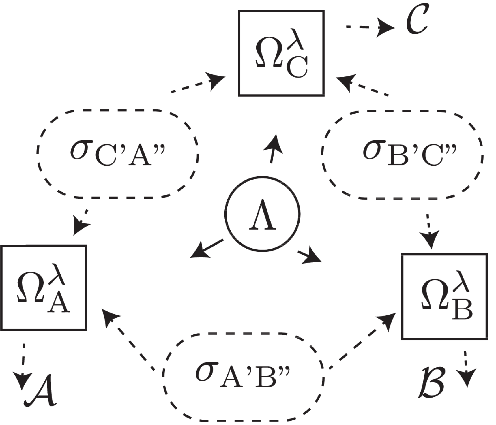
By performing local tomography on the state $\rho_{\mathcal{ABC}}$, can Alice, Bob and Charlie certify that the state produced by Eve’s network is indeed a valuable tripartite quantum state?

The family of states that they try to rule out can be defined formally. Let $\Lambda$ be a classical random variable with distribution $P_{\Lambda}(\lambda)$ sent to the three labs (for example through radio broadcast). Denoting by $\mathsf{B}(\mathcal{H})$ the set of bounded operators on the Hilbert space $\mathcal{H}$, we describe the deterministic operation at Alice’s by a family of linear maps $\left\{\Omega_{\mathcal{A}}^{\lambda}\right\}_{\lambda}$, where each $\Omega_{\mathcal{A}}^{\lambda}$ has type

and each $\Omega_{\mathcal{A}}^{\lambda}$ is completely positive and trace preserving. For completeness, the other maps correspond to $\Omega_{\mathcal{B}}^{\lambda}:\mathsf{B}(\mathcal{B}^{\prime}\otimes\mathcal{B}^{\prime\prime})\rightarrow\mathsf{B}(\mathcal{B})$ and $\Omega_{\mathcal{C}}^{\lambda}:\mathsf{B}(\mathcal{C}^{\prime}\otimes\mathcal{C}^{\prime\prime})\rightarrow\mathsf{B}(\mathcal{C})$, so that the state $\rho_{\mathcal{ABC}}$ is

where $\sigma=\sigma_{\mathcal{A^{\prime}B^{\prime\prime}}}\otimes\sigma_{\mathcal{B^{\prime}C^{\prime\prime}}}\otimes\sigma_{\mathcal{C^{\prime}A^{\prime\prime}}}$.

The valuable states, those genuinely network 3-entangled, are those that cannot be written the way described by Eq. (4). It is easy to see that the set of states of the form of Eq. (4) is closed under tensor products and LOSR transformations. That is, the set of network $2$-entangled states is a self-contained class within the resource theory of LOSR entanglement Buscemi 2012; Schmid et al. 2020a. This property has obvious implications for the monotonicity of any network $3$-entanglement measure. Think for instance of the robustness of entanglement Vidal and Tarrach 1999. We could define its network $3$-entanglement generalization as the minimum amount of network $2$-entangled noise $R(\rho_{\mathcal{A}\mathcal{B}\mathcal{C}})$ which one must add to a tripartite quantum state $\rho_{\mathcal{A}\mathcal{B}\mathcal{C}}$ to make it network $2$-entangled. Closure under LOSR implies that $R(\rho_{\mathcal{A}\mathcal{B}\mathcal{C}})$ is monotonically decreasing under LOSR operations. From our motivating discussion, though, it follows that $R(\rho_{\mathcal{A}\mathcal{B}\mathcal{C}})$ can be arbitrarily increased by means of LOCC protocols.

Note that, in the considered adversarial scenario, rather than the state $\sigma_{\mathcal{A}^{\prime}\mathcal{B}^{\prime\prime}}\otimes\sigma_{\mathcal{C}^{\prime}\mathcal{A}^{\prime\prime}}\otimes\sigma_{\mathcal{B}^{\prime}\mathcal{C}^{\prime\prime}}$, Eve could also distribute Alice, Bob and Charlie arbitrary convex combinations of states of the form $\sigma^{(i)}_{\mathcal{A}^{\prime}\mathcal{B}^{\prime\prime}}\otimes\sigma^{(i)}_{\mathcal{C}^{\prime}\mathcal{A}^{\prime\prime}}\otimes\sigma^{(i)}_{\mathcal{B}^{\prime}\mathcal{C}^{\prime\prime}}$, for some values of $i$. Since the dimensionality of the primed spaces is unbounded, though, this strategy can be simulated with the operations allowed by Eq. (4). Indeed, it suffices to distribute the tensor product of the states $\sigma^{(i)}_{\mathcal{A}^{\prime}\mathcal{B}^{\prime\prime}}\otimes\sigma^{(i)}_{\mathcal{C}^{\prime}\mathcal{A}^{\prime\prime}}\otimes\sigma^{(i)}_{\mathcal{B}^{\prime}\mathcal{C}^{\prime\prime}}$ and embed the index $i$ within the hidden variable $\Lambda$ (whose dimension is also unbounded). The index $i$ would then signal in which pair of Hilbert spaces at party $Z$’s the map $\Omega_{\mathcal{Z}}^{\lambda}$ is to be applied.

The definition of genuine network entanglement can be straightforwardly extended to the $n$-partite case.

The certification of $\rho_{\mathcal{ABC}}$ being genuinely network $3$-entangled is complicated, as the dimensions of the Hilbert spaces $\mathcal{A}^{\prime},\ldots,\,\mathcal{C}^{\prime\prime}$ are in principle unbounded. To classify the degree of a state’s network multipartiteness, we must somehow determine if the state can come about from a particular quantum causal process. The study of quantum causal processes has experienced great progress Chaves et al. 2015; Costa and Shrapnel 2016; Allen et al. 2017; Wolfe et al. 2019; Barrett et al. 2019, and many techniques have recently been developed Wolfe et al. 2019; Pozas-Kerstjens et al. 2019; Bowles et al. 2020. Herein, we adapt the inflation technique for causal inference Wolfe et al. 2019; Wolfe et al. 2019 in order derive witnesses for genuine network entanglement.

As a starter, we consider a three qudit state $\rho_{\mathcal{A}\mathcal{B}\mathcal{C}}$, and quantify its proximity to the Greenberger-Horne-Zeilinger (GHZ) state Greenberger et al. 1989 via the fidelity

If $\rho_{\mathcal{ABC}}$ is of the form of Eq. (4), then there exists a random variable $\Lambda$, quantum states $\sigma_{\mathcal{A^{\prime}B^{\prime\prime}}}$, $\sigma_{\mathcal{B^{\prime}C^{\prime\prime}}}$ and $\sigma_{\mathcal{C^{\prime}A^{\prime\prime}}}$ and families of completely positive and trace-preserving (CPTP) maps $\left\{\Omega_{\mathcal{A}}^{\lambda}\right\}_{\lambda}$, $\left\{\Omega_{\mathcal{B}}^{\lambda}\right\}_{\lambda}$ and $\left\{\Omega_{\mathcal{C}}^{\lambda}\right\}_{\lambda}$ that generate $\rho_{\mathcal{ABC}}$. To derive bounds on the maximum fidelity achievable by network $2$-entangled states, we next imagine what states one could prepare by combining multiple realizations of the above state and channel resources. As we will see, some of the reduced density matrices of the resulting many-body inflated states are fully determined by the original tripartite state $\rho_{\mathcal{A}\mathcal{B}\mathcal{C}}$. The property of $\rho_{\mathcal{A}\mathcal{B}\mathcal{C}}$ admitting a decomposition of the form of Eq. (4) will then be relaxed to that of admitting positive semidefinite inflated states satisfying said linear constraints. In the language of Wolfe et al. 2019, we will be defining a nonfanout inflation of the causal scenario depicted in Figure 1.

In this regard, consider the ring inflation scenario depicted in Figure 2. If one acts on two copies of the states $\sigma_{\mathcal{A^{\prime}B^{\prime\prime}}}$, $\sigma_{\mathcal{B^{\prime}C^{\prime\prime}}}$ and $\sigma_{\mathcal{C^{\prime}A^{\prime\prime}}}$ with the maps $\left\{\Omega_{\mathcal{A}}^{\lambda}\right\}_{\lambda}$, $\left\{\Omega_{\mathcal{B}}^{\lambda}\right\}_{\lambda}$ and $\left\{\Omega_{\mathcal{C}}^{\lambda}\right\}_{\lambda}$ in the ways indicated in the figure, one obtains the six-partite density matrices $\tau_{\mathcal{A}_{1}\mathcal{B}_{1}\mathcal{C}_{1}\mathcal{A}_{2}\mathcal{B}_{2}\mathcal{C}_{2}}$ and $\gamma_{\mathcal{A}_{3}\mathcal{B}_{3}\mathcal{C}_{3}\mathcal{A}_{4}\mathcal{B}_{4}\mathcal{C}_{4}}$. Those are essentially unknown to us, as we do not know how Eve’s devices act when they are wired differently.

Let us now provide some intuition as to why any state $\rho_{\mathcal{A}\mathcal{B}\mathcal{C}}$ admitting such extensions ${\tau,\gamma}$ cannot be arbitrarily close to the GHZ state. Suppose, indeed, that $F_{\mathsf{GHZ}_{d}}=1$, i.e., $\rho_{\mathcal{A}\mathcal{B}\mathcal{C}}=|\mathsf{GHZ}_{d}\rangle\!\langle\mathsf{GHZ}_{d}|$ and that there exist extensions ${\gamma,\tau}$ satisfying the constraints above. A measurement in the computational basis of the sites ${\mathcal{A}_{3},\mathcal{B}_{3},\mathcal{C}_{3}}$ of $\gamma$ will generate the random variables ${a_{3},b_{3},c_{3}}$. Since $\gamma_{(\mathcal{A}_{3}\mathcal{B}_{3})}=\rho_{(\mathcal{A}\mathcal{B})}=\frac{1}{d}\sum_{i=1}^{d}|i,i\rangle\!\langle i,i|$, it must be the case that ${a_{3},b_{3}}$ are perfectly correlated. The same considerations hold for $b_{3}$ and $c_{3}$. Since ${a_{3},b_{3}}$ and ${b_{3},c_{3}}$ are pair-wise perfectly correlated, so are ${a_{3},c_{3}}$. Now, from the condition $\gamma_{\left(\mathcal{C}_{3}\mathcal{A}_{4}\mathcal{C}_{4}\mathcal{A}_{3}\right)}=\tau_{\left(\mathcal{C}_{2}\mathcal{A}_{2}\mathcal{C}_{1}\mathcal{A}_{1}\right)}$, we have that the distribution of $c_{3}$ and $a_{3}$ must be the same as that of $c_{2}$ and $a_{1}$. Hence, $c_{2}$ and $a_{1}$ must be perfectly correlated. However, $\tau_{(\mathcal{A}_{1}\mathcal{B}_{1}\mathcal{C}_{1})}$ is a pure state, since $\tau_{(\mathcal{A}_{1}\mathcal{B}_{1}\mathcal{C}_{1})}=\rho_{\mathcal{A}\mathcal{B}\mathcal{C}}=|\mathsf{GHZ}_{d}\rangle\!\langle\mathsf{GHZ}_{d}|$, and hence it must be in a product state with respect to any other system, such as $\mathcal{C}_{2}$. It follows that a measurement in the computational basis of the sites $\mathcal{A}_{1}$ and $\mathcal{C}_{2}$ will produce two uncorrelated random variables ${a_{1},c_{2}}$. We thus reach a contradiction.

For $d{=}2$, Eq. (9) establishes that any tripartite state with $F_{\mathsf{GHZ}_{2}}>\frac{4}{33}\left(6+\sqrt{3}\right)\approx 0.9372$ is genuinely network $3$-entangled. As it turns out, this inequality is not tight: it can be improved to $F_{\mathsf{GHZ}_{2}}>\frac{1+\sqrt{3}}{4}\approx 0.6803$ by means of semidefinite programming applied to the ring inflation.

The variables in the corresponding program are trace-one positive semidefinite matrices $\tau_{\mathcal{A}_{1}\mathcal{B}_{1}\mathcal{C}_{1}\mathcal{A}_{2}\mathcal{B}_{2}\mathcal{C}_{2}}$ and $\gamma_{\mathcal{A}_{3}\mathcal{B}_{3}\mathcal{C}_{3}\mathcal{A}_{4}\mathcal{B}_{4}\mathcal{C}_{4}}$ of size $64\times 64$, subject to linear constraints of the form of Eqs. (6) and (7), as well as to the permutational symmetry $1\leftrightarrow 2$, $3\leftrightarrow 4$. For all states $\mu_{\mathcal{X}\mathcal{Y}}$ separable across a $\mathcal{X}/\mathcal{Y}$ partition, we add a Positivity under Partial Transposition (PPT) constraint ${\left(\mu_{\mathcal{X}\mathcal{Y}}\right)^{{}_{\top_{\mathcal{Y}}}}\!\!\!\underaccent{\mathsf{PSD}}{\succeq}0}$ Peres 1996. This applies to $\tau$ across the $\mathcal{A}_{1}\mathcal{B}_{1}\mathcal{C}_{1}/\mathcal{A}_{2}\mathcal{B}_{2}\mathcal{C}_{2}$ partition, and to reduced states of $\gamma$ for the partitions $\mathcal{A}_{3}\mathcal{B}_{3}\mathcal{C}_{3}/\mathcal{B}_{4}$, $\mathcal{B}_{3}\mathcal{C}_{3}\mathcal{A}_{4}/\mathcal{C}_{4}$, $\mathcal{C}_{3}\mathcal{A}_{4}\mathcal{B}_{4}/\mathcal{A}_{3}$.

The bound $F_{\mathsf{GHZ}_{2}}>\frac{1+\sqrt{3}}{4}$ is obtained by maximizing $\left\langle\mathsf{GHZ}_{2}\middle|\rho_{\mathcal{ABC}}\middle|\mathsf{GHZ}_{2}\right\rangle$ subject to the constraints above—a typical instance of a semidefinite program—using the optimization toolbox CVX Grant and Boyd 2020 and the solver Mosek MOSEK ApS 2019.

We also employed the semidefinite optimization procedure using as reference the W state Dür et al. 2000, ${|\mathsf{W}\rangle\equiv\,\displaystyle\frac{|001\rangle+|010\rangle+|100\rangle}{\sqrt{3}}}$, concluding that any $3$-qubit state $\rho_{\mathcal{ABC}}$ with $\langle\mathsf{W}|\rho_{\mathcal{ABC}}|\mathsf{W}\rangle>0.7602$ is genuinely network $3$-entangled.

Armed with these witnesses, we find that several past experiments in quantum optics can be interpreted as demonstrations of genuine network tripartite entanglement Erdösi et al. 2013; Hübel et al. 2010; Resch et al. 2005; Walther et al. 2005. Indeed, in all those experiments, the fidelity of the prepared states with respect to GHZ or W states is greater than the bounds derived above for network-bipartite states. The prepared states are thus certified to contain genuine network tripartite entanglement.

In many experimental setups, due to low detector efficiencies, the carriers transmitting the quantum information are often unobserved. The standard prescription in such a predicament consists in discarding the experimental data gathered when not all detectors click. Coming back to our adversarial setup, this postselection of measurement results opens a loophole that Eve can in principle exploit to fool Alice, Bob, and Charlie. It is possible to contemplate this contingency in the calculations above, and thus bound the detection efficiency needed for certifying genuine network entanglement under post-selection.

Let $p$ indicate the fraction of experimental data preserved by postselection, i.e., the probability that all three detectors click. If $\rho^{p}_{\mathcal{ABC}}$ is the state reconstructed after postselection, then all that can be said about the true tripartite quantum state $\rho_{\mathcal{ABC}}$ before the postselection took place is that

As before, linear optimizations over the set of postselected states $\rho^{p}_{\mathcal{ABC}}$ can be conducted via semidefinite programming. In such instances one continues to relate the inflated states $\tau$ and $\gamma$ to the true (albeit unknown) tripartite state $\rho_{\mathcal{ABC}}$, and Eq. (10) is merely added as an extra constraint. We find critical postselection probabilities beyond which one can still certify genuine network tripartite entanglement via GHZ fidelity ($p_{c}\approx 0.685$) or W fidelity ($p_{c}\approx 0.765$).

In this paper we have argued that the standard definition of genuine multipartite entanglement is not appropriate to assess the quantum control over an ever-growing number of quantum systems. We proposed an alternative definition, genuine network multipartite entanglement, that captures the potential of a source to distribute entanglement over a number of spatially separated parties. We provided analytic and numerical tools to detect genuine network tripartite entanglement, and also indicated how the definition can be adapted to situations where there may be local postselections on each party’s lab. Furthermore, the construction can be adapted to detect genuine network $n$-partite entanglement for any $n$.

While quite general, our numerical methods to detect genuine network entanglement demand considerable memory resources to the point that we were not able to derive new entanglement witnesses for tripartite qutrit states in a normal computer. In addition, there exist significant gaps between the bounds we derived on GHZ and W state fidelities via SDP relaxations and the lower bounds obtained using standard variational techniques Werner and Wolf 2001; Pál and Vértesi 2010. Using such algorithms, we were not able to give lower bounds to the GHZ and W fidelities larger than $0.5170$ and $2/3$, respectively. A topic for future research is thus to develop better techniques for the characterization of genuine network multipartite entanglement.

After completing this manuscript, we became aware of the work of Kraft et al. 2020; Luo 2020, whose authors consider a scenario very similar to that depicted in Figure 1. Crucially, they restrict the maps $\Omega^{\lambda}_{\mathcal{A},\mathcal{B},\mathcal{C}}$ to be unitary transformations, acting on convex combinations of bipartite states. The restriction to unitary maps not only allows upper-bounding the dimensionality of the source states $\sigma_{\mathcal{A}^{\prime}\mathcal{B}^{\prime\prime}},\sigma_{\mathcal{C}^{\prime}\mathcal{A}^{\prime\prime}},\sigma_{\mathcal{B}^{\prime}\mathcal{C}^{\prime\prime}}$, but it also severely constrains the resulting set of states $\Delta_{C}$: as shown in Kraft et al. 2020, tripartite qubit states in $\Delta_{C}$ cannot be genuinely tripartite entangled. This contrasts with the GHZ fidelity greater than $1/2$ reported above, achievable by states of the form of Eq. (4).

We thank Antonio Acín, Jean-Daniel Bancal, T.C. Fraser, Yeong-Cherng Liang, David Schmid, and Robert W. Spekkens for useful discussions. M.N. was supported by the Austrian Science fund (FWF) stand-alone project P 30947. The work of A.P.-K. was supported by Fundació Obra Social “la Caixa” (LCF/BQ/ES15/10360001), the ERC (CoG QITBOX and the European Union’s Horizon 2020 research and innovation programme - grant agreement No 648913), the Spanish MINECO (FIS2016-80773-P and Severo Ochoa SEV-2015-0522), Fundació Cellex, and Generalitat de Catalunya (SGR 1381 and CERCA Programme). This research was supported by Perimeter Institute for Theoretical Physics. Research at Perimeter Institute is supported in part by the Government of Canada through the Department of Innovation, Science and Economic Development Canada and by the Province of Ontario through the Ministry of Economic Development, Job Creation and Trade. This publication was made possible through the support of a grant from the John Templeton Foundation. The opinions expressed in this publication are those of the authors and do not necessarily reflect the views of the John Templeton Foundation.

References

- Bennett et al. (1993) C. H. Bennett, G. Brassard, C. Crépeau, R. Jozsa, A. Peres, and W. K. Wootters, Teleporting an unknown quantum state via dual classical and Einstein-Podolsky-Rosen channels, Phys. Rev. Lett. 70, 1895 (1993).
- Bennett and Wiesner (1992) C. H. Bennett and S. J. Wiesner, Communication via one- and two-particle operators on Einstein-Podolsky-Rosen states, Phys. Rev. Lett. 69, 2881 (1992).
- Scarani et al. (2009) V. Scarani, H. Bechmann-Pasquinucci, N. J. Cerf, M. Dušek, N. Lütkenhaus, and M. Peev, The security of practical quantum key distribution, Rev. Mod. Phys. 81, 1301 (2009).
- Bell (1964) J. S. Bell, On the Einstein-Podolsky-Rosen paradox, Physics 1, 195 (1964).
- Brunner et al. (2014) N. Brunner, D. Cavalcanti, S. Pironio, V. Scarani, and S. Wehner, Bell nonlocality, Rev. Mod. Phys. 86, 419 (2014).
- Lu et al. (2007) C.-Y. Lu, X.-Q. Zhou, O. Gühne, W.-B. Gao, J. Zhang, Z.-S. Yuan, A. Goebel, T. Yang, and J.-W. Pan, Experimental entanglement of six photons in graph states, Nat. Phys. 3, 91 (2007).
- Yao et al. (2012) X.-C. Yao, T.-X. Wang, P. Xu, H. Lu, G.-S. Pan, X.-H. Bao, C.-Z. Peng, C.-Y. Lu, Y.-A. Chen, and J.-W. Pan, Observation of eight-photon entanglement, Nat. Phot. 6, 225 (2012).
- Wang et al. (2016) X.-L. Wang, L.-K. Chen, W. Li, H.-L. Huang, C. Liu, C. Chen, Y.-H. Luo, Z.-E. Su, D. Wu, Z.-D. Li, H. Lu, Y. Hu, X. Jiang, C.-Z. Peng, L. Li, N.-L. Liu, Y.-A. Chen, C.-Y. Lu, and J.-W. Pan, Experimental ten-photon entanglement, Phys. Rev. Lett. 117, 210502 (2016).
- Gross et al. (2010) C. Gross, T. Zibold, E. Nicklas, J. Estève, and M. K. Oberthaler, Nonlinear atom interferometer surpasses classical precision limit, Nature 464, 1165 (2010).
- Seevinck and Uffink (2001) M. Seevinck and J. Uffink, Sufficient conditions for three-particle entanglement and their tests in recent experiments, Phys. Rev. A 65, 012107 (2001).
- Gühne et al. (2005) O. Gühne, G. Tóth, and H. J. Briegel, Multipartite entanglement in spin chains, New J. Phys. 7, 229 (2005).
- Gühne and Tóth (2006) O. Gühne and G. Tóth, Energy and multipartite entanglement in multidimensional and frustrated spin models, Phys. Rev. A 73, 052319 (2006).
- McConnell et al. (2015) R. McConnell, H. Zhang, J. Hu, S. Cuk, and V. Vuletic, Entanglement with negative Wigner function of almost 3000 atoms heralded by one photon, Nature 519, 439 (2015).
- Allen et al. (2017) J.-M. A. Allen, J. Barrett, D. C. Horsman, C. M. Lee, and R. W. Spekkens, Quantum Common Causes and Quantum Causal Models, Phys. Rev. X 7, 031021 (2017).
- Buscemi (2012) F. Buscemi, All Entangled Quantum States Are Nonlocal, Phys. Rev. Lett. 108, 200401 (2012).
- Schmid et al. (2020a) D. Schmid, D. Rosset, and F. Buscemi, The type-independent resource theory of local operations and shared randomness, Quantum 4, 262 (2020a).
- Wolfe et al. (2020) E. Wolfe, D. Schmid, A. B. Sainz, R. Kunjwal, and R. W. Spekkens, Quantifying Bell: the resource theory of nonclassicality of common-cause boxes, Quantum 4, 280 (2020).
- Schmid et al. (2020b) D. Schmid, T. C. Fraser, R. Kunjwal, A. B. Sainz, E. Wolfe, and R. W. Spekkens, Why standard entanglement theory is inappropriate for the study of Bell scenarios (2020b), arXiv:2004.09194 .
- Vidal and Tarrach (1999) G. Vidal and R. Tarrach, Robustness of entanglement, Phys. Rev. A 59, 141 (1999).
- Chaves et al. (2015) R. Chaves, C. Majenz, and D. Gross, Information–theoretic implications of quantum causal structures, Nat. Comm. 6 (2015).
- Costa and Shrapnel (2016) F. Costa and S. Shrapnel, Quantum causal modelling, New J. Phys. 18, 063032 (2016).
- Wolfe et al. (2019) E. Wolfe, A. Pozas-Kerstjens, M. Grinberg, D. Rosset, A. Acín, and M. Navascues, Quantum Inflation: A General Approach to Quantum Causal Compatibility (2019), arXiv:1909.10519 .
- Barrett et al. (2019) J. Barrett, R. Lorenz, and O. Oreshkov, Quantum Causal Models (2019), arXiv:1906.10726 .
- Pozas-Kerstjens et al. (2019) A. Pozas-Kerstjens, R. Rabelo, L. Rudnicki, R. Chaves, D. Cavalcanti, M. Navascués, and A. Acín, Bounding the Sets of Classical and Quantum Correlations in Networks, Phys. Rev. Lett. 123 (2019).
- Bowles et al. (2020) J. Bowles, F. Baccari, and A. Salavrakos, Bounding sets of sequential quantum correlations and device-independent randomness certification, Quantum 4, 344 (2020).
- Wolfe et al. (2019) E. Wolfe, R. W. Spekkens, and T. Fritz, The Inflation Technique for Causal Inference with Latent Variables, J. Causal Inference 7 (2019).
- Greenberger et al. (1989) D. M. Greenberger, M. A. Horne, and A. Zeilinger, Going beyond Bell’s theorem, in Bell’s Theorem, Quantum Theory and Conceptions of the Universe, edited by M. Kafatos (Springer Netherlands, Dordrecht, 1989) pp. 69–72.
- Peres (1996) A. Peres, Separability Criterion for Density Matrices, Phys. Rev. Lett. 77, 1413 (1996).
- Grant and Boyd (2020) M. Grant and S. Boyd, CVX: Matlab Software for Disciplined Convex Programming, version 2.2, http://cvxr.com/cvx (2020).
- MOSEK ApS (2019) MOSEK ApS, The MOSEK optimization toolbox for MATLAB manual, https://docs.mosek.com (2019).
- Dür et al. (2000) W. Dür, G. Vidal, and J. I. Cirac, Three qubits can be entangled in two inequivalent ways, Phys. Rev. A 62, 062314 (2000).
- Erdösi et al. (2013) D. Erdösi, M. Huber, B. C. Hiesmayr, and Y. Hasegawa, Proving the generation of genuine multipartite entanglement in a single-neutron interferometer experiment, New J. Phys. 15, 023033 (2013).
- Hübel et al. (2010) H. Hübel, D. R. Hamel, A. Fedrizzi, S. Ramelow, K. J. Resch, and T. Jennewein, Direct generation of photon triplets using cascaded photon-pair sources, Nature 466, 601 (2010).
- Resch et al. (2005) K. J. Resch, P. Walther, and A. Zeilinger, Full Characterization of a Three-Photon Greenberger-Horne-Zeilinger State Using Quantum State Tomography, Phys. Rev. Lett. 94, 070402 (2005).
- Walther et al. (2005) P. Walther, K. J. Resch, and A. Zeilinger, Local Conversion of Greenberger-Horne-Zeilinger States to Approximate States, Phys. Rev. Lett. 94, 240501 (2005).
- Werner and Wolf (2001) R. F. Werner and M. M. Wolf, All multipartite Bell correlation inequalities for two dichotomic observables per site, Phys. Rev. A 64, 1 (2001).
- Pál and Vértesi (2010) K. F. Pál and T. Vértesi, Maximal violation of a bipartite three-setting, two-outcome Bell inequality using infinite-dimensional quantum systems, Phys. Rev. A 82, 022116 (2010).
- Kraft et al. (2020) T. Kraft, S. Designolle, C. Ritz, N. Brunner, O. Gühne, and M. Huber, Quantum entanglement in the triangle network (2020), arXiv:2002.03970 .
- Luo (2020) M.-X. Luo, New genuine multipartite entanglement (2020), arXiv:2003.07153 .
Appendix A Appendix A: analytic witnesses for
genuine network tripartite entanglement
The goal of this appendix is to prove the following result:
Theorem 1.
Let be a tripartite quantum state, and let be the outcomes which result when we locally probe subsystems . If is not genuinely network -entangled, then it must satisfy the relations: