Defects in active nematics – algorithms for identification and tracking

The model is known from liquid crystal theory as an extension of the Beris-Edwards model [14], which is here supplemented with an additional active stress term and reads [15]

with fluid velocity $\mathbf{V}$, pressure $P$, Landau-de Gennes Q-tensor $\boldsymbol{Q}$, order parameter $S$, flow alignment parameter $\lambda$, rotational viscosity $\gamma$, Reynolds number $\mathrm{Re}$, additional stress $\boldsymbol{\sigma}=\boldsymbol{\sigma}^{\textup{A}}+\boldsymbol{\sigma}^{\textup{B}}$ with active stress $\boldsymbol{\sigma}^{\textup{A}}=\alpha\boldsymbol{Q}$ and an elastic stress $\boldsymbol{\sigma}^{\textup{B}}=\boldsymbol{Q}\boldsymbol{H}-\boldsymbol{H}\boldsymbol{Q}-\lambda\boldsymbol{H}$, the molecular field $\boldsymbol{H}=L\boldsymbol{\Delta}\boldsymbol{Q}-a\boldsymbol{Q}+b(\boldsymbol{Q}^{2}-\frac{1}{3}\operatorname{trace}(\boldsymbol{Q}^{2})\mathbf{I})-c\operatorname{trace}(\boldsymbol{Q}^{2})\boldsymbol{Q}$, deformation tensor $\boldsymbol{D}=\frac{1}{2}(\nabla\mathbf{V}+(\nabla\mathbf{V})^{T})$ and vorticity tensor $\boldsymbol{\Omega}=\frac{1}{2}(\nabla\mathbf{V}-(\nabla\mathbf{V})^{T})$, with $\alpha,L,a,b,c\in\mathbb{R}$. The model considers only a one-constant approximation of the Landau-de-Gennes energy (see [16] for more general expressions) and assumes only the simplest possible form of an active stress. We further have neglected the Ericksen stress. Supplemented with initial and boundary conditions the system without activity, $\alpha=0$, has been analysed and numerically solved in [17]. We here adapt this numerical approach and solve the system in a square domain in 2D with periodic boundary conditions. Fig. 1 shows a time instant of a simulation.

For simplicity we consider a modeling approach without hydrodynamics. For hydrodynamic interactions we refer to [19]. The model and numerical approaches to solve it have been introduced in [20, 21]. Modified versions for active and passive systems can be found in [22, 23, 24, 25, 26] and [27], respectively. We model each cell by a phase field active polar gel model [28] and consider a short-range interaction potential between them. The evolution equations read

for $i=1,\ldots,n$ phase field variables $\phi_{i}$ and polarization fields $\mathbf{P}_{i}$. The parameters $Ca$, $Pa$ and $In$ act as weightings between different energy contributions, a classical Ginzburg-Landau function with double-well potential $W(\phi)=\frac{1}{4}(\phi^{2}-1)^{2}$ and interface thickness $\epsilon$, a polar liquid crystal energy of Frank-Oseen type, with $c$ and $\beta$ parameters controlling the deformation of the polarization fields $\mathbf{P}_{i}$ and the anchoring on the cell interface, respectively, and the interaction term, which considers $B(\phi_{i})=\frac{3}{\epsilon\sqrt{2}}W(\phi_{i})\approx\delta_{\Gamma_{i}}$ as an approximation of the surface delta function for the cell boundary $\Gamma_{i}=\{\mathbf{x}\in\Omega\;|\;\phi_{i}(\mathbf{x})=0\}$ and an approximation of an interaction potential $w(d_{j})=\exp(-d_{j}^{2}/\epsilon^{2})$ with signed distance function $d_{j}(\phi_{j})=-\frac{\epsilon}{\sqrt{2}}\ln((1+\phi_{j}(\mathbf{x}))/(1-\phi_{j}(\mathbf{x})))$ with respect to the zero-line (cell boundary $\Gamma_{j}$) of $\phi_{j}$. Activity is introduced in the evolution equations by a self-propulsion term, with velocity value $v_{0}$. For a detailed description of the numerical approach we refer to [29].

In order to analyse emerging nematic properties we define for each phase field variable $\phi_{i}$ a Q-tensor by

and obtain a continuous Q-tensor field $\mathbf{Q}$ by interpolating between these tensors in the center of mass in each cell. Fig. 2 shows a time instant of a simulation with $n=100$ cells.

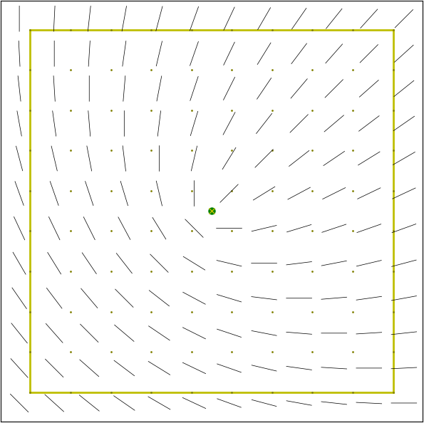
Topological defects are characterized as degenerated points of $\mathbf{Q}$ for which $Q_{11}=Q_{12}=0$. For a nematic liquid crystal in 2D two types of topological defects predominate: comet-like ($+\frac{1}{2}$) and trefoil-like ($-\frac{1}{2}$). The number associated with the topological defects, the winding number or topological charge, is the change in the orientation around the singular points along a full $2\pi$ rotation, divided by $2\pi$: for $+\frac{1}{2}$ and $-\frac{1}{2}$ defects the orientation field rotates by $+\pi$ and $-\pi$, respectively, see Fig. 3.

We consider two approaches to identify the topological charge of the defects. The first is physics based and considers the sign of $\delta=\frac{\partial Q_{11}}{\partial x}\frac{\partial Q_{12}}{\partial y}-\frac{\partial Q_{11}}{\partial y}\frac{\partial Q_{12}}{\partial x}$ to distinguish between $+\frac{1}{2}$ and $-\frac{1}{2}$ defects. The second treats the task as an image processing problem and uses an artificial neural network (ANN) to identify the defect type. The neural network consists of an input layer with 100 nodes, two hidden layers with 1000 and 200 nodes, respectively, and an output layer with two nodes, one for $+\frac{1}{2}$ and $-\frac{1}{2}$ defects. For every degenerated point of $\mathbf{Q}$, a $10\!\times\!10$ grid, called kernel, with the defect located in the center, is computed by interpolation. This kernel data serves as input, see Fig. 4. The training data is constructed analytically by specifying boundary conditions for vector fields. We consider 5000 simulated defects for each topological charge. To generate a decent variability, the defect is affected by surrounding defects and noise. Each data is trained within five epochs with a learning rate of $0.05$. Tests on ideal, single affected and multiple combined defect data have been performed leading to identification rates of $96.98\,\%$. More comprehensive network constructions and more extensive training processes would lead to higher precision. Applied to the simulation data, the classification with the ANN yields an identification rate of $99.31\,\%$.

With known defect positions and type in each time frame we have to connect them from frame to frame. Dozens of software tools have been developed for this task in the context of particle tracking [30]. For a comparison of these methods we refer to [31]. We here use an approach described in [32]. It involves finding a set of associations between the defect locations in subsequent frames such that a cost functional is minimized. It is based on a particle matching algorithm using a graph theory technique. It allows to consider different defect types and defect appearance and disappearance and is available as a plugin for ImageJ and Fiji (www.imagej.net) [33].

Using the described tools for defect identification and tracking, we can statistically examine the velocity distribution of topological defects. We compute these data for both models and compare them with experimental data. However, due to a lack of available data for defects in epithelia tissue, we here compare both with data for MT bundles [34]. Similar comparisons, with a higher order Landau-de Gennes model have been performed in [35]. As both of our models are written in dimensionless units we first rescale our data based on the reported average velocity of $6.6\mu ms^{-1}$ in [35]. Figure 5 shows the comparison for both models for $+\frac{1}{2}$ and $-\frac{1}{2}$ defects. We observe an excellent agreement of the experimental data with the active nematodynamics model of section 2.1. The results also show a significant difference in the velocity distribution between $+\frac{1}{2}$ and $-\frac{1}{2}$ defects. $+\frac{1}{2}$ defects are significantly faster, which again is in agreement with experimental data and theoretical predictions [5]. This difference is still present in the multi-phase field model of section 2.2, but much less pronounced. The velocity distributions for $+\frac{1}{2}$ and $-\frac{1}{2}$ defects are almost equal to each other in this model.

We can also analyse the direction of defect movement. In the active nematodynamics model $+\frac{1}{2}$ defects move in the direction of the ’tail’ of the defect, indicating contractile systems. The direction of movement can be tuned by the sign of $\alpha$ in the active stress. For the multi-phase field model, this is less obvious, as the defects are a secondary effect and not directly related to movement. However, also in these systems contractile behavior is most common, which again is in agreement with experimental measurements [9].

Another example which shows qualitative agreement with experimental data is achieved by considering the multi-phase field model described in Section 2.2 with 100 cells in a square confinement. Within a certain activity range this leads to oscillations in the cell movements. These oscillations are in qualitative agreement with results on microscopy images of human keratinocytes (HaCaT cells) in similar confinements, see [36]. Figure 6 visualizes the trajectories of the centers of mass for some cells and compares them with the experimental data.

The same methodology to identify, classify and track defects is applicable to experimental data. Instead of the numerical solution it just requires an image processing step to map microscopy images to Q-tensor fields. For epithelia tissue this requires a classical segmentation problem to identify each cell, which than can be represented by a phase field variable, which can be processed as in Sec. 2. For filamentous particles, e.g. MT bundles the directional field has to be estimated. This can be done be computing a gradient vector on the gray-scale image for each pixel and appropriately averaging by first doubling the angle and squaring the length to account for the head-tail symmetry. In [37] it is shown that this approach is equivalent to a principal component analysis and robustly leads to directional fields $\mathbf{n}$. The Q-tensor field can than be computed by $\mathbf{Q}=S(\mathbf{n}\otimes\mathbf{n}-\frac{1}{2}\mathbf{I})$ with $S$ the scalar order parameter, encoding the degree of alignment with the average direction and $\mathbf{I}$ the identity matrix. Detailed comparisons on defects between experimental and simulation data will be done elsewhere based on the proposed algorithms.

References

- [1] M.C. Marchetti, J.F. Joanny, S. Ramaswamy, T. B. Liverpool, J. Prost, M. Rao, and R.A. Simha. Hydrodynamics of soft active matter. Rev. Mod. Phys., 85:1143–1189, 2013.
- [2] A.M. Menzel. Tuned, driven, and active soft matter. Phys. Rep., 554:1–45, 2015.
- [3] J. Prost, F. Jülicher, and J.-F. Joanny. Active gel physics. Nature Phys., 11:111–117, 2015.
- [4] F. Jülicher, S.W. Grill, and G. Salbreux. Hydrodynamic theory of active matter. Rep. Prog. Phys., 81:076601, 2018.
- [5] A. Doostmohammadi, J. Ignes-Mullol, J.M. Yeomans, and F. Sagues. Active nematics. Nature Comm., 9:3246, 2018.
- [6] L. Giomi, M.J. Bowick, P. Mishra, R. Sknepnek, and M.C. Marchetti. Defect dynamics in active nematics. Phil. Trans. Roy. Soc. A, 372:20130365, 2014.
- [7] T. Sanchez, D.T.N. Chen, S.J. DeCamp, N. Heymann, and Z. Dogic. Spontaneous motion in hierarchically assembled active matter. Nature, 491:431–434, 2012.
- [8] C. Blanch-Mercader, V Yashunsky, S. Garcia, G. Duclos, L. Giomi, and P. Silberzan. Turbulent dynamics of epithelial cell cultures. Phys. Rev. Lett., 120:208101, 2018.
- [9] T.B. Saw, A. Doostmohammadi, V. Nier, L. Kocgozlu, S. Thampi, Y. Toyama, P. Marcq, C.T. Lim, J.M. Yeomans, and B. Ladoux. Topological defects in epithelia govern cell death and extrusion. Nature, 544:212–216, 2017.
- [10] G. Duclos, C. Erlenkamper, J.-F. Joanny, and P. Silberzan. Topological defects in confined populations of spindle-shaped cells. Nature Phys., 13:58–62, 2017.
- [11] K. Kawaguchi, R. Kageyama, and M. Sano. Topological defects control collective dynamics in neural progenitor cell cultures. Nature, 545:327–331, 2017.
- [12] S. Vey and A. Voigt. AMDiS: adaptive multidimensional simulations. Comput. Vis. Sci., 10:57–67, 2007.
- [13] T. Witkowski, S. Ling, S. Praetorius, and A. Voigt. Software concepts and numerical algorithms for a scalable adaptive parallel finite element method. Adv. Computat. Math., 41:1145–1177, 2015.
- [14] E.V. Beris and B.-J. Edwards. Thermodynamics of flowing systems with internal microstructure. Oxford University Press, 1994.
- [15] L. Giomi. Geometry and topology of turbulence in active nematics. Phys. Rev. X, 5:031003, 2015.
- [16] J.M. Ball and A. Majumdar. Nematic liquid crystals: From Maier-Saupe to a continuum theory. Molec. Crys. Liq. Cryst., 525:1–11, 2010.
- [17] H. Abels, G. Dolzmann, and Y. Liu. Well-posdness of a fully coupled Navier-Stokes/Q-tensor system with inhomogeneous boundary data. SIAM J. Math. Anal., 46:3050–3077, 2014.
- [18] D.J.G. Pearce, P.W. Ellis, A. Fernandez-Nieves, and L. Giomi. Geometrical control of active turbulence in curved topographies. Phys. Rev. Lett., 122:168002, 2019.
- [19] W. Marth and A. Voigt. Collective migration under hydrodynamic interactions: a computational approach. Interf. Focus, 6(5):20160037, 2016.
- [20] W. Marth, S. Praetorius, and A. Voigt. A mechanism for cell motility by active polar gels. J. Roy. Soc. Interf., 12:20150161, 2015.
- [21] D. Wenzel, S. Praetorius, and A. Voigt. Topological and geometrical quantities in active cellular structures. J. Chem. Phys., 150:164108, 2019.
- [22] F. Ziebert, S. Swaminathan, and I.S. Aranson. Model for self-polarization and motility of keratocyte fragments. J. R. Soc. Interface, 9:1084–1092, 2012.
- [23] B.A. Camley, Y. Zhang, B. Zhao, Y.and Li, E. Ben-Jacob, H. Levine, and W.-J. Rappel. Polarity mechanisms such as contact inhibition of locomotion regulate persistent rotational motion of mammalian cells on micropatterns. Proc. Nat. Acad. Sci. (USA), 111:14770–14775, 2014.
- [24] J. Loeber, F. Ziebert, and I.S. Aranson. Collisions of deformable cells lead to collective migration. Sci. Rep., 5:9172, 2015.
- [25] B.A. Camley and W.-J. Rappel. Physical models of collective cell motility: from cell to tissue. J. Phys. D - Appl. Phys., 50:113002, 2017.
- [26] R. Mueller, J.M. Yeomans, and A. Doostmohammadi. Emergence of active nematic behavior in monolayers of isotropic cells. Phys. Rev. Lett., 122:048004, 2019.
- [27] M. Nonomura. Study on multicellular systems using a phase field model. PLoS ONE, 7:e33501, 2012.
- [28] K. Kruse, J.F. Joanny, F. Jülicher, J. Prost, and K. Sekimoto. Asters, vortices, and rotating spirals in active gels of polar filaments. Phys. Rev. Lett., 92:078101, 2004.
- [29] S. Praetorius and A. Voigt. Collective cell behavior - a cell-based parallelization approach for a phase field active polar gel model. In K. Binder, M. Müller, and A. Trautmann, editors, NIC Symposium 2018, pages 369–376, 2018.
- [30] E. Meijering, O. Dzyubachyk, and I. Smal. Methods for cell and particle tracking. In Conn, P.M., editor, Imaging and spectroscopic analysis of living cells: Optical and specrroscopic techniques, volume 504 of Methods in Enzymology, pages 183–200. Academic Press, 2012.
- [31] N. Chenouard and et al. Objective comparison of particle tracking methods. Nature Meth., 11:281–290, 2014.
- [32] I.F. Sbalzarini and P. Koumoutsakos. Feature point tracking and trajectory analysis for video imaging in cell biology. J. Struc. Bio., 151:182–195, 2005.
- [33] J. Schindelin and et al. Fiji: an open-source platform for biological-image analysis. Nature Meth., 9:676–682, 2012.
- [34] S.J. DeCamp, G.S. Redner, A. Baskaran, M.F. Hagan, and Z. Dogic. Orientational order of motile defects in active nematics. Nature Materials, 14(11):1110–1115, 2015.
- [35] A.U. Oza and J. Dunkel. Antipolar ordering of topological defects in active liquid crystals. New Journal of Physics, 18(9):093006, 2016.
- [36] G. Peyret, R. Mueller, J. d’Alessandro, S. Begnaud, P. Marcq, R.-M. Mege, J.M. Yeomans, A. Doostmohammadi, and B. Ladoux. Sustained oscillations of epithelial cell sheets. Biophys. J., 117:464–478, 2019.
- [37] A.M. Bazan and S.H. Gerez. Systematic methods for the computation of the directional fields and singular points of fingerprints. IEEE Trans. Patt. Anal. Mach. Intell., 24:905–919, 2002.