Gapped non-liquid state (also known as fracton state) is a very special gapped quantum state of matter that is characterized by a microscopic cellular structure. Such microscopic cellular structure has a macroscopic effect at arbitrary long distances and cannot be removed by renormalization group flow, which makes gapped non-liquid state beyond the description of topological quantum field theory with a finite number of fields. Using Abelian and non-Abelian topological orders in 2-dimensional (2d) space and the different ways to glue them together via their gapped boundaries, we propose a systematic way to construct 3d gapped states (and in other dimensions). The resulting states are called cellular topological states, which include gapped non-liquid states, as well as gapped liquid states in some special cases. Some new fracton states with fractal excitations are constructed even using 2d topological order. More general cellular topological states can be constructed by connecting 2d domain walls between different 3d topological orders. The constructed cellular topological states can be viewed as fixed-point states for a reverse renormalization of gapped non-liquid states.
A systematic construction of gapped non-liquid states
I Introduction
Different phases of matter are not only characterized by their symmetry breaking patterns.Landau 1937a; Landau 1937b Even systems without any symmetry can have many distinct gapped zero-temperature phases, characterized by different patterns of long range quantum entanglementChen et al. 2010. Those gapped phases include gapped liquid phasesZeng and Wen 2015; Swingle and McGreevy 2016 [which incluse phases with topological ordersWen 1989; Wen 1990; Keski-Vakkuri and Wen 1993, symmetry enriched topological (SET) ordersWen 2002; Essin and Hermele 2013; Hung and Wan 2013; Xu 2013; Mesaros and Ran 2013; Chen et al. 2015; Chang et al. 2015; Cheng et al. 2017; Heinrich et al. 2016 and symmetry protected trivial (SPT) ordersGu and Wen 2009; Chen et al. 2011a; Chen et al. 2013], as well as gapped non-liquid phasesChamon 2005; Haah 2011, such as foliated phasesZeng and Wen 2015; Shirley et al. 2018; Shirley et al. 2019 (i.e. type-I fracton phasesVijay et al. 2016).
So far, we have a nearly complete understanding gapped liquid phases for boson and fermion systems with and without symmetry. In 1+1D, all gapped phases are liquid phases. They are classified by Chen et al. 2011b; Schuch et al. 2011, where is the symmetry group of the Hamiltonian, the symmetry group of the ground state , and is a group 2-cocycle for the unbroken symmetry group .
In 2+1D, we believe that all gapped phases are liquid phases. They are classified (up to invertible topological orders and for a finite unitary on-site symmetry ) by for bosonic systems and by for fermionic systemsBarkeshli et al. 2014; Lan et al. 2017; Lan et al. 2016. Here is symmetric fusion category formed by representations of , and is symmetric fusion category formed by -graded (i.e. fermion graded) representations of . Also is a braided fusion category and is a minimal modular extensionLan et al. 2017; Lan et al. 2016.
In 3+1D, some gapped phases are liquid phases while others are non-liquid phases. The 3+1D gapped liquid phases without symmetry for bosonic systems (i.e. 3+1D bosonic topological orders) are classified by Dijkgraak-Witten theories if the point-like excitations are all bosons, by twisted 2-gauge theory with gauge 2-group if some point-like excitations are fermions and there are no Majorana zero modes, and by a special class of fusion 2-categories if some point-like excitations are fermions and there are Majorana zero modes at some triple-string intersectionsLan et al. 2018; Lan and Wen 2019; Zhu et al. 2019. Comparing with classifications of 3+1D SPT orders for bosonicChen et al. 2013; Kapustin 2014a and fermioinc systemsGu and Wen 2014; Kapustin et al. 2015; Gaiotto and Kapustin 2016; Freed and Hopkins 2016; Kapustin and Thorngren 2017; Wang and Gu 2018, this result suggests that all 3+1D gapped liquid phases (such as SET and SPT phases) for bosonic and fermionic systems with a finite unitary symmetry (including trivial symmetry, i.e. no symmetry) are classified by partially gauging the symmetry of the bosonic/fermionic SPT ordersLan and Wen 2019.
However, the classification of gapped non-liquid phases is still unclear (for a review, see ). In this paper, we are going to propose a very systematic construction of 3+1D gapped non-liquid phases for bosonic and fermionic systems with possible symmetry. We hope our systematic construction can lead to a classifying understanding of gapped non-liquid phases. Our construction is based on the above classification of gapped liquid phases and a classification of gapped boundaries of those gapped liquid phasesKong and Wen 2014.
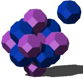
In a simplified form of our construction, we divide the 3d space into cells (see Fig. 1), where only cell surfaces can overlap. We put a 2+1D topological order on each patch of overlapping surfaces. The edges can be viewed as a boundary of several stacked 2+1D topological orders. We put a gapped boundary (a 1+1D anomalous topological orderWen 2013; Kong and Wen 2014; Kapustin 2014b) on each edge. We refer to the constructed gapped states as cellular topological states, to stress the intrinsic cellular structure (such as foliation structureZeng and Wen 2015; Shirley et al. 2018; Shirley et al. 2019) in those gapped states. In general, cellular topological states are gapped non-liquid states, although some special cellular topological states can be liquid states (i.e. the cellular structure disappears).
Our construction is similar to some constructions of SPT and SET phasesChen et al. 2014; Song et al. 2017; Huang et al. 2017; Song et al. 2018. It is also similar to the layer, cage-net, or string-membrane constructions of fracton phasesMa et al. 2017; Slagle and Kim 2017; Vijay 2017; Prem et al. 2019; Slagle et al. 2019; Fuji 2019. However, there are some important differences, which allow us to construct new fracton states with fractal excitations,Haah 2011 even starting from 2+1D topological order.
We like to mention that there are also gapless non-liquid phases. They include Fermi liquid in 2+1D and above,Swingle and McGreevy 2016 as well as some models with emergent graviton-like excitations.Xu 2006; Gu and Wen 2006; Gu and Wen 2012
II A simple construction
II.1 The construction
We first consider a very simple decomposition of the 3d space into hexagonal column’s , where are non-overlaping hexagons whose union form the - plane. (see Fig. 2). We use to label the vertices and the links of honeycomb lattice in the - plane. We then, put bosonic topological orders without symmetry on the faces of hexagonal column’s .
We note that the vertical line at the vertex of the honeycomb lattice is the boundary of the topological order . (Here is the topological order obtained by stacking topological orders and .) So in general, we can put a 1+1D anomalous topological orderWen 2013; Kong and Wen 2014; Kapustin 2014b on the vertical line which is described by a fusion category Lan and Wen 2014. Those fusion categories satisfy
| (1) |
which means that 1+1D anomalous topological order is a gapped boundary of 2+1D topological order or Kong and Wen 2014; Lan et al. 2015; Hu et al. 2017; Lan et al. 2019. Here is the holographic map that map a boundary anomalous topological order to its unique corresponding bulk topological order.Kong and Wen 2014; Kong et al. 2015; Kong et al. 2017; Kong et al. 2020 is closely related to the Drinfeld center, whose physical calculation is presented in . Also, the bar means the time reversal conjugate.
We see that, using the data , we can construct a 3+1D gapped phases for bosonic systems, which can be a non-liquid gapped phase. In general can be non-Abelian topological orders.
We like to mention that if, for example, has a form
| (2) |
then the layer is not connected to the line at vertex-. Such a layer can shrink to the line at vertex- on the other side (see Fig. 3), and hence can be removed (or correspond to trivial case). Thus we are looking for the so called entangled solutions of eqn. (II.1) that do not have the form (II.1). We also like to mention that the gapped boundaries of a 2+1D topological order can be constructed via anyon condensation and are classified by the Lagrangian algebra of the 2+1D topological order Kapustin and Saulina 2011; Kitaev and Kong 2012; Wang and Wen 2015; Kong 2014; Hung and Wan 2014; Hung and Wan 2015.
II.2 Entanglement structure
To understand the cellular topological state in Fig. 2 better, we like to study the entanglement structure of the cellular topological state. The entanglement structure can be revealed by the renormalization of the state (see Fig. 4). The renormalization is done via a basic deformation step in Fig. 4a, where fusing two boundaries and fusing two boundaries given rise to the same boundary of the four stacked 2+1D topological orders (described by the four outer lines): .
To describe such a deformation step more explicitly, we need a quantitative description of the 2+1D topological order and the 1+1D anomalous topological order . The topological orders can be characterized by the representations of mapping class groups for all Riemannian surfaces.Wen 1990; Keski-Vakkuri and Wen 1993 Here for simplicity,Mignard and Schauenburg 2017; Bonderson et al. 2018; Wen and Wen 2019 we will only use the representation for mapping class group of a torus.Rowell et al. 2009; Wen 2015 In other words, we will use the matrices (the generators of a modular representation of ) to characterize a 2+1D topological order , where label the types of the topological excitations in the topological order. Similarly, the gapped domain walls between two topological orders characterized by and are characterized by the wave function overlap of the degenerate ground states, and , of the two topological orders on torus:Lan et al. 2019
| (3) |
where is local hermitian operator like a Hamiltonian of a quantum system, is the area of the torus and is a topological invariant that characterize the domain between the two topological orders. turns out to be non-negative integers for torus, which satisfyLan et al. 2015; Lan et al. 2019
| (4) |
where and are the fusion coefficients for the topological excitations in the two topological orders.
Now let us describe an elementary deformation step. Consider three topological orders , and characterized by , , and . A tensor describes a domain wall between and , and a tensor describes a domain wall between and . The two domain wall and can fuse into a single domain wall (see Fig. 5a):
| (5) |
Note the and are fused with a “glue” (see Fig. 5)Kong et al. 2015; Kong et al. 2017, which is indicated by the subscript of . It turns out that the domain wall is characterized by a tensor
| (6) |
The above just describes the composition of wavefunction overlap in Fig. 5b.
We note that the above elementary step is reversible, which can fuse two domain walls or split a single domain wall. A fusion followed a split in a different direction produces the elementary deformation step in Fig. 4a.
If one side of the domain wall between and is trivial (say is trivial), then the domain wall (i.e. the boundary of ) is described by (or by if the boundary is at the opposite side of , where corresponds to the trivial excitation). We see that the boundary in our construction (see Fig. 2) is characterized by non-negative integer tensor
| (7) |
where labels the topological excitations in and labels the topological excitations in etc .
The above discussion suggests that we can view the blue honeycomb lattice in Fig. 4 as a tensor network, where the tensors at the solid-blue vertices are given by , while the tensors at the open-blue vertices are given by . The link carries the index which label the types of topological excitations in . The trace of the tensor network give us the partition function, which is the ground state degeneracy of the cellular topological state.Wang and Wen 2015; Lan et al. 2015; Lan et al. 2019
To see why trace of tensor network give rise to ground state degeneracy, let us consider a simple tensor network with two vertices connected by a linkWang and Wen 2015; Lan et al. 2015. The link corresponds to a topological order (i.e. the 2+1D gauge theory)Read and Sachdev 1991; Wen 1991. The topological order has four type of topological excitations , labeled by respectively. The modular matrices are given by
| (8) |
The topological order has two gapped boundayies: from -particle condensation and from -particle condensationKitaev and Kong 2012. There are described by the following rank-1 tensors ()
| (9) |
If both boundaries in Fig. 6 are given by , then the ground state degeneracy of the system is given by . This result can also be obtained using the -string operator that creates a pairs of -particle at its ends, and the -string operator that creates a pairs of -particle at its ends. Since -particles condense at the boundaries, the open -string operator, , connecting the two boundaries does change the energy (i.e. commute with the Hamiltonian). A loop of the -string operator in -direction, , also commute with the Hamiltonian. Since the -string operator and the -string operator intersect at one point and anti-commute , the ground states are 2-fold degenerate.
If the boundaries in Fig. 6 are given by and , then the ground state degeneracy of the system is given by . In this case, there is no string operators that connect the two boundaries and create two condensing particles.
With the above tensor representation of the boundaries, the renormalization of the cellular topological state becomes the standard renormalization of tensor network.Verstraete and Cirac 2004; Levin and Nave 2007 Let us assume that, in the hexagonal tensor network (see Fig. 2 and 4b), all are the same , whose topological excitations are labeled by . The boundaries at the solid-bule vertices are given by (or by tensor ), while boundaries at the open-bule vertices are given by (or by tensor ). For simplicity, we will assume
| (10) |
Then, the deformation in Fig. 4a is explicitly given by the following tensor relation:
| (11) |
where label the topological excitations in a new 2+1D topological order . We like to mention that the deformation (11) is not unique. There can be many choices of that satisfy eqn. (11). We like to find the deformation where has minimal total quantum dimension . Here is the quantum dimensions of topological excitations in . Later, we will see that if the resulting is trivial or equal to the original , then the corresponding cellular topological state may be a liquid state.
We like to remark that, as we will see later, a cellular state contains extra local structures that are not related to the universal class of a gapped state. So, by choosing to have minimal total quantum dimension, we hope to obtain the simplest cellular topological state after each step of renormalization, trying to remove those local structures as much as possible.
We can use the deformation Fig. 4a to deform the blue hexagonal tensor network in Fig. 4b to the one described by red links in Fig. 4b. We then shrink the small triangles in Fig. 4b to a point and obtain a new red hexagonal tensor network in Fig. 4c. The new boundaries and are given by
| (12) |
The two relations (11) and (II.2) define the renormalization of the cellular topological state.
III Cellular topological states from 2+1D topological order
III.1 A general construction
In this section, we are going to construct some simple cellular topological states in Fig. 2 by choosing to be the same 2+1D topological order . We find that has 10 types of gapped boundaries, , that are entangled (i.e. do not have the form in eqn. (II.1)). Their tensor representations, , are givein by (only non-zero elements are listed):
| (13) |
The first four, , are cyclic symmetric (10). Let us examine those four types of the boundaries of in more details. First we note that and as well as and differ by an automorphism of the topological order: , where labels the three topological orders in . Those boundaries are formed by condensing the topological excitations in the three topological ordersKitaev and Kong 2012; Kong 2014; Hung and Wan 2014; Hung and Wan 2015. In the following, we list the condensing excitations (the generators) for the four boundaries:
| (14) |
which are obtained from the tensor indices with .
If we assume to be the trival topological order, then the equation eqn. (11) for the deformation in Fig. 11a has no solutions, for those cyclic symmetric boundaries. If we assume to be given by the 2+1D topological order , then for the following ’s
| (15) |
the deformation eqn. (11) also has no solution. But, for other cyclic symmetric boundaries ’s, the deformation eqn. (11) has two solutions, which are given by (see Fig. 11)
| (16) |
If we choose to be a more general topological order, such as , then eqn. (11) always has solutions (see Fig. 7).
After obtaining and , we can perform the shrinking operation (II.2) (see Fig. 4) to obtain :
| (17) |
Here means that the boundary is formed by accidentally degenerate and . Since comes from fusing three ’s. We roughly have a fusion rule for the boundaries: . The results (III.1) suggest that the boundary and have a quantum dimension . So the ground state degeneracy is roughly given by (up to a finite factor), where and are the number of type-A and type-B vertices (see Fig. 2). In other words the ground state degeneracy is roughly given by where is the number of the hexagons (see Fig. 2).
In our above discussions, we have assumed that the vertices in the honeycomb lattice (see Fig. 2) is far apart. This leads to the accidentally degeneracy of two ’s. However, in reality, the vertices in the honeycomb lattice have a small separation. In this case, the degeneracy of two ’s is split.
To summarize, we constructed five cellular topological phases labeled by the following ’s:
| (18) |
Those phases have the key properties that under the renormalization in Fig. 4, we cannot reduce the 2+1D topological order to the trivial one, but can be unchanged under renormalization: . Later, we will see that the invariance of under renormalization suggests that the corresponding cellular topological state is a liquid state.
We also constructed five cellular topological phases labeled by the following ’s:
| (19) |
Those phases have the key properties that under the renormalization in Fig. 4, we cannot reduce the 2+1D topological order to the trivial one, and cannot be unchanged under the renormalization. Later, we will see that the non-invariance of under renormalization suggests that the corresponding cellular topological state is a non-liquid state.
III.2 Cellular topological state
Some cellular topological states are non-liquid states, while other cellular topological states are actually liquid states. In this section, we are going to discuss a cellular topological state , and show that it is actually a gapped liquid state – a 3+1D topological ordered state described by gauge theory.
The cellular topological state is constructed using 2+1D topological order, and choosing the junction of three topological orders to be the 1+1D anomalous topological order in eqn. (III.1) (see Fig. 2).
The 1+1D topological order has a condensation of , , and , for the excisions in the connected 2+1D topological order. This means that the -particles can freely move between the 2+1D topological orders connected by the 1+1D topological order (see Fig. 8). In other words, the -particle can move freely in the whole 3d space.
From the renormalization of the corresponding tensor network
| (20) |
we find that the ground state degeneracy is roughly given by . Such degeneracy can be understood by using the closed -string operator that move an -particle around a hexagon and the closed -string operators that wraps around in the -direction (see Fig. 6). Both closed string operators commute with the Hamiltonian. Since and anti-commute when they intersects, we find that each hexagon contributes a factor 2 (corresponding to ) to the ground state degeneracy.
The cellular topological state has a tensor network representation (see Fig. 2 and 4). We can also compute ground state state degeneracy using the trace of the tensor network. Each link of the tensor network has a label . The label corresponds to a stripe of topological order in the trivial sector. The label correspond to a stripe in the non-trivial sectors. Applying an open -string operator connecting the two boundaries to the trivial sector produces the sector- (see Fig. 6). Similarly, applying the open -string (-string) operator () connecting the two boundaries to the trivial sector produces the sector- (the sector-).
A ground state of the cellular topological phase is given by the stripes of topological orders, all in the trivial sector (i.e. with label on all links). Now we apply a loop -string operators on some links to make them to be a small loop of sector- (see Fig. 8). The configuration corresponds to another degenerate ground state. Thus each hexagon contributes a factor 2 to the ground state degeneracy.
When the separation between vertices is small, the operators are local operators. We may include such operators in the Hamlitonian . The new Hamiltonian no longer commute with -string operators . So splits the ground state degeneracy. The new ground states is believed to have a finite degeneracy independent of system size.
The condensation at the 1+1D topological order implies that we can create three -particles on the neighboring three 2+1D topological orders, which form a small triangle in the dual honeycomb lattice. Putting many small triangles together gives us a loop in the dual honeycomb lattice formed by the -particles (see Fig. 9). However, the -coordinates of the -particles can be arbitrary.
But if we add the term to the Hamiltonian, it will confine two -particles in the same stripe of the topological order. In this case the above loop of the -particles must have similar -coordinates, in order to reduce the energy.
Those properties suggest that the cellular topological state is a 3+1D topological order . The free-moving -particle is the point-like -charge in . The loop of -particles is the -flux loop in .
III.3 Cellular topological state
The cellular topological state is also a gapped liquid state – a 3+1D topological ordered state described by twisted gauge theory where the point-like -charge is a fermion.Levin and Wen 2003
The 1+1D topological order has a condensation of , , and , for the excitations in the connected 2+1D topological orders. This means that the -particles can freely move between the 2+1D topological orders connected by the 1+1D topological order (see Fig. 10). In other words, the -particle can move freely in the whole 3d space, which corresponds to the point-like -charge in the 3+1D topological order . Similarly, the loop of -particles is the -flux loop in .
III.4 Cellular topological state
The cellular topological state is a gapped non-liquid state, which is a fracton state with fractal excitations. In such a cellular topological state, -particle (-particle) can move across the () boundaries (see Fig. 11). But the motion of -particle (-particle) is blocked by the () boundaries. To move across the () boundaries, the -particle (-particle) must split into two (see Fig. 11). So the - and -particles cannot move freely in - direction, indicating that the cellular topological state maybe a non-liquid state. However, the -particle and -particle can move freely in -direction within a stripe of topological order (see Fig. 9).
Remember that a ground state of the cellular topological phase is given by the stripes of topological orders, all in the trivial sector (i.e. with label on all links). Now we apply the -string operators on some links to make them to be the sector-. The created -particle bound state on a vertex must be able to condense on the boundary. In this case, we create another degenerate ground state (see Fig. 12). We can also apply the -string operators on some links to make them to be the sector-. The created -particle bound state on the boundary must be able to condense on the boundary (the resulting configuration is similar to Fig. 12). This way, we obtain another degenerate ground state. We can also apply the -string and -string operators together to obtain new degenerate ground states. Counting all such configurations give us the ground state degeneracy. We note that different degenerate ground states have a large separation of code distance, which increases with system size.
From Fig. 12, we see that, in the ground state, the links in sector- form many small triangles. A corner of a triangle must connect to one and only one corner of another triangle. This way, the links in sector- form a fractal (see Fig. 12). This implies that the cellular topological state is a fracton state with fractal excitations.
If a corner of a triangle is not connected to any corner triangle, such a corner will represent a point-like excitation. But the - motion for such a point-like excitation is highly restricted, like the point excitations in Haah’s cubic code. Such kind of point excitations are called fractons. We see fractons are created at the corners of the fractal operator. However, fractons can move freely in the -direction within a stripe of topological order.
We believe that the cellular topological states, , , , , are similar to the cellular topological states discussed above. They should also be fracton states with fractal excitations.
III.5 A cellular topological state on square column lattice
In this section we consider a cellular topological state on a lattice formed by square columns (see Fig. 13). The stripes in the -direction are occupied by 2+1D topological order. The red and blue vertical lines are two kinds of boundaries, and , of those topological orders:
| (21) |
The two boundaries are characterized by the following condensing topological excitations (the generators):
| (22) |
From the condensing particles on the boundaries, we see that the -particle can move across the boundaries, while the -particle can move across the boundaries. But, the arrangement of the and boundaries is such that the long distant motion of the - and -particles is blocked and they cannot move freely in the - direction. This suggests the cellular topological state to be a non-liquid state.
If all the links are in sector-1, then we have a minimal energy ground state. If we change some links to sector-3 (marked by in Fig. 13), we will get an excited state. We may group the sector-3 links into small diamonds (see Fig. 13). Only the vertices that touch an odd number of the diamonds cost a finite energy (see Fig. 13), and correspond to a fracton. A fracton cannot move by itself in - directions. Only a pair of fractons can move in a certain way in - directions. But a fracton can move freely and independently in -direction. The fractons are created at the corner of diamond-shaped membrane operators. Those properties suggests that the constructed cellular topological state is a type-I fracton state.
III.6 A cellular topological state on cubic lattice
Now, we consider a cellular topological state on a cubic lattice columns (see Fig. 14), which is a generalization of the square column model in the last section. The square faces of the cubic lattice are occupied by 2+1D topological order. The red, blue, and green lines are three kinds of boundaries, , , and of those topological orders:
| (23) |
The above three boundaries are characterized by the following condensing topological excitations (the generators):
| (24) |
From the condensing particles on the boundaries, we see that the -particle can move across the boundaries, the -particle can move across the boundaries, and the -particle can move across the boundaries. But, the arrangement of the , , and boundaries is such that the long distant motion of the -, -, and -particles is blocked and they cannot move freely in the any directions. In other words, they are localized in a finite region. To move further, those particles must split into more and more particles. This suggests the cellular topological state in Fig. 14 to be a non-liquid state. In particular, the structure described in Fig. 13 also appears in the cubic cellular model, and gives rise to point-like excitations with constrained motion.
IV Reverse renormalization and generic construction
To systematically understand and to classify a gapped liquid state (such as a topologically ordered state), we perform wavefunction renormalization by removing the unentangled degrees of freedom.Verstraete and Cirac 2004; Vidal 2007; Aguado and Vidal 2008; Gu et al. 2008 We hope to obtain a fixed-point wave function which gives us a classifying understanding of the gapped liquid states. We also hope the fixed-point wave function is described by a topological quantum field theory which does not dependent on the lattice details.
However, for gapped non-liquid states, due to their intrinsic foliation or cellular structure, above general approach does not work. In particular, we should not expect to have a quantum field theory to describe a non-liquid state. (But a quantum field theories with explicit layer structure may work.Slagle et al. 2019) On the other hand, we still hope to obtain some kind of fixed-point wave functions for non-liquid states, so that we can have a systematic and classifying understanding of non-liquid states.
Here we like to propose a reverse renormalization approach to obtain the fixed-point wave functions for non-liquid states. In such an approach, we add unentangled degrees of freedom to our systems, to separation the layers in the foliation or cellular structure. After many steps of renormalization, we get 3+1D gapped liquid states between layers (i.e. within a cell), such as topologically ordered states or SET/SPT states if we have symmetry. (In our previous discussions, we have assumed the 3+1D gapped liquid states to be trivial product states.) On the layers, we have 2+1D anomalous topological orders, which are the domain walls separating the neighboring 3+1D topological orders. The layers join at edges, which correspond to 1+1D anomalous topological orders. The edges join at vertices, which correspond to 0+1D anomalous topological orders (see Fig. 1).
The above reverse renomalization understanding of non-liquid states suggests the following general construction. We first decompose the 3d space into cells (see Fig. 1). We assign (possibly different) 3+1D topological orders to the 3d cells, assign 2+1D anomalous topological orders to the 2d surfaces, assign 1+1D anomalous topological orders to the 1d edges, and assign 0+1D anomalous topological orders to the 0d vertices. (Without symmetry, the 0+1D anomalous topological orders are always trivial.Kong and Wen 2014) This is a quite general construction, which may cover all the non-liquid states. However, some constructions may give rise to ground state degeneracies that can be lifted by local operators. We need to include those local operators to lift the degeneracies and to stabilize the constructed states. Also, different constructions may lead to the same gapped non-liquid phase. Finding the equivalence relations between different constructions is an every important issue.
Our construction also works if there are on-site symmetry, by requiring the (anomalous) topological orders in various dimensions to have the same symmetry. In the presence of space group symmetry, we need to choose the cellular structure to have the space group symmetry. We also need to choose (anomalous) topological orders in various dimensions to have the proper symmetries, as discussed in .
After posting this paper, the author became aware of a prior unpublished work (now posted as ) where a very similar construction, based on defect network in a 3+1D topological quantum field theory, was proposed. The defect planes and defect lines correspond to the (anomalous) 2+1D and 1+1D topological orders in this paper. Later, another similar construction was proposed in .
I would like to thank Xie Chen and Kevin Slagle to bring the above work to my attention. This work is motivated by the presentations in the Annual Meeting of Simons Collaboration on Ultra-Quantum Matter, where the issue of the fixed point field theory for fracton phases were discussed. This research was partially supported by NSF DMS-1664412. This work was also partially supported by the Simons Collaboration on Ultra-Quantum Matter, which is a grant from the Simons Foundation (651440).
References
- Landau (1937a) L. D. Landau, Phys. Z. Sowjetunion 11, 26 (1937a).
- Landau (1937b) L. D. Landau, Phys. Z. Sowjetunion 11, 545 (1937b).
- Chen et al. (2010) X. Chen, Z.-C. Gu, and X.-G. Wen, Phys. Rev. B 82, 155138 (2010), arXiv:1004.3835 .
- Zeng and Wen (2015) B. Zeng and X.-G. Wen, Phys. Rev. B 91, 125121 (2015), arXiv:1406.5090 .
- Swingle and McGreevy (2016) B. Swingle and J. McGreevy, Phys. Rev. B 93, 045127 (2016), arXiv:1407.8203 .
- Wen (1989) X. G. Wen, Phys. Rev. B 40, 7387 (1989).
- Wen (1990) X. G. Wen, Int. J. Mod. Phys. B 04, 239 (1990).
- Keski-Vakkuri and Wen (1993) E. Keski-Vakkuri and X.-G. Wen, Int. J. Mod. Phys. B 07, 4227 (1993).
- Wen (2002) X.-G. Wen, Phys. Rev. B 65, 165113 (2002), cond-mat/0107071 .
- Essin and Hermele (2013) A. M. Essin and M. Hermele, Phys. Rev. B 87, 104406 (2013), arXiv:1212.0593 .
- Hung and Wan (2013) L.-Y. Hung and Y. Wan, Phys. Rev. B 87, 195103 (2013), arXiv:1302.2951 .
- Xu (2013) C. Xu, Phys. Rev. B 88, 205137 (2013), arXiv:1307.8131 .
- Mesaros and Ran (2013) A. Mesaros and Y. Ran, Phys. Rev. B 87, 155115 (2013), arXiv:1212.0835 .
- Chen et al. (2015) X. Chen, F. J. Burnell, A. Vishwanath, and L. Fidkowski, Phys. Rev. X 5, 041013 (2015), arXiv:1403.6491 .
- Chang et al. (2015) L. Chang, M. Cheng, S. X. Cui, Y. Hu, W. Jin, R. Movassagh, P. Naaijkens, Z. Wang, and A. Young, J. Phys. A: Math. Theor. 48, 12FT01 (2015), arXiv:1412.6589 .
- Cheng et al. (2017) M. Cheng, Z.-C. Gu, S. Jiang, and Y. Qi, Phys. Rev. B 96, 115107 (2017), arXiv:1606.08482 .
- Heinrich et al. (2016) C. Heinrich, F. Burnell, L. Fidkowski, and M. Levin, Phys. Rev. B 94, 235136 (2016), arXiv:1606.07816 .
- Gu and Wen (2009) Z.-C. Gu and X.-G. Wen, Phys. Rev. B 80, 155131 (2009), arXiv:0903.1069 .
- Chen et al. (2011a) X. Chen, Z.-X. Liu, and X.-G. Wen, Phys. Rev. B 84, 235141 (2011a), arXiv:1106.4752 .
- Chen et al. (2013) X. Chen, Z.-C. Gu, Z.-X. Liu, and X.-G. Wen, Phys. Rev. B 87, 155114 (2013), arXiv:1106.4772 .
- Chamon (2005) C. Chamon, Phys. Rev. Lett. 94, 040402 (2005).
- Haah (2011) J. Haah, Phys. Rev. A 83, 042330 (2011), arXiv:1101.1962 .
- Shirley et al. (2018) W. Shirley, K. Slagle, Z. Wang, and X. Chen, Phys. Rev. X 8, 031051 (2018), arXiv:1712.05892 .
- Shirley et al. (2019) W. Shirley, K. Slagle, and X. Chen, SciPost Phys. 6, 015 (2019), arXiv:1803.10426 .
- Vijay et al. (2016) S. Vijay, J. Haah, and L. Fu, Phys. Rev. B 94, 235157 (2016), arXiv:1603.04442 .
- Chen et al. (2011b) X. Chen, Z.-C. Gu, and X.-G. Wen, Phys. Rev. B 83, 035107 (2011b), arXiv:1008.3745 .
- Schuch et al. (2011) N. Schuch, D. Pérez-García, and I. Cirac, Phys. Rev. B 84, 165139 (2011), arXiv:1010.3732 .
- Barkeshli et al. (2014) M. Barkeshli, P. Bonderson, M. Cheng, and Z. Wang, (2014), arXiv:1410.4540 .
- Lan et al. (2017) T. Lan, L. Kong, and X.-G. Wen, Phys. Rev. B 95, 235140 (2017), arXiv:1602.05946 .
- Lan et al. (2016) T. Lan, L. Kong, and X.-G. Wen, Commun. Math. Phys. 351, 709 (2016), arXiv:1602.05936 .
- Lan et al. (2018) T. Lan, L. Kong, and X.-G. Wen, Phys. Rev. X 8, 021074 (2018), arXiv:1704.04221 .
- Lan and Wen (2019) T. Lan and X.-G. Wen, Phys. Rev. X 9, 021005 (2019), arXiv:1801.08530 .
- Zhu et al. (2019) C. Zhu, T. Lan, and X.-G. Wen, Phys. Rev. B 100, 045105 (2019), arXiv:1808.09394 .
- Kapustin (2014a) A. Kapustin, (2014a), arXiv:1404.6659 .
- Gu and Wen (2014) Z.-C. Gu and X.-G. Wen, Phys. Rev. B 90, 115141 (2014), arXiv:1201.2648 .
- Kapustin et al. (2015) A. Kapustin, R. Thorngren, A. Turzillo, and Z. Wang, J. High Energ. Phys. 2015, 1 (2015), arXiv:1406.7329 .
- Gaiotto and Kapustin (2016) D. Gaiotto and A. Kapustin, Int. J. Mod. Phys. A 31, 1645044 (2016), arXiv:1505.05856 .
- Freed and Hopkins (2016) D. S. Freed and M. J. Hopkins, (2016), arXiv:1604.06527 .
- Kapustin and Thorngren (2017) A. Kapustin and R. Thorngren, J. High Energ. Phys. 2017, 80 (2017), arXiv:1701.08264 .
- Wang and Gu (2018) Q.-R. Wang and Z.-C. Gu, Phys. Rev. X 8, 011055 (2018), arXiv:1703.10937 .
- Pretko et al. (2020) M. Pretko, X. Chen, and Y. You, (2020), arXiv:2001.01722 .
- Kong and Wen (2014) L. Kong and X.-G. Wen, (2014), arXiv:1405.5858 .
- Wen (2013) X.-G. Wen, Phys. Rev. D 88, 045013 (2013), arXiv:1303.1803 .
- Kapustin (2014b) A. Kapustin, (2014b), arXiv:1403.1467 .
- Chen et al. (2014) X. Chen, Y.-M. Lu, and A. Vishwanath, Nat Commun 5, 4507 (2014), arXiv:1303.4301 .
- Song et al. (2017) H. Song, S.-J. Huang, L. Fu, and M. Hermele, Phys. Rev. X 7, 011020 (2017), arXiv:1604.08151 .
- Huang et al. (2017) S.-J. Huang, H. Song, Y.-P. Huang, and M. Hermele, Phys. Rev. B 96, 205106 (2017), arXiv:1705.09243 .
- Song et al. (2018) Z. Song, C. Fang, and Y. Qi, (2018), arXiv:1810.11013 .
- Ma et al. (2017) H. Ma, E. Lake, X. Chen, and M. Hermele, Phys. Rev. B 95 (2017), 10.1103/physrevb.95.245126, arXiv:1701.00747 .
- Slagle and Kim (2017) K. Slagle and Y. B. Kim, Phys. Rev. B 96, 165106 (2017), arXiv:1704.03870 .
- Vijay (2017) S. Vijay, (2017), arXiv:1701.00762 .
- Prem et al. (2019) A. Prem, S.-J. Huang, H. Song, and M. Hermele, Physical Review X 9, 021010 (2019), arXiv:1806.04687 .
- Slagle et al. (2019) K. Slagle, D. Aasen, and D. Williamson, SciPost Physics 6, 043 (2019), arXiv:1812.01613 .
- Fuji (2019) Y. Fuji, Phys. Rev. B 100, 235115 (2019), arXiv:1908.02257 .
- Xu (2006) C. Xu, (2006), cond-mat/0602443 .
- Gu and Wen (2006) Z.-C. Gu and X.-G. Wen, (2006), gr-qc/0606100 .
- Gu and Wen (2012) Z.-C. Gu and X.-G. Wen, Nucl. Phys. B 863, 90 (2012), arXiv:0907.1203 .
- Lan and Wen (2014) T. Lan and X.-G. Wen, Phys. Rev. B 90, 115119 (2014), arXiv:1311.1784 .
- Lan et al. (2015) T. Lan, J. C. Wang, and X.-G. Wen, Phys. Rev. Lett. 114, 076402 (2015), arXiv:1408.6514 .
- Hu et al. (2017) Y. Hu, Y. Wan, and Y.-S. Wu, Chinese Physics Letters 34, 077103 (2017), arXiv:1706.00650 .
- Lan et al. (2019) T. Lan, X. Wen, L. Kong, and X.-G. Wen, (2019), arXiv:1911.08470 .
- Kong et al. (2015) L. Kong, X.-G. Wen, and H. Zheng, (2015), arXiv:1502.01690 .
- Kong et al. (2017) L. Kong, X.-G. Wen, and H. Zheng, Nucl. Phys. B 922, 62 (2017), arXiv:1702.00673 .
- Kong et al. (2020) L. Kong, T. Lan, X.-G. Wen, Z.-H. Zhang, and H. Zheng, (2020), arXiv:2005.14178 .
- Kapustin and Saulina (2011) A. Kapustin and N. Saulina, Nucl. Phys. B 845, 393 (2011), arXiv:1008.0654 .
- Kitaev and Kong (2012) A. Kitaev and L. Kong, Commun. Math. Phys. 313, 351 (2012), arXiv:1104.5047 .
- Wang and Wen (2015) J. C. Wang and X.-G. Wen, Phys. Rev. B 91, 125124 (2015), arXiv:1212.4863 .
- Kong (2014) L. Kong, Nucl. Phys. B 886, 436 (2014), arXiv:1307.8244 .
- Hung and Wan (2014) L.-Y. Hung and Y. Wan, Int. J. Mod. Phys. B 28, 1450172 (2014), arXiv:1308.4673 .
- Hung and Wan (2015) L.-Y. Hung and Y. Wan, Phys. Rev. Lett. 114, 076401 (2015), arXiv:1408.0014 .
- Mignard and Schauenburg (2017) M. Mignard and P. Schauenburg, (2017), arXiv:1708.02796 .
- Bonderson et al. (2018) P. Bonderson, C. Delaney, C. Galindo, E. C. Rowell, A. Tran, and Z. Wang, (2018), arXiv:1805.05736 .
- Wen and Wen (2019) X. Wen and X.-G. Wen, (2019), arXiv:1908.10381 .
- Rowell et al. (2009) E. Rowell, R. Stong, and Z. Wang, Commun. Math. Phys. 292, 343 (2009), arXiv:0712.1377 .
- Wen (2015) X.-G. Wen, Nat. Sci. Rev. 3, 68 (2015), arXiv:1506.05768 .
- Read and Sachdev (1991) N. Read and S. Sachdev, Phys. Rev. Lett. 66, 1773 (1991).
- Wen (1991) X. G. Wen, Phys. Rev. B 44, 2664 (1991).
- Verstraete and Cirac (2004) F. Verstraete and J. I. Cirac, (2004), cond-mat/0407066 .
- Levin and Nave (2007) M. Levin and C. P. Nave, Phys. Rev. Lett. 99, 120601 (2007).
- Levin and Wen (2003) M. Levin and X.-G. Wen, Phys. Rev. B 67, 245316 (2003), cond-mat/0302460 .
- Vidal (2007) G. Vidal, Phys. Rev. Lett. 99, 220405 (2007).
- Aguado and Vidal (2008) M. Aguado and G. Vidal, Phys. Rev. Lett. 100, 070404 (2008).
- Gu et al. (2008) Z.-C. Gu, M. Levin, and X.-G. Wen, Phys. Rev. B 78, 205116 (2008), arXiv:0806.3509 .
- Aasen et al. (2020) D. Aasen, B. Bulmash, A. Prem, K. Slagle, and D. J. Williamson, (2020), arXiv:2002.05166 .
- Wang (2020) J. Wang, (2020), arXiv:2002.12932 .