跳到论文正文
W Papers独立论文阅读器 arXiv:2002.02301 论文正文 计算阅读时间 · 0%
引用这篇论文根据当前论文元数据生成,正式投稿前建议核对。


License: arXiv.org perpetual non-exclusive license
arXiv:2002.02301v1 [cs.IT] 28 Jan 2020

Wireless Powered Protocol Exploiting Energy Harvesting During Cognitive Communications

Anirudh Agarwal       and Deepak Mishra    Thanks: A. Agarwal is with the Department of ECE, The LNM Institute of Information Technology, Jaipur, 302031 India (e-mail: anirudh.agarwal@lnmiit.ac.in Thanks: D. Mishra is with the Department of Electrical Engineering, Linköping University, Linköping, 58183 Sweden (e-mail: deepak.mishra@liu.se).
Abstract

In this letter, a novel wireless powered protocol is proposed to maximize the system throughput of an energy harvesting (EH) based cognitive radio network, while satisfying a minimum primary user rate requirement. For EH, we exploit both dedicated wireless power transfer from primary base station as well as ambient ones available due to wireless information transfer among primary and secondary users. Specifically, we prove convexity of the optimization problem and obtain semi-closed-form for globally optimal solution. Numerical results validate the analysis, and show an average performance improvement of 70%70\% over benchmark scheme for various system parameters.

Index Terms: 
Cognitive radio, energy harvesting, time allocation, sum throughput maximization, wireless power transfer.

I Introduction

Apart from spectrum scarcity, limited battery capacity of low-powered devices poses a major design challenge in 5G wireless communication systems. Cognitive radio (CR) is a promising solution to enhance spectrum utilization efficiency. Moreover, exploiting energy-harvesting (EH) techniques into CR networks (CRNs) has drawn wide attention due to ability of radio frequency (RF) signals to simultaneously carry energy as well as information. This enables better energy sustainability to both primary user (PU) and secondary user (SU) nodes, enhancing quality of service (QoS) in a CR network [1].

In [2], SUs first harvest energy from PU and then forward the primary data after amplification, while PU releases a portion of its time slot to SU in return. In [3], wireless power transfer (WPT) from PU to a pair of SUs has been considered, and the problem of optimal time allocation (TA) has been solved while satisfying a constraint on outage probability of PU system. A joint power control and TA problem has been studied in [4] for maximizing the SU throughput with a limiting interference constraint. However, one common limitation of [2, 3, 4] is that they have not considered a minimum average achievable rate requirement of PU. Shreshta et al. [5] did put a PU throughput constraint, but no closed-form expression was found for global optimal solution for TA, rather they obtained them numerically. Moreover, all the above works have either considered EH by SU from PU or EH by PU from SU, along with EH from primary base station (PBS).

Refer to caption
Fig. 1: An EH-based CR system model with WPT and WIT.

In this work, for better utilization efficiency of harvested energy, we have exploited all EH possibilities, i.e. EH via dedicated WPT from PBS and EH via ambient interference due to wireless information transfer (WIT) between every transmitter-receiver pair. This framework may be practically applicable to battery-constrained self-sustainable communication networks with CR [10]. Further, our optimal designs are targeted for serving applications with the overall system-centric goal, rather than individual node-level, where the best-effort delivery is desired to maximize the aggregate system throughput. To the best of our knowledge, this novel CR framework exploiting all RF-EH possibilities, along with minimum PU throughput constraint, has not been investigated earlier. Key contributions of this work are: 1) A novel timing protocol is proposed with all RF-EH possibilities. 2) Convexity of optimization problem to maximize system throughput subject to a minimum PU rate constraint is proved. 3) Semi-closed-form globally optimal TA solution is obtained. 4) Improved performance of proposed scheme over benchmark and uniform TA schemes is numerically demonstrated with nontrivial optimal design insights.

II Proposed Transmission Protocol

We consider an EH-based interweave CR system with nodes scattered over a square field of length LL meters (m), as shown in Fig. 1. It consists of a PBS at the center, a pair of primary transmitter P​UTPU^{T} and receiver P​URPU^{R}, and NN pairs of secondary transmitters SjTS^{T}_{j} and receivers SjRS^{R}_{j}, j∈𝒩Nj\in\mathcal{N}_{N}, where 𝒩N≜{1,2,…​N}\mathcal{N}_{N}\triangleq\{1,2,...N\}. PBS is assumed to be constantly powered by a source. Each PU and SU transmitter-receiver (TR) pair exhibits EH capabilities and is composed of a single omnidirectional antenna. The channel links between any two TR pairs are assumed to suffer from path-loss. Considering channel reciprocity, the channel power gains of the links from PBS to P​URPU^{R}, PBS to SjRS^{R}_{j}, P​UTPU^{T} to SjRS^{R}_{j}, and SjTS^{T}_{j} to SkRS^{R}_{k}, are respectively denoted by GB​PG_{BP}, GB​SjG_{BS_{j}}, GP​SjG_{PS_{j}} and GSj​SkG_{S_{j}S_{k}}, ∀j,k∈𝒩N\forall j,k\in\mathcal{N}_{N}. Here, we have assumed perfect channel knowledge for each communication link [6] with no external ambient EH source.

Refer to caption
Fig. 2: Proposed RF powered protocol for cognitive EH network.

In Fig. 2, the proposed novel timing protocol is depicted in which a 3-phase approach is followed for WPT and WIT. The time for WPT and WIT has been allocated orthogonally over a unit slot duration (T=1T=1 sec). The optimization of TA for WPT and WIT is performed by the PBS on slot-by-slot basis. Further, we assume that each node is equipped with its own battery having sufficient stored energy in it, which if consumed, will be replenished later via ambient EH due to WIT in subsequent phases within a slot. So, the energy remains conserved in a slot. To be specific, in Phase-1, PBS transfers power wirelessly to PU and SUs for τ0\tau_{0} duration. In Phase-2 of τ1\tau_{1} duration, P​UTPU^{T} can utilize its battery power for data transmission (DT), and SUs can harvest energy from P​UT{PU}^{T}-P​UR{PU}^{R} WIT. Similarly, every SU can consume its battery power for DT in their respective subphase of τj\tau_{j} duration in Phase-3, ∀j∈{2,3,…​N+1}\forall j\in\{2,3,...N+1\}. Whereas, PU can recharge its battery back during Phase-3 via EH due to the undergoing WIT between SjTS^{T}_{j} and SjRS^{R}_{j}, ∀j∈𝒩N\forall j\in\mathcal{N}_{N}. Likewise, every SU can transfer back its consumed power to its respective battery before the slots end, by EH during other nodes’ DT phases.

For WPT, with P0P_{0} being the transmit power of PBS, energy harvested by PU from PBS over τ0\tau_{0} duration is given by,

EB​Ph=η​P0​GB​P​τ0.E^{h}_{BP}=\eta P_{0}G_{BP}\tau_{0}. (1)

where η∈(0,1)\eta\in(0,1) is the rectification efficiency. Similarly, EB​Sjh≜η​P0​GB​Sj​τ0E^{h}_{BS_{j}}\hskip-1.42262pt\triangleq\hskip-1.42262pt\eta P_{0}G_{BS_{j}}\hskip-1.42262pt\tau_{0}, ∀j∈𝒩N\forall j\hskip-1.42262pt\in\hskip-1.42262pt\mathcal{N}_{N}, is the harvested energy by jt​hj^{th} SU from PBS. Now, PU and SUs can further harvest ambient energy from each others WIT. Consequently, the power received by PU from jt​hj^{th} SU, and that by jt​hj^{th} SU from PU, can be respectively calculated as PSj​PR=EB​Sjh​GP​SjτjP^{R}_{S_{j}P}\hskip-1.42262pt=\hskip-1.42262pt\frac{E^{h}_{BS_{j}}G_{PS_{j}}}{\tau_{j}}, PP​SjR=EB​Ph​GP​Sjτ1P^{R}_{PS_{j}}\hskip-1.42262pt=\hskip-1.42262pt\frac{E^{h}_{BP}G_{PS_{j}}}{\tau_{1}}. Moreover, jt​hj^{th} SU receives PSk​SjR≜EB​Skh​GSk​SjτkP^{R}_{S_{k}S_{j}}\hskip-1.42262pt\triangleq\hskip-1.42262pt\frac{E^{h}_{BS_{k}}G_{S_{k}S_{j}}}{\tau_{k}} power from the kt​hk^{th} SU, ∀j,k∈𝒩N\forall j,k\hskip-1.42262pt\in\hskip-1.42262pt\mathcal{N}_{N}, k≠jk\hskip-1.42262pt\neq\hskip-1.42262ptj. So, overall respective harvested energies for PU and SU DT are:

EPh=EB​Ph+∑j=1NPSj​PR​τ1,\displaystyle E^{h}_{P}=E^{h}_{BP}+\sum_{j=1}^{N}P^{R}_{S_{j}P}\tau_{1}, (2a)
ESjh=EB​Sjh+PP​SjR​τj+∑k∈𝒩Nk≠jPSk​SjR​τj.\displaystyle E^{h}_{S_{j}}=E^{h}_{BS_{j}}+P^{R}_{PS_{j}}\tau_{j}+\sum_{\begin{subarray}{c}k\in\mathcal{N}_{N}\end{subarray}}^{k\neq j}P^{R}_{S_{k}S_{j}}\tau_{j}. (2b)

Therefore, the PU throughput R1R_{1} and SU throughput Rj+1​∀j∈𝒩NR_{j+1}\forall j\in\mathcal{N}_{N} are defined as,

Ri=τi​[log2⁡(1+γi​τ0τi)],\hskip-5.69054ptR_{i}\hskip-1.42262pt=\hskip-1.42262pt\tau_{i}\hskip-1.42262pt\left[\log_{2}\hskip-1.42262pt\left(\hskip-1.42262pt1\hskip-1.42262pt+\hskip-1.42262pt\frac{\gamma_{i}\tau_{0}}{\tau_{i}}\hskip-1.42262pt\right)\hskip-1.42262pt\right]\hskip-1.42262pt, (3)

where i∈𝒩1≜𝒩N∪{N+1}i\hskip-1.42262pt\in\hskip-1.42262pt\mathcal{N}_{1}\triangleq\mathcal{N}_{N}\cup\{N+1\}, γ1=EPh​GB​Pτ0​σ2\gamma_{1}\hskip-1.42262pt=\hskip-1.42262pt\frac{E^{h}_{P}G_{BP}}{\tau_{0}\,\sigma^{2}}, γj+1=ESjh​GSj​Sjτ0​σ2\gamma_{j+1}\hskip-1.42262pt=\hskip-1.42262pt\frac{E^{h}_{S_{j}}\,G_{S_{j}S_{j}}}{\tau_{0}\,\sigma^{2}} ∀j∈𝒩N\forall j\in\mathcal{N}_{N}, and σ2\sigma^{2} is the variance of received zero mean additive white Gaussian noise. Now, from (3), the system throughput Rs​u​mR_{sum} is defined as, Rs​u​m=∑i=1N+1RiR_{sum}\hskip-1.42262pt=\hskip-1.42262pt\sum_{i=1}^{N+1}\hskip-1.42262ptR_{i}. Note that we have considered normalized bandwidth, so spectral efficiency has been defined in terms of throughput.

III Problem Definition

III-A Mathematical Formulation

To maximize Rs​u​mR_{sum} while guaranteeing a minimum PU rate requirement δ\delta, the following problem has to be solved:

(ℙ):max𝝉Rs​u​m,subject toC​1:R1≥δ,C​2:0≤τk≤1,C​3:∑k=1N+1τk≤1,\begin{aligned} \text{($\bm{\mathbb{P}}$)}\hskip-2.84526pt:\hskip 2.84526pt&\underset{\bm{\tau}}{\text{max}}&&\hskip-56.9055ptR_{sum},&\hskip-128.0374pt\text{subject to}&&C1\hskip-1.42262pt:R_{1}\geq\delta,\\ &\hskip 0.0ptC2\hskip-1.42262pt:0\leq\tau_{k}\leq 1,&&\hskip 25.60747ptC3\hskip-1.42262pt:\sum_{k=1}^{N+1}\tau_{k}\leq 1,\end{aligned}
where​𝝉=[τ0​τ1​τ2​…​τN+1]\text{where}\hskip 1.42262pt\bm{\tau}\hskip-1.42262pt=\hskip-1.42262pt\left[\tau_{0}\,\,\tau_{1}\,\,\tau_{2}\,...\,\tau_{N+1}\right]. Keeping boundary constraint C​2C2 implicit, the Lagrangian of (ℙ\bm{\mathbb{P}}) is given by,

ℒ⁡(𝝉,μ1,μ2)=Rs​u​m−μ1​(δ−R1)−μ2​(∑k=0N+1τk−1)\displaystyle\hskip-8.53581pt\mathcal{L}(\bm{\tau},\mu_{1},\mu_{2})=R_{sum}-\mu_{1}(\delta-R_{1})-\mu_{2}\left(\sum_{k=0}^{N+1}{\tau_{k}}-1\right) (4)

where μ1\mu_{1} and μ2\mu_{2} are the non-negative Lagrange multipliers associated with constraints C​1C1 and C​3C3 respectively.

III-B Proof for Convexity of (ℙ)\bm{(}\mathbb{P}\bm{)}

Here we provide Lemmas 1 and 2 for completing this proof.

Lemma 1

The objective Rs​u​mR_{sum} is a concave function of 𝛕\bm{\tau}.

Proof:

The Hessian 𝐇⁡(R​i)\mathbf{H}(Ri) of RiR_{i} defined in (3), ∀i∈𝒩1\forall i\in\mathcal{N}_{1} is a square matrix of order (N+1N+1). So, the Hm​n(i)H^{(i)}_{mn}th element of 𝑯⁡(Ri)\bm{H}\hskip-1.42262pt\left(\hskip-1.42262ptR_{i}\hskip-1.42262pt\right) at mt​hm^{th} row, nt​hn^{th} column, ∀m,n∈𝒩1\forall m,n\in\mathcal{N}_{1} is given by:

Hm​n(i)=Hn​m(i)={∂2Ri∂τm​∂τn=γi2​τ0​τi−2​ωi−2;m≠n, m=i, n=1,∂2Ri∂τm2=−γi2​τi−1​ωi−2;m=n=1,∂2Ri∂τm2=−γi2​τ02​τi−3​ωi−2;m=n=i≥2,0;otherwise,\displaystyle H^{(i)}_{mn}\hskip-1.42262pt=\hskip-1.42262ptH^{(i)}_{nm}\hskip-1.42262pt=\hskip-1.42262pt\begin{cases}\hskip-1.42262pt\frac{\partial^{2}\hskip-1.42262ptR_{i}}{\partial\tau_{m}\partial\tau_{n}}\hskip-1.42262pt=\hskip-1.42262pt\gamma^{2}_{i}\tau_{0}\tau^{-2}_{i}\omega^{-2}_{i}\hskip-1.42262pt;&\hskip-4.2679pt\text{$\hskip-1.42262ptm\hskip-1.42262pt\neq n$, $\hskip-1.42262ptm\hskip-1.42262pt=\hskip-1.42262pti$, $\hskip-1.42262ptn\hskip-1.42262pt=\hskip-1.42262pt1\hskip-1.42262pt$},\\ \hskip-1.42262pt\frac{\partial^{2}\hskip-1.42262ptR_{i}}{\partial\tau^{2}_{m}}\hskip-1.42262pt=\hskip-1.42262pt-\gamma^{2}_{i}\tau^{-1}_{i}\omega^{-2}_{i}\hskip 9.95845pt\,;&\hskip-4.2679pt\text{$m\hskip-1.42262pt=\hskip-1.42262ptn\hskip-1.42262pt=\hskip-1.42262pt1$},\\ \hskip-1.42262pt\frac{\partial^{2}\hskip-1.42262ptR_{i}}{\partial\tau^{2}_{m}}\hskip-1.42262pt=\hskip-1.42262pt-\gamma^{2}_{i}\tau^{2}_{0}\tau^{-3}_{i}\omega^{-2}_{i}\,;&\hskip-4.2679pt\text{$m\hskip-1.42262pt=\hskip-1.42262ptn\hskip-1.42262pt=\hskip-1.42262pti\geq 2$},\\ \hskip 42.67912pt0\hskip 42.67912pt;&\hskip-4.2679pt\text{otherwise},\end{cases}\hskip-19.91692pt (5)

where ωi≜1+γi​τ0τi\omega_{i}\triangleq 1+\frac{\gamma_{i}\tau_{0}}{\tau_{i}}. From (5), it can be clearly seen that all the diagonal entries of 𝑯⁡(Ri)\bm{H}\hskip-1.42262pt\left(\hskip-1.42262ptR_{i}\hskip-1.42262pt\right) are non-positive. Additionally, the determinants of all the odd principal minors of 𝑯⁡(Ri)\bm{H}\hskip-1.42262pt\left(\hskip-1.42262ptR_{i}\hskip-1.42262pt\right) are non-positive and that of even principal minors are non-negative. Therefore, 𝑯⁡(Ri)\bm{H}\hskip-1.42262pt\left(\hskip-1.42262ptR_{i}\hskip-1.42262pt\right) is a negative semi-definite matrix, and RiR_{i} is a concave function of 𝝉\bm{\tau} [7]. Moreover, as the sum of concave functions is also a concave function [7], Rs​u​mR_{sum} is thus proved to be a concave function of 𝝉\bm{\tau}. ∎

Lemma 2

Constraints C​1C1, C​2C2, C​3C3 are convex sets.

Proof:

The Hessian matrix of Rc​o​nP≜δ−R1R^{P}_{con}\triangleq\delta-R_{1}, 𝑯^​(Rc​o​nP)\widehat{\bm{H}}\left(R^{P}_{con}\right) is given by: 𝑯^​(Rc​o​nP)=[∂2Rc​o​nP∂τ02∂2Rc​o​nP∂τ0​∂τ1∂2Rc​o​nP∂τ1​∂τ0∂2Rc​o​nP∂τ12],\hskip-1.42262pt\widehat{\bm{H}}\left(\hskip-1.42262ptR^{P}_{con}\hskip-1.42262pt\right)\hskip-2.84526pt=\hskip-2.84526pt\left[\hskip-2.84526pt\begin{array}[]{ccc}\hskip-1.42262pt\frac{\hskip-1.42262pt\partial^{2}\hskip-1.42262ptR^{P}_{con}\hskip-1.42262pt}{\partial\tau_{0}^{2}}&\frac{\partial^{2}\hskip-1.42262ptR^{P}_{con}}{\partial{\tau_{0}}\partial{\tau_{1}}}\\ \hskip-1.42262pt\frac{\hskip-1.42262pt\partial^{2}\hskip-1.42262ptR^{P}_{con}\hskip-1.42262pt}{\partial{\tau_{1}}\partial{\tau_{0}}}&\frac{\hskip-1.42262pt\partial^{2}\hskip-1.42262ptR^{P}_{con}\hskip-1.42262pt}{\partial\tau_{1}^{2}}\end{array}\hskip-4.2679pt\right]\hskip-2.84526pt, where ∂2Rc​o​nP∂τ02=γ12τ1​ω12\frac{\hskip-1.42262pt\partial^{2}\hskip-1.42262ptR^{P}_{con}\hskip-1.42262pt}{\partial\tau_{0}^{2}}\hskip-2.84526pt=\hskip-2.84526pt\frac{\hskip-1.42262pt\gamma_{1}^{2}\hskip-1.42262pt}{\tau_{1}\omega_{1}^{2}\hskip-1.42262pt}, ∂2Rc​o​nP∂τ0​∂τ1=∂2Rc​o​nP∂τ1​∂τ0=−γ12​τ0τ12​ω12\frac{\partial^{2}\hskip-1.42262ptR^{P}_{con}}{\partial{\tau_{0}}\partial{\tau_{1}}}\hskip-2.84526pt=\hskip-2.84526pt\frac{\partial^{2}\hskip-1.42262ptR^{P}_{con}}{\partial{\tau_{1}}\partial{\tau_{0}}}\hskip-2.84526pt=\hskip-2.84526pt\frac{-\gamma_{1}^{2}\tau_{0}}{\hskip-1.42262pt\tau_{1}^{2}\omega_{1}^{2}}, ∂2Rc​o​nP∂τ12=1τ13​γ12​τ02ω12\frac{\hskip-1.42262pt\partial^{2}\hskip-1.42262ptR^{P}_{con}}{\hskip-1.42262pt\partial{\tau_{1}}^{2}}\hskip-2.84526pt=\hskip-2.84526pt\frac{1}{\tau_{1}^{3}}\frac{\hskip-1.42262pt\gamma_{1}^{2}\tau_{0}^{2}}{\hskip-1.42262pt\omega_{1}^{2}}. So, it can be easily observed that ∂2Rc​o​nP∂τ02,∂2Rc​o​nP∂τ12>0\frac{\hskip-1.42262pt\partial^{2}\hskip-1.42262ptR^{P}_{con}\hskip-1.42262pt}{\partial\tau_{0}^{2}},\frac{\hskip-1.42262pt\partial^{2}\hskip-1.42262ptR^{P}_{con}\hskip-1.42262pt}{\partial\tau_{1}^{2}}\hskip-2.84526pt>\hskip-2.84526pt0 and determinant of 𝑯^​(Rc​o​nP)\widehat{\bm{H}}\left(R^{P}_{con}\right) is zero. This proves that 𝑯^​(Rc​o​nP)\widehat{\bm{H}}\left(R^{P}_{con}\right) is positive semi-definite. Hence Rc​o​nPR^{P}_{con} is a convex function of 𝝉\bm{\tau} [7]. Further, constraints C​2,C​3C2,C3 are linear in 𝝉\bm{\tau}, therefore form convex sets. ∎

IV Globally-Optimal TA Solution

As (ℙ\bm{\mathbb{P}}) is a convex optimization problem, the underlying Karush-Kuhn-Tucker (KKT) point (τk∗,\tau^{*}_{k}, μ1∗,\mu^{*}_{1}, μ2∗\mu^{*}_{2}) ∀k∈𝒩0≜𝒩1∪{0}\forall k\in\mathcal{N}_{0}\triangleq\mathcal{N}_{1}\cup\{0\}, provides the globally-optimal solution of (ℙ\bm{\mathbb{P}}) [7]. The corresponding KKT conditions are,

∂ℒ∂τk=0,∀k∈𝒩0,\displaystyle\frac{\partial\mathcal{L}}{\partial\tau_{k}}=0,\forall k\in\mathcal{N}_{0}, (6a)
μ1​(δ−R1)=0,\displaystyle\mu_{1}(\delta-R_{1})=0, (6b)
μ2​(∑k∈𝒩0τk−1)=0.\displaystyle\textstyle\mu_{2}\left(\sum_{k\in\mathcal{N}_{0}}{\tau_{k}}-1\right)=0. (6c)

Since the highest sum throughput can be obtained only by fully utilizing the available time resource, constraint C​3C3 has to be satisfied at equality by the optimal solution, resulting into μ2∗>0\mu^{*}_{2}>0. Therefore from (6c),

∑k=1N+1τk=1−τ0.\textstyle\sum_{k=1}^{N+1}\;\tau_{k}=1-\tau_{0}. (7)

As μi∗≥0\mu^{*}_{i}\geq 0, ∀i∈{1,2}\forall i\in\{1,2\}, we next consider 22 cases, i.e., unconstrained (μ1∗=0\mu^{*}_{1}=0) and constrained (μ1∗>0\mu^{*}_{1}>0) optimization problems with Rs​u​mR_{sum} as objective and C​1C1 as constraint.

IV-A Unconstrained Rs​u​mR_{sum} Maximization

For μ1∗=0\mu^{*}_{1}=0, we solve (3) and (6a) to get,

∑j=1N+1γj1+γj​τ0∗τj∗=μ2∗​ln⁡2,\displaystyle\sum\limits_{j=1}^{N+1}\frac{\gamma_{j}}{1+\frac{\gamma_{j}\tau^{*}_{0}}{\tau^{*}_{j}}}=\mu^{*}_{2}\ln{2}, (8)
Φ⁡(γk​τ0∗τk∗)=μ2∗​ln⁡2,∀k∈𝒩1,\displaystyle\Phi\hskip-1.42262pt\left(\hskip-1.42262pt\frac{\gamma_{k}\tau^{*}_{0}}{\tau^{*}_{k}}\hskip-1.42262pt\right)\hskip-1.42262pt=\hskip-1.42262pt\mu^{*}_{2}\ln{2},\,\,\,\forall\,\,k\in\mathcal{N}_{1}, (9)

where Φ⁡(x)≜ln⁡(1+x)−x1+x\Phi(x)\triangleq\ln{\left(\hskip-1.42262pt1\hskip-1.42262pt+\hskip-1.42262ptx\right)}\hskip-1.42262pt-\hskip-1.42262pt\frac{x}{1+x}. As Φ⁡(x)\Phi(x) is increasing in xx, if Φ⁡(x1)=Φ⁡(x2)\Phi(x_{1})=\Phi(x_{2}), then x1=x2x_{1}=x_{2}, ∀\forall x1,x2>0x_{1},x_{2}>0. Thus, from (9),

γ1τ1∗=γ2τ2∗=…=γN+1τ(N+1)∗≜Ka.\displaystyle\frac{\gamma_{1}}{\tau^{*}_{1}}=\frac{\gamma_{2}}{\tau^{*}_{{2}}}=...=\frac{\gamma_{N+1}}{\tau^{*}_{(N+1)}}\triangleq K_{a}. (10)

Now with Γa≜∑k=1N+1γk\Gamma_{a}\triangleq\sum_{k=1}^{N+1}\gamma_{k}, from (8), (9) and (10), we have

Φ⁡(Ka​τ0∗)=Γa1+Ka​τ0∗,\displaystyle\Phi\left(K_{a}\tau^{*}_{0}\right)=\frac{\Gamma_{a}}{1+K_{a}\tau^{*}_{0}}, (11)

After few mathematical arrangements, (11) reduces to,

1+Ka​τ0∗=Γa−1𝒲⁡(Γa−1exp⁡[1])≜f⁡(Γa),1+K_{a}\tau^{*}_{0}=\frac{\Gamma_{a}-1}{\mathcal{W}\left(\frac{\Gamma_{a}-1}{\exp[1]}\right)}\triangleq f(\Gamma_{a}), (12)

where 𝒲(.)\mathcal{W}(.) denotes the Lambert W function [8]. So, from (8) and (12), we obtain μ2∗=μ2​a≜Γa(ln⁡2)​f​(Γa)\mu^{*}_{2}=\mu_{2a}\triangleq\frac{\Gamma_{a}}{(\ln{2})f\hskip-1.42262pt\left(\Gamma_{a}\right)}.

Additionally, from (7) and (10), Ka=Γa(1−τ0∗)K_{a}=\frac{\Gamma_{a}}{(1-\tau^{*}_{0})}, which after substituting into (12) will give,

τ0∗=τ0​a≜f⁡(Γa)−1Γa+f⁡(Γa)−1.\tau^{*}_{0}=\tau_{0a}\triangleq\frac{f(\Gamma_{a})-1}{\Gamma_{a}+f(\Gamma_{a})-1}. (13)

Next, (10) and (13) can be solved to find τk∗=τk​a\tau^{*}_{k}=\tau_{ka} as below,

τk​a≜γkΓa+f⁡(Γa)−1,∀k∈𝒩1.\tau_{ka}\triangleq\frac{\gamma_{k}}{{\Gamma_{a}+f(\Gamma_{a})-1}},\forall k\in\mathcal{N}_{1}. (14)

So, if R1>δR_{1}\hskip-1.42262pt>\hskip-1.42262pt\delta, then (τk∗=τk​a,\tau^{*}_{k}\hskip-1.42262pt=\hskip-1.42262pt\tau_{ka}, μ1∗=0,\mu^{*}_{1}\hskip-1.42262pt=\hskip-1.42262pt0, μ2∗=μ2​a\mu^{*}_{2}\hskip-1.42262pt=\hskip-1.42262pt\mu_{2a}) ∀k∈𝒩0\forall k\in\mathcal{N}_{0}, is a feasible KKT point, and thus, the optimal TA solution of (ℙ\mathbb{P}).

IV-B Primary Constrained Rs​u​mR_{sum} Maximization

Here C​1C1 is tight, which from (3) and (6a) results in,

τ0∗=τ1∗γ1​(2δτ1∗−1),\displaystyle\tau^{*}_{0}=\frac{\tau^{*}_{1}}{\gamma_{1}}\left(2^{\frac{\delta}{\tau^{*}_{1}}}-1\right), (15)
∑j=1N+1γj1+γj​τ0∗τj∗+μ1∗​γ11+γ1​τ0∗τ1∗=μ2∗​ln⁡2,\displaystyle\sum\limits_{j=1}^{N+1}\frac{\gamma_{j}}{1+\frac{\gamma_{j}\tau^{*}_{0}}{\tau^{*}_{j}}}+\frac{\mu^{*}_{1}\gamma_{1}}{1+\frac{\gamma_{1}\tau^{*}_{0}}{\tau^{*}_{1}}}=\mu^{*}_{2}\ln{2}, (16)
(1+μ1∗)​Φ​(γ1​τ0∗τ1∗)=μ2∗​ln⁡2,\displaystyle\left(1+\mu^{*}_{1}\right)\Phi\hskip-1.42262pt\left(\hskip-1.42262pt\frac{\gamma_{1}\tau^{*}_{0}}{\tau^{*}_{1}}\hskip-1.42262pt\right)\hskip-1.42262pt=\hskip-1.42262pt\mu^{*}_{2}\ln{2}, (17)
Φ⁡(γk​τ0∗τk∗)=μ2∗​ln⁡2,∀k∈{2,3,…​N+1}.\Phi\hskip-1.42262pt\left(\hskip-1.42262pt\frac{\gamma_{k}\tau^{*}_{0}}{\tau^{*}_{k}}\hskip-1.42262pt\right)\hskip-1.42262pt=\hskip-1.42262pt\mu^{*}_{2}\ln{2},\,\,\,\forall k\in\{2,3,...N+1\}. (18)

Similar to (10), equation (18) can be rewritten as,

γ2τ2∗=γ3τ3∗=…=γN+1τ(N+1)∗≜Kb.\frac{\gamma_{2}}{\tau^{*}_{2}}=\frac{\gamma_{3}}{\tau^{*}_{{3}}}=...=\frac{\gamma_{N+1}}{\tau^{*}_{(N+1)}}\triangleq K_{b}. (19)

With Γb≜∑k=2N+1γk\Gamma_{b}\triangleq\sum_{k=2}^{N+1}\gamma_{k}, from (7), (16) and (19), we obtain:

(1+μ1∗)​γ11+γ1​τ0∗τ1∗+Γb1+Kb​τ0∗=μ2∗​ln⁡2,\displaystyle\frac{\left(1+\mu^{*}_{1}\right)\gamma_{1}}{1+\frac{\gamma_{1}\tau^{*}_{0}}{\tau^{*}_{1}}}+\frac{\Gamma_{b}}{1+K_{b}\tau^{*}_{0}}=\mu^{*}_{2}\ln{2}, (20)
Refer to caption
Fig. 3: Variation of Rs​u​mR_{sum} with τ0\tau_{0}, and impact of δ\delta on optimal TA.
Refer to caption
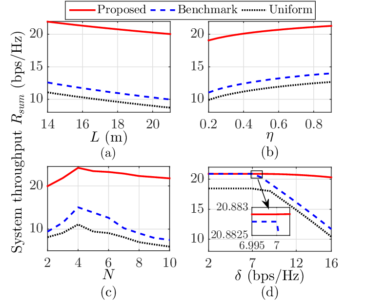
Fig. 4: Impact of system parameters on sum throughput and comparative analysis of different TA schemes.

Further, (18) and (19) can be solved to get,

Φ⁡(Kb​τ0∗)=μ2∗​ln⁡2.\Phi(K_{b}\tau^{*}_{0})=\mu^{*}_{2}\ln{2}. (21)

Now, from (17), (20) and (21),

γ11+γ1​τ0∗τ1∗​Φ⁡(Kb​τ0∗)Φ⁡(γ1​τ0∗τ1∗)+Γb1+Kb​τ0∗=Φ⁡(Kb​τ0∗).\frac{\gamma_{1}}{1+\frac{\gamma_{1}\tau^{*}_{0}}{\tau^{*}_{1}}}\frac{\Phi(K_{b}\tau^{*}_{0})}{\Phi\hskip-1.42262pt\left(\hskip-1.42262pt\frac{\gamma_{1}\tau^{*}_{0}}{\tau^{*}_{1}}\hskip-1.42262pt\right)\hskip-1.42262pt}+\frac{\Gamma_{b}}{1+K_{b}\tau^{*}_{0}}=\Phi(K_{b}\tau^{*}_{0}). (22)

As a result, using (15) and (22), we have

Φ⁡(Kb​τ0∗)​[1−γ12δτ1∗​1Φ⁡(2δτ1∗−1)]=Γb1+Kb​τ0∗.\Phi(K_{b}\tau^{*}_{0})\left[1\hskip-1.42262pt-\hskip-1.42262pt\frac{\gamma_{1}}{2^{\frac{\delta}{\tau^{*}_{1}}}}\frac{1}{\Phi\hskip-1.42262pt\left(2^{\frac{\delta}{\tau^{*}_{1}}}-1\hskip-1.42262pt\right)}\right]=\hskip-1.42262pt\frac{\Gamma_{b}}{1+K_{b}\tau^{*}_{0}}. (23)

Finally, using Kb=Γb1−[τ1∗γ1​(2δτ1∗−1)+τ1∗]K_{b}\hskip-1.42262pt=\hskip-1.42262pt\frac{\Gamma_{b}}{1-\left[\frac{\tau^{*}_{1}}{\gamma_{1}}\left(2^{\frac{\delta}{\tau^{*}_{1}}}-1\right)+\tau^{*}_{1}\right]} obtained from (7), (15), (19), in (23), a univariable eq. in τ1∗\tau^{*}_{1} can be written as:

Φ⁡(g⁡(τ1∗))​[1−γ12δτ1∗​1Φ⁡(2δτ1∗−1)]−Γb1+g⁡(τ1∗)=0,\displaystyle\Phi\Bigl(g\left(\tau^{*}_{1}\right)\Bigr)\left[1\hskip-1.42262pt-\hskip-1.42262pt\frac{\gamma_{1}}{2^{\frac{\delta}{\tau^{*}_{1}}}}\frac{1}{\Phi\hskip-1.42262pt\left(2^{\frac{\delta}{\tau^{*}_{1}}}-1\hskip-1.42262pt\right)}\right]-\frac{\Gamma_{b}}{1+g(\tau^{*}_{1})}=0, (24)

where g⁡(τ1∗)=Γb​[τ1∗​(2δτ1∗−1)]γ1​[1−{τ1∗γ1​(2δτ1∗−1)+τ1∗}]g(\tau^{*}_{1})=\frac{\Gamma_{b}\left[\tau^{*}_{1}\left(2^{\frac{\delta}{\tau^{*}_{1}}}-1\right)\right]}{\gamma_{1}\left[1-\left\{\frac{\tau^{*}_{1}}{\gamma_{1}}\left(2^{\frac{\delta}{\tau^{*}_{1}}}-1\right)+\tau^{*}_{1}\right\}\right]}.

In order to solve (24) in τ1∗=τ1​b\tau^{*}_{1}=\tau_{1b}, we use Golden Section Line Search (GSLS) method [9]. The number of computations NCG​SN_{C}^{GS} in GSLS algorithm is given by NCG​S=⌈2−2.08​ln⁡(ξτ1​bU−τ1​bL)⌉N_{C}^{GS}=\left\lceil 2-2.08\,{\ln\left(\frac{\xi}{\tau_{1b}^{U}-\tau_{1b}^{L}}\right)}\right\rceil, where ξ\xi is the acceptable tolerance, τ1​bL\tau_{1b}^{L} and τ1​bU\tau_{1b}^{U} are respectively the lower and upper bound on τ1​b\tau_{1b}.

IV-C Proposed Algorithm Implementation

Here we propose Algorithm 1 to summarize semi-closed-form for globally optimal TA solution. The case becomes infeasible, when R1≜R1t​hR_{1}\triangleq R^{th}_{1} cannot be met even after allocating all the resources to PU. Thus, R1t​h=τ1t​h​log2⁡(1+γ1​τ0t​hτ1t​h)R^{th}_{1}\hskip-1.42262pt=\hskip-1.42262pt\tau^{th}_{1}\log_{2}\left(1+\frac{\gamma_{1}\tau^{th}_{0}}{\tau^{th}_{1}}\right), where τ0t​h≜f⁡(γ1)−1γ1+f⁡(γ1)−1\tau^{th}_{0}\triangleq\frac{f(\gamma_{1})-1}{\gamma_{1}+f(\gamma_{1})-1} and τ1t​h≜γ1γ1+f⁡(γ1)−1\tau^{th}_{1}\triangleq\frac{\gamma_{1}}{{\gamma_{1}+f(\gamma_{1})-1}} from (13) and (14) respectively, because N=0N=0, Γa=γ1\Gamma_{a}=\gamma_{1} at infeasibility. So, Algorithm 1 starts with a value of δ\delta, and tests the feasibility conditions. It returns the feasible KKT point (τk∗,μ1∗,μ2∗)(\tau^{*}_{k},\mu^{*}_{1},\mu^{*}_{2}), which is the globally-optimal TA solution.

Algorithm 1 Semi-closed-form globally-optimal TA solution
1: δ\delta, R1t​hR^{th}_{1}, τ1​bL\tau^{L}_{1b}, τ1​bU\tau^{U}_{1b} and ζ>0\zeta>0
2: τk∗​∀k∈𝒩0\tau^{*}_{k}\,\forall k\in\mathcal{N}_{0}, μ1∗\mu^{*}_{1}, μ2∗\mu^{*}_{2}
3: if δ>R1t​h{\delta}>R^{th}_{1} then  this case is infeasible
4: else if δ<R1​a{\delta}<R_{1a}, where R1​aR_{1a} is the value of R1R_{1} at τ0=τ0​a\tau_{0}=\tau_{0a} from (13) and τ1=τ1​a\tau_{1}=\tau_{1a} from (14) then
5:      τk∗=τk​a\tau^{*}_{k}=\tau_{ka} using (13) and (14), μ1∗=0\mu^{*}_{1}=0, μ2∗=μ2​a\mu^{*}_{2}=\mu_{2a}
6: else if R1​a≤δ≤R1t​hR_{1a}\leq\delta\leq R^{th}_{1} then
7:      Using GSLS τ1∗=τ1​b\tau^{*}_{1}=\tau_{1b}
8:      τ0∗=τ0​b≜τ1​bγ1​(2δτ1​b−1)\tau^{*}_{0}=\tau_{0b}\triangleq\frac{\tau_{1b}}{\gamma_{1}}\left(2^{\frac{\delta}{\tau_{1b}}}-1\right) by (15), Kb=Γb1−τ0​b−τ1​bK_{b}=\frac{\Gamma_{b}}{1-\tau_{0b}-\tau_{1b}}
9:      τj∗=τj​b≜γjKb\tau^{*}_{j}=\tau_{jb}\triangleq\frac{\gamma_{j}}{K_{b}} ∀j∈{2,3,…​N+1}\forall j\in\{2,3,...N+1\} using (19)
10:      μ2∗=μ2​b≜Φ⁡(Kb​τ0​b)ln⁡2\mu^{*}_{2}=\mu_{2b}\triangleq\frac{\Phi(K_{b}\tau_{0b})}{\ln 2} as obtained using (21)
11:      μ1∗=μ1​b≜μ2​b​ln⁡2Φ⁡(γ1​τ0​bτ1​b)−1\mu^{*}_{1}=\mu_{1b}\triangleq\frac{\mu_{2b}\ln 2}{\Phi\left(\gamma_{1}\frac{\tau_{0b}}{\tau_{1b}}\right)}-1 as obtained using (17)

V Performance Evaluation and Conclusion

In this section, we first numerically validate the proposed optimal TA and then compare it against two existing TA schemes: 1) a near-optimal TA solution [4] as found without considering any δ\delta, and 2) a uniform TA with τk=TN+1,∀k∈𝒩0\tau_{k}=\frac{T}{N+1},\forall k\in\mathcal{N}_{0}. Unless explicitly stated, we have taken L=21L=21 m, N=4N\hskip-1.42262pt=\hskip-1.42262pt4, P0=10P_{0}\hskip-1.42262pt=\hskip-1.42262pt10 W, σ2=−100\sigma^{2}\hskip-1.42262pt=\hskip-1.42262pt-100 dBm, η=0.5\eta=0.5, δ=18\delta\hskip-1.42262pt=\hskip-1.42262pt18 bps/Hz, β=α​d−ζ\beta\hskip-1.42262pt=\hskip-1.42262pt\alpha d\hskip-1.42262pt^{-\zeta}, where α=(3×1084​π​ν)2\alpha\hskip-1.42262pt=\hskip-1.42262pt\left(\frac{3\times 10^{8}}{4\pi\nu}\right)^{2} being the average channel attenuation at unit reference distance with transmitter frequency ν=915\nu\hskip-1.42262pt=\hskip-1.42262pt915 MHz, dd is the distance between two TR pairs, and ζ=3\zeta=3 is the path-loss exponent. Practically, the values of average harvested energies by PU and SU depend upon the underlying channel characteristics.

In Fig. 3, for validating over optimal TA solution, we plot the system throughput against the WPT time for different sets of NN and δ\delta. The optimal TA values as obtained using the proposed algorithm are found to exactly match the maximum Rs​u​mR_{sum} in the feasible region. However, when δ\delta is high, the SUs’ throughput degrades due to lesser TA for SU, resulting in reduced Rs​u​mR_{sum} at optimal τ0∗\tau^{*}_{0}. Further, when NN is large, more number of SUs leads to more harvested energy for PU as well as other SUs, hence the overall throughput increases.

Fig. 4 depicts the impact of system parameters on Rs​u​mR_{sum}, thereby comparing the performance of different TA schemes. In Fig. 4(a), increase in LL increases the distance between two TR pairs, which leads to reduced channel gain. Further, if η\eta is high in Fig. 4(b), more power can be harvested through EH, thereby enhancing Rs​u​mR_{sum}. In Fig. 4(c), Rs​u​mR_{sum} degrades after N=4N=4 which is optimal, as further increase in NN (for a fixed LL) curtails the TA for WPT as well as WIT. In Fig. 4(d), benchmark approaches proposed scheme for lower values of δ\delta, but still lagging behind as it doesn’t consider all the EH possibilities. However, for large δ\delta, system performance drastically improves for proposed scheme. Similarly with respect to LL, η\eta as well as NN, the proposed scheme performs significantly better than other two. This is because, unlike in proposed scheme, the effect of a minimum PU throughput is not taken into consideration in other TA schemes, and hence the throughput cannot be maximized for higher δ\delta corresponding to QoS-aware applications. In nutshell, on an average against all the parameters, proposed scheme is found to outperform benchmark scheme by 70%70\% and uniform fixed TA scheme by 101%101\%.

So, to summarize, we proposed a novel WPT framework in a CR scenario, by exploiting all possible RF-EH opportunities. We obtained semi-closed-form for globally optimal TA solution by maximizing the system throughput. The results are numerically validated, and remarkable performance enhancement is achieved over benchmark and uniform TA schemes.

References

  • [1] J. Yan and Y. Liu, “A dynamic SWIPT approach for cooperative cognitive radio networks,” IEEE Trans. Veh. Technol., vol. 66, no. 12, pp. 11 122–11 136, Dec. 2017.
  • [2] S. Yin, E. Zhang, Z. Qu, L. Yin, and S. Li, “Optimal cooperation strategy in cognitive radio systems with energy harvesting,” IEEE Trans. Wireless Commun., vol. 13, no. 9, pp. 4693–4707, Sept. 2014.
  • [3] M. Zheng, C. Xu, W. Liang, and H. Yu, “Harvesting-throughput tradeoff for RF-powered underlay cognitive radio networks,” Electron. Lett., vol. 52, no. 10, pp. 881–883, 2016.
  • [4] D. Xu and Q. Li, “Joint power control and time allocation for wireless powered underlay cognitive radio networks,” IEEE Wireless Commun. Lett., vol. 6, no. 3, pp. 294–297, June 2017.
  • [5] A. P. Shrestha and S. Yoo, “Optimal resource allocation using support vector machine for wireless power transfer in cognitive radio networks,” IEEE Trans. Veh. Technol., vol. 67, no. 9, pp. 8525–8535, Sept. 2018.
  • [6] A. El Shafie, N. Al-Dhahir, and R. Hamila, “Cooperative access schemes for efficient SWIPT transmissions in cognitive radio networks,” in Proc. IEEE Globecom Workshops (GC Wkshps), Dec. 2015, pp. 1–6.
  • [7] S. Boyd and L. Vandenberghe, Convex optimization. Cambridge University Press, 2004.
  • [8] E. W. Weisstein, “Lambert W-function,” 2002. [Online]. Available: http://mathworld.wolfram.com/LambertW-Function.html
  • [9] A. D. Belegundu and T. R. Chandrupatla, Optimization concepts and applications in engineering. Cambridge University Press, 2019.
  • [10] X. Lu, I. Flint, D. Niyato, N. Privault, and P. Wang, “Self-sustainable communications with RF energy harvesting: Ginibre point process modeling and analysis,” IEEE J. Sel. Areas in Commun., vol. 34, no. 5, pp. 1518–1535, May 2016.