Trace of anomalous diffusion in a biased quenched trap model

Takuma Akimoto Email: takuma@rs.tus.ac.jp Affiliation: Department of Physics, Tokyo University of Science, Noda, Chiba 278-8510, Japan Keiji Saito Affiliation: Department of Physics, Keio University, Yokohama, 223-8522, Japan

August 11, 2026

Abstract

Diffusion on a quenched heterogeneous environment in the presence of bias is considered analytically. The first-passage-time statistics can be applied to obtain the drift and the diffusion coefficient in periodic quenched environments. We show several transition points at which sample-to-sample fluctuations of the drift or the diffusion coefficient remain large even when the system size becomes large, i.e., non-self-averaging. Moreover, we find that the disorder average of the diffusion coefficient diverges or becomes zero when the corresponding annealed model generates superdiffusion or subdiffusion, respectively. This result implies that anomalous diffusion in an annealed model is traced by anomaly of the diffusion coefficients in the corresponding quenched model.

I Introduction

Anomalous transport characterized by a nonlinear growth of the mean squared displacement (MSD) or the mean displacement (MD) in the presence of bias is a ubiquitous phenomenon in nature. Since a discovery of anomalous transport in amorphous materials Scher and Montroll 1975, considerable efforts have been made to unveil anomalous physical features in experiments such as biological systems Caspi et al. 2000; Wong et al. 2004; Golding and Cox 2006; Szymanski and Weiss 2009; Bronstein et al. 2009; Gal and Weihs 2010; Weigel et al. 2011; Jeon et al. 2011; Tabei et al. 2013; Höfling and Franosch 2013; Manzo et al. 2015. One of physical mechanisms that produce anomalous transport is attributed to a heterogeneous environment, where local diffusivity is spatially heterogeneous or changes with time.

A typical model of anomalous diffusion on heterogeneous environments is a quenched trap model (QTM) Bouchaud and Georges 1990. In this model, the spatial heterogeneity is represented by a quenched random energy landscape. While this model is simple and has been investigated for decades, there are few exact results on the QTM Derrida 1983. This is because one has to take into account how a random walker visits a site. In particular, one needs to calculate the number of visits to a site by a random walker to obtain an exact result. The MSD of the QTM shows anomalous diffusion when the temperature is below the glass temperature, where the mean waiting time diverges Bouchaud and Georges 1990. By a scaling argument, it is known that the power-law exponent of the MSD depends on the spatial dimension Bouchaud and Georges 1990. Furthermore, fluctuations of the diffusion coefficients obtained by single trajectories depend intrinsically on the dimension Miyaguchi and Akimoto 2011; Miyaguchi and Akimoto 2015.

Continuous-time random walk (CTRW) is an annealed model of the QTM, which is widely used to investigate anomalous diffusion because its analytical treatment is possible due to the spatial homogeneity Metzler and Klafter 2000. In the CTRW, the waiting-time distribution does not depend on the site but is identical for all the sites. This is a significant difference between the QTM and the CTRW, which gives a rich physical feature such as sample-to-sample fluctuations Miyaguchi and Akimoto 2011; Miyaguchi and Akimoto 2015; Luo and Tang 2015; Akimoto et al. 2016; *Akimoto2018. However, the CTRW becomes a good approximation of the QTM when the spatial dimension is greater than two or in the presence of bias Machta 1985. In these situations, a random walker can visit a new site at constant non-zero probability, which reduces a risk of returning to the sites that a random walker visited before. Remarkable features of the CTRW are observed in the time-averaged-base MSD (TAMSD). When the mean waiting time diverges, the TAMSD is not coincided with the ensemble-averaged-base MSD, i.e., ergodicity breaking He et al. 2008; Neusius et al. 2009; Miyaguchi and Akimoto 2013; Metzler et al. 2014. In our previous studies Akimoto et al. 2016; *Akimoto2018, we showed that the QTM with finite system size is ergodic; i.e., the TAMSD is equivalent to the corresponding MSD, and that the TAMSD becomes non-self-averaging when the temperature is below the glass temperature.

Effects of bias in the CTRW have been investigated in the regime where the mean waiting time is finite but the second moment diverges. In this regime, the drift is normal but the variance of the displacement (VD) shows superdiffusion, whereas the MSD in the absence of bias is normal Burioni et al. 2013; *Burioni2014; Akimoto et al. 2018b; *hou2018biased. This phenomenon is called field-induced superdiffusion. Field-induced superdiffusion is ubiquitous phenomenon observed in crowded systems such as supercooled liquids Schroer and Heuer 2013; Bénichou et al. 2013; Bénichou et al.; Gradenigo et al. 2016; Leitmann and Franosch 2017. However, field-induced superdiffusion in heterogeneous quenched environments has not been studied so far.

In this paper, we discuss how a bias affects transport properties in the QTM with a finite system size, where we assume a periodic boundary condition. In a periodic system, the first-passage-time (FPT) statistics plays an important role in obtaining the transport properties such as drift and diffusivity Reimann et al. 2001; *Reimann2002. Applying the FPT statistics in a biased QTM Akimoto and Saito 2019, we show non-self-averaging properties of the MD and the VD. Comparing with the CTRW results, we provide an interesting connection between the annealed and quenched models.

II model

Here, we consider a random walk on a one-dimensional random energy landscape, i.e., QTM Bouchaud and Georges 1990, where the energy landscape is quenched, and assume that the landscape is arranged periodically. The probabilities of stepping to the right and the left site are denoted by $p$ and $q=1-p$ , respectively. We assume that the lattice constant is unity and that the tops of the potentials are flat; i.e., the tops are the same hight for all sites. In other words, probabilities $p$ and $q$ do not depend on the site. In particular, we consider the case of $p\neq\frac{1}{2}$ , i.e., a biased QTM, and $p>1/2$ for simplicity.

Quenched disorder implies that when realizing the random energy landscape it does not change with time. The number of lattice sites with different energies is $L$ ; i.e., the energy landscape of the system is periodically arranged with period $L$ . At each lattice point, the depth $E>0$ of an energy trap is randomly assigned and quenched. The depths are independent identically distributed random (IID) variables with an exponential distribution, $\rho(E)=T^{-1}_{g}\exp(-E/T_{g})$ , where $T_{g}$ is called a glass temperature. A particle can escape from a trap and jump to one of the nearest neighbors. Escape times from a trap are IID random variables with an exponential distribution and follows the Arrhenius law; i.e., the mean escape time of the $k$ th site is given by $\tau_{k}=\tau_{c}\exp(E_{k}/T)$ , where $E_{k}$ is the depth of the energy at site $k$ , $T$ the temperature, and $\tau_{c}$ a typical time. The probability that escape time $\tau$ is smaller than $x$ is given by $\Pr(\tau\leq x)\cong\Pr(E\leq T\ln(x/\tau_{c}))$ . Because the probability density function (PDF) of random variable $E$ follows $\rho(E)$ , the PDF of $\tau$ for infinite systems, denoted by $\psi_{\alpha}(\tau)$ , becomes

\int_{\tau}^{\infty}d\tau^{\prime}\psi_{\alpha}(\tau^{\prime})\cong\left(\frac{\tau}{\tau_{c}}\right)^{-\alpha}\quad(\tau\geq\tau_{c})

(1)

with $\alpha\equiv T/T_{g}$ Bardou et al. 2002; Akimoto et al. 2018a.

The master equation of the biased QTM can be represented by the quenched disorder realization. Let $P_{k}(t)$ be the probability of finding a particle at site ${k}$ at time $t$ . The master equation for the $i$ th disorder realization, where the mean escape time at site $k$ is denoted by $\tau_{k}^{(i)}$ , is given by

\frac{dP_{k}(t)}{dt}=p\frac{P_{k-1}(t)}{\tau_{k-1}^{(i)}}+q\frac{P_{k+1}(t)}{\tau_{k+1}^{(i)}}-\frac{P_{k}(t)}{\tau_{k}^{(i)}}.

(2)

We consider the periodic boundary condition, i.e., $P_{0}(t)=P_{L}(t)$ , $P_{L+1}(t)=P_{1}(t)$ , $\tau_{0}^{(i)}=\tau_{L}^{(i)}$ , and $\tau_{L+1}^{(i)}=\tau_{1}^{(i)}$ . It follows that the steady state can be obtained as

P_{k}^{\rm st}=\frac{\tau_{k}^{(i)}}{L\mu_{i}},

(3)

where $P_{k}^{\rm st}$ is the probability of finding a particle at site $k$ in the steady state and $\mu_{i}$ is the sample mean for the $i$ th disorder realization:

\mu_{i}=\frac{1}{L}\sum_{k=0}^{L-1}\tau_{k}^{(i)}.

(4)

The steady state is exactly the same as the equilibrium state under no bias Akimoto et al. 2016; Akimoto et al. 2018a. This is because the bias we consider here does not change the shape of the random energy landscape.

III First-passage-time statistics and diffusive properties

In our previous study Akimoto and Saito 2019, we derive the first-passage-time (FPT) statistics for the biased QTM. Here, we review the FPT statistics in the biased QTM and show that they play an important role in obtaining the diffusive properties such as drift and diffusivity in the system. The FPT in the biased QTM is defined as the time when a particle starting from the origin reaches site $L$ , i.e., the right boundary. We note that the target is located at site $L$ only (site $-L$ is not a target) whereas we consider a periodic landscape. In the large- $L$ limit, the mean FPT (MFPT) and the variance of the FPT (VFPT) for the $i$ th disorder realization are represented by

	$\displaystyle\langle T\rangle$	$\displaystyle\sim\frac{L\mu_{i}}{p-q},$		(5)
	$\displaystyle\langle\delta T^{2}\rangle$	$\displaystyle\sim\frac{L\{\sigma_{i}^{2}(p-q)+\mu_{i}^{2}\}}{(p-q)^{3}},$		(6)

where $\delta T\equiv T-\langle T\rangle$ and $\sigma_{i}^{2}$ is the sample variance, i.e.,

\sigma_{i}^{2}=\frac{1}{L}\sum_{n=0}^{L-1}(\tau_{n}^{(i)})^{2}-\mu_{i}^{2}\,.

(7)

These formulae are exact for any quenched disorder realizations in the large- $L$ limit and depend crucially on the disorder realization. Therefore, sample-to-sample fluctuations for the MFPT and the VFPT become significant when $\alpha$ is smaller than two Akimoto and Saito 2019.

Here, we connect the FPT statistics with the MD and the VD. Let $n_{t}$ be the number of events that a particle crosses the right boundary, i.e., stepping from $L-1$ to $L$ site, which is equivalent to make a counterclockwise revolution on a ring. In the large- $L$ limit, the probability that a particle starting from the origin crosses the left boundary, i.e., stepping from $-L+1$ to $-L$ site, becomes zero. Therefore, a particle always resides in a interval $[(n_{t}-1)L,n_{t}L)$ in the large- $L$ limit. It follows that the displacement, $\delta x_{t}\equiv x(t)-x(0)$ , can be represented by

\delta x_{t}=Ln_{t}+C_{L},

(8)

where $x(t)$ is a position of a particle at time $t$ and $C_{L}$ is a residual term that is considered to be a random variable whose support is $-L<C_{L}<L$ , and thus $\langle|C_{L}|\rangle=O(L)$ . Because time when a particle crosses the right boundary is an IID random variable, the process of $n_{t}$ is described by a renewal process Cox 1962. By the renewal theory Cox 1962, the mean of $n_{t}$ is given by

\langle n_{t}\rangle\sim\frac{t}{\mu}\quad(t\to\infty),

(9)

where $\mu$ is the mean inter-event time, which is equivalent to MFPT $\langle T\rangle$ . Therefore, the MD is represented by

\langle\delta x_{t}\rangle\sim\frac{L}{\langle T\rangle}t.

(10)

This formula is applicable for any diffusion processes when the landscape is periodic Reimann et al. 2001; *Reimann2002. Applying the MFPT of the biased QTM, i.e., Eq. (5), we have

\langle\delta x_{t}\rangle\sim L\langle n_{t}\rangle\sim\frac{\varepsilon}{\mu_{i}}t\quad(t\to\infty),

(11)

where $\varepsilon=p-q$ .

Using Eq. (8), we have

\delta x_{t}^{2}=L^{2}n_{t}^{2}+2LC_{L}n_{t}+C_{L}^{2}.

(12)

It follows that the variance of $\delta x_{t}$ is given by

\langle\delta x_{t}^{2}\rangle-\langle\delta x_{t}\rangle^{2}\sim L^{2}(\langle n_{t}^{2}\rangle-\langle n_{t}\rangle^{2})\quad(t\to\infty),

(13)

where we used a fact that $C_{L}$ and $n_{t}$ are independent, i.e., $\langle C_{L}n_{t}\rangle=\langle C_{L}\rangle\langle n_{t}\rangle$ . By the renewal theory Cox 1962, the variance of $n_{t}$ is derived for $t\gg 1$ as

\langle n_{t}^{2}\rangle-\langle n_{t}\rangle^{2}\sim\frac{\langle T^{2}\rangle-\langle T\rangle^{2}}{\langle T\rangle^{3}}t,

(14)

where $\langle T^{2}\rangle$ is the second moment of the FPT. Therefore, the variance of $\delta x_{t}$ can be represented by

\langle\delta x_{t}^{2}\rangle-\langle\delta x_{t}\rangle^{2}\sim\left(\frac{\varepsilon\sigma_{i}^{2}}{\mu_{i}^{3}}+\frac{1}{\mu_{i}}\right)t

(15)

for $t\to\infty$ . Figure 2 shows a good agreement in between numerical simulations and the theory.

Refer to caption — Figure 1: Mean displacement (MD) for different $\alpha$ (a) $\alpha=0.5$ , (b) $\alpha=1.5$ , and (c) $\alpha=2.5$ ( $p=0.8$ and $\tau_{c}=1$ ). Symbols are the results of MDs for five different disorder realizations ( $L=10^{3}$ ). We note that the average is taken only for the thermal average. Thus, sample-to-sample fluctuations are significant for (a). Solid lines are the disorder averages of the MD, i.e., $\langle\lambda\rangle_{\rm dis}t$ , where $\langle\lambda\rangle_{\rm dis}$ can be calculated by Eq. (26) for $\alpha\leq 1$ and $\langle\lambda\rangle_{\rm dis}=\varepsilon/\langle\mu\rangle_{\rm dis}$ for $\alpha>1$ , which can be calculated by Eq. (1).

IV Self-averaging properties for drift and diffusivity

IV.1 Drift

The asymptotic behavior of the MD is given by Eq. (11). The result becomes exact for any $t>0$ when the initial condition is the steady state of the system, i.e., Eq. (3), because the MD can be described as

\langle\delta x_{t}\rangle_{\rm st}=\varepsilon\langle N_{t}\rangle_{\rm st}

(16)

for any $t>0$ , where $N_{t}$ is the mean number of steps of a particle until time $t$ and $\langle\cdot\rangle_{\rm st}$ is the average when the initial condition is the steady state. When the initial condition is the steady state, $\langle N_{t}\rangle_{\rm st}$ increases linearly with time:

\langle N_{t}\rangle_{\rm st}=\frac{t}{\mu_{i}}

(17)

for any $t>0$ . Hence, the drift defined as $\lambda\equiv\langle\delta x_{t}\rangle_{\rm st}/t$ is given by

\lambda_{i}(L)=\frac{\varepsilon}{\mu_{i}}

(18)

for some disorder realization.

Now, we consider sample-to-sample fluctuations of the drift. When the mean trapping time, $\langle\tau\rangle\equiv\int_{0}^{\infty}\tau\psi_{\alpha}(\tau)d\tau$ , is finite ( $\alpha>1$ ), we have $\mu_{i}\rightarrow\langle\tau\rangle$ ( $L\to\infty$ ) by the law of large numbers. Therefore, in the large- $L$ limit, the drift does not depend on the disorder realization (see Fig. 1). Hence, the drift is self-averaging (SA) for $\alpha>1$ Bouchaud and Georges 1990. To quantify the SA property of $\lambda_{i}$ , we consider the SA parameter defined as Akimoto et al. 2016; Akimoto et al. 2018a

{\rm SA}(L;\lambda)\equiv\frac{\langle\lambda_{i}(L)^{2}\rangle_{\rm dis}-\langle\lambda_{i}(L)\rangle_{\rm dis}^{2}}{\langle\lambda_{i}(L)\rangle_{\rm dis}^{2}},

(19)

where $\langle\cdot\rangle_{\rm dis}$ means the disorder average, i.e., the average obtained under different disorder realizations. The SA parameter becomes zero in the large- $L$ limit when the drift is SA. Using Eq. (18), we have

{\rm SA}(L;\lambda)=\frac{\langle 1/\mu_{i}^{2}\rangle_{\rm dis}-\langle 1/\mu_{i}\rangle_{\rm dis}^{2}}{\langle 1/\mu_{i}\rangle_{\rm dis}^{2}},

(20)

which is the same as the SA parameter for the diffusion coefficient in the absence of bias Akimoto et al. 2016; Akimoto et al. 2018a. For $\alpha>2$ , the SA parameter decays as $L^{-1}$ by the central limit theorem. For $1<\alpha<2$ , it goes to zero as $L\to\infty$ by the law large numbers. However, as shown in Appendix. A, it decays non-trivially as $L^{-\alpha+1}$ in the large- $L$ limit. Therefore, sample-to-sample fluctuations remain large even for a relatively large $L$ when $\alpha$ closes to one.

When the mean trapping time diverges ( $\alpha\leq 1$ ), the law of large numbers does not hold. However, the generalized central limit theorem is still valid, which states that the PDF of the normalized sum of $\tau_{n}^{(i)}$ follows the one-sided Lévy distribution Feller 1971:

\dfrac{\sum_{n=1}^{L}\tau_{n}^{(i)}}{L^{1/\alpha}}\Rightarrow X_{\alpha}\quad(L\to\infty),

(21)

where $X_{\alpha}$ is a random variable following the one-sided Lévy distribution of index $\alpha$ . Therefore, there are large sample-to-sample fluctuations in sample mean $\mu_{i}$ . The PDF of $X_{\alpha}$ , denoted by $l_{\alpha}(x)$ with $x>0$ , can be expressed as an infinite series Feller 1971

l_{\alpha}(x)=-\frac{1}{\pi x}\sum_{k=1}^{\infty}\frac{\Gamma(k\alpha+1)}{k!}(-cx^{-\alpha})^{k}\sin(k\pi\alpha),

(22)

where $c$ is a scale parameter, given by $c=\Gamma(1-\alpha)\tau_{c}^{\alpha}$ for $\psi_{\alpha}(\tau)$ . Here, we define the inverse Lévy distribution as the PDF of $X_{\alpha}^{-1}$ :

g_{\alpha}(y)=-\frac{1}{\pi y}\sum_{k=1}^{\infty}\frac{\Gamma(k\alpha+1)}{k!}(-cy^{\alpha})^{k}\sin(k\pi\alpha),

(23)

where the first and the second moments of $X^{-1}_{\alpha}$ are given by Akimoto et al. 2016

\langle X_{\alpha}^{-1}\rangle=\frac{\Gamma(\frac{1}{\alpha})}{\alpha c^{\frac{1}{\alpha}}},\quad\langle X_{\alpha}^{-2}\rangle=\frac{\Gamma(\frac{2}{\alpha})}{\alpha c^{\frac{2}{\alpha}}}.

(24)

Drift can be represented by

\lambda_{i}(L)=\varepsilon\frac{L}{L^{1/\alpha}}\frac{L^{1/\alpha}}{\tau_{1}+\cdots+\tau_{L}}\sim\varepsilon L^{1-1/\alpha}X_{\alpha}^{-1}

(25)

for $L\to\infty$ . Thus, the PDF of $\lambda_{i}$ is described by the inverse Lévy distribution. Therefore, $\lambda_{i}$ depends crucially on the sample of the disorder realization. Using the first moment of the inverse Lévy distribution Akimoto et al. 2016; Akimoto et al. 2018a, we obtain the exact asymptotic behavior of the disorder average of the drift:

\langle\lambda(L)\rangle_{\rm dis}\sim\frac{\varepsilon L^{1-1/\alpha}\Gamma(\alpha^{-1})}{\alpha\tau_{c}\Gamma(1-\alpha)^{1/\alpha}}.

(26)

Using the first and the second moment of $1/\mu_{i}$ , we have the SA parameter for drift

\lim_{L\to\infty}{\rm SA}(L;\lambda)=\left\{\begin{array}[]{ll}0&(\alpha>1)\\ \\ \dfrac{\alpha\Gamma(\frac{2}{\alpha})}{\Gamma(\frac{1}{\alpha})^{2}}-1&(\alpha\leq 1).\end{array}\right.

(27)

For $\alpha<1$ , the SA parameter is a non-zero constant, and thus $\lambda_{i}$ becomes non-SA; i.e., there are large sample-to-sample fluctuations in the drift [see Fig. 1(a)]. Therefore, the transition temperature from SA to non-SA behavior in the drift is given by $T_{c}=T_{g}$ .

IV.2 Diffusivity

Here, we consider the VD to characterize the diffusivity of the system, which is defined as

{\rm Var}(\delta{x}_{t})_{\rm st}\equiv\langle\delta{x}_{t}^{2}\rangle_{\rm st}-\langle\delta{x}_{t}\rangle_{\rm st}^{2}.

(28)

By Eq. (15), the asymptotic behavior of the VD increases linearly with time:

{\rm Var}(\delta{x}_{t})_{\rm st}\sim\left(\frac{\varepsilon\sigma_{i}^{2}}{\mu_{i}^{3}}+\frac{1}{\mu_{i}}\right)t

(29)

for $t\gg 1$ and $L\gg 1$ . Therefore, the diffusion coefficient of the system, i.e., $D_{i}(L)\equiv\displaystyle\lim_{t\to\infty}{\rm Var}(\delta{x}_{t})_{\rm st}/(2t)$ , is given by

D_{i}(L)\sim\frac{1}{2}\left(\frac{\varepsilon\sigma_{i}^{2}}{\mu_{i}^{3}}+\frac{1}{\mu_{i}}\right)

(30)

for $L\to\infty$ . The disorder average of $D_{i}(L)$ is given by

\langle D(L)\rangle_{\rm dis}\sim\frac{1}{2}\left(\varepsilon\left\langle\frac{\sigma_{i}^{2}}{\mu_{i}^{3}}\right\rangle_{\rm dis}+\left\langle\frac{1}{\mu_{i}}\right\rangle_{\rm dis}\right)

(31)

for $L\to\infty$ . For $\alpha>2$ , the second moment of trapping times exists; i.e., $\langle\tau^{2}\rangle\equiv\int_{0}^{\infty}\tau^{2}\psi(\tau)d\tau<\infty$ . It follows that the disorder average of $D_{i}(L)$ is finite and given by

\langle D(L)\rangle_{\rm dis}\sim\frac{1}{2}\left(\varepsilon\frac{\langle\tau^{2}\rangle-\langle\tau\rangle^{2}}{\langle\tau\rangle^{3}}+\frac{1}{\langle\tau\rangle}\right)

(32)

for $L\to\infty$ and $\alpha>2$ .

For $\alpha<2$ , the disorder average of $\{\tau_{n}^{(i)}\}^{2}$ diverges. To compute the disorder average of $\sigma_{i}^{2}/\mu_{i}^{3}$ , we consider the scaling of the sum of $\{\tau_{n}^{(i)}\}^{2}$ . The PDF of $\{\tau_{n}^{(i)}\}^{2}$ is given by

\psi_{2,\alpha}(x)=\frac{1}{2\sqrt{x}}\psi_{\alpha}(\sqrt{x}),

(33)

because $\Pr(\tau^{2}\leq x)=\Pr(\tau\leq\sqrt{x})=\int_{0}^{\sqrt{x}}\psi_{\alpha}(x^{\prime})dx^{\prime}$ . For $x\to\infty$ , the PDF becomes

\psi_{2,\alpha}(x)\propto x^{-1-\alpha/2}\propto\psi_{\alpha/2}(x).

(34)

By the generalized central limit theorem Feller 1971, normalized sum $X_{\frac{\alpha}{2}}(L)$ , defined by

X_{\frac{\alpha}{2}}(L)\equiv\frac{1}{L^{2/\alpha}}\sum_{n=1}^{L}\{\tau_{n}^{(i)}\}^{2},

(35)

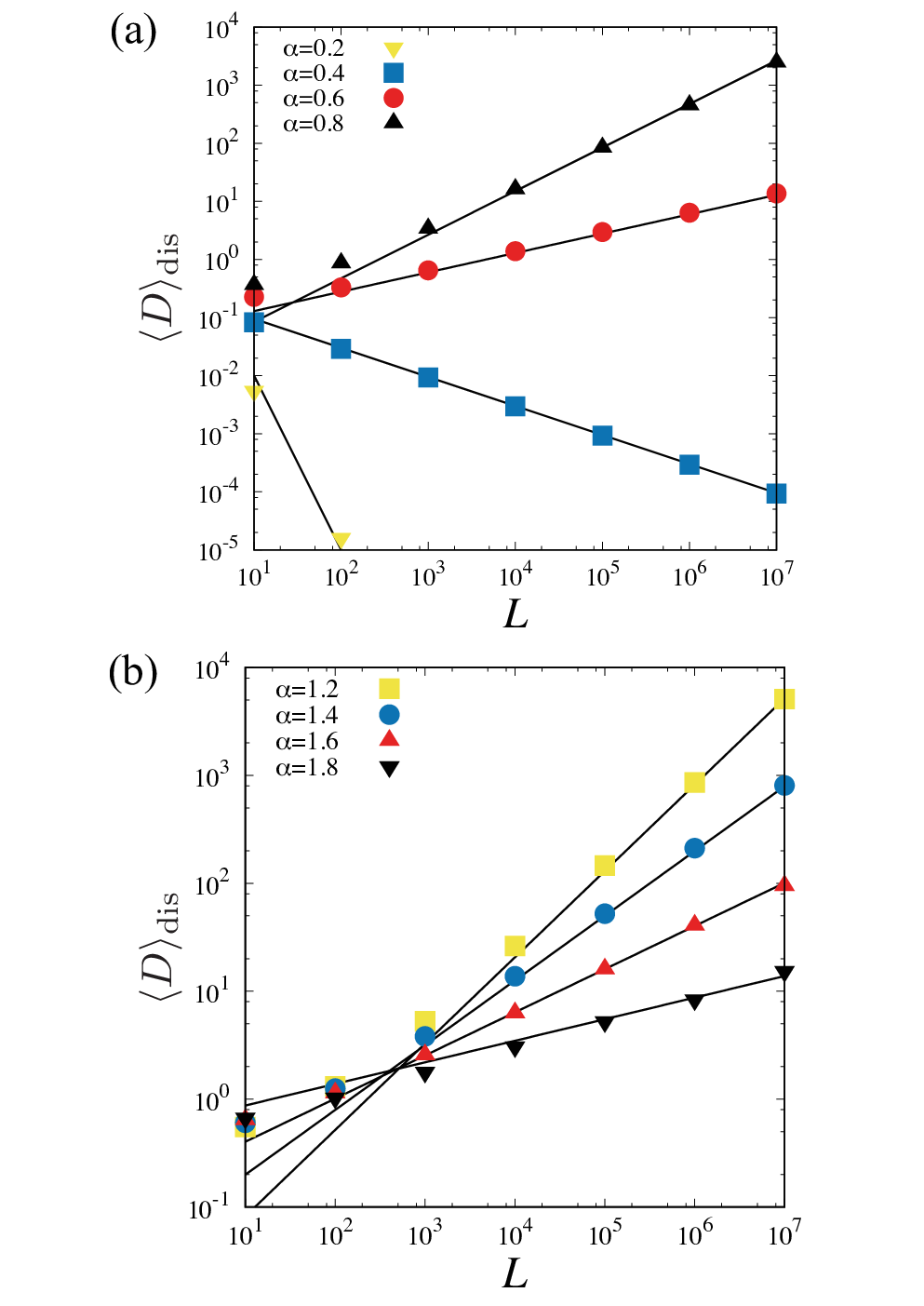
converges in distribution to a random variable with the one-sided Lévy distribution of index $\alpha/2$ . For $1<\alpha<2$ , $\langle\tau\rangle$ is finite but $\langle\tau^{2}\rangle$ diverges. Therefore, $D_{i}(L)$ is proportional to $\sigma_{i}^{2}/\mu^{3}_{i}$ , which depends on $L$ . As shown in Appendix B, the disorder average of $D_{i}(L)$ increases with $L$ :

\langle D(L)\rangle_{\rm dis}\propto L^{2-\alpha}

(36)

for $L\to\infty$ , which means that the diffusion coefficient diverges in the large- $L$ limit [see Fig. 3(b)]. This divergence of the diffusion coefficient is a manifestation of field-induced superdiffusion in the corresponding annealed system, i.e., the biased CTRW Burioni et al. 2014. This is because the variance of the displacement exhibits superdiffusion, i.e., ${\rm Var}(\delta{x}_{t})_{\rm st}\propto t^{3-\alpha}$ , which means that a standard diffusion coefficient diverges.

For $\alpha<1$ , both the first and the second moments of the trapping times diverge. The scalings of the sums of $\tau_{n}^{(i)}$ and $\{\tau_{n}^{(i)}\}^{2}$ follows

\sum_{n=1}^{L}\tau_{n}=O(L^{1/\alpha})\quad{\rm and}\quad\sum_{n=1}^{L}\{\tau_{n}^{(i)}\}^{2}=O(L^{2/\alpha})

(37)

for $L\to\infty$ . Since $D_{i}(L)$ is proportional to $\sigma_{i}^{2}/\mu^{3}_{i}$ , we have

D_{i}(L)\propto\frac{\sigma_{i}^{2}}{\mu^{3}_{i}}\propto L^{2}\frac{\sum_{n=1}^{L}\tau_{n}^{2}}{(\sum_{n=1}^{L}\tau_{n})^{3}}\propto L^{2-1/\alpha}.

(38)

It follows that the scaling of the disorder average of $D_{i}(L)$ becomes

\langle D(L)\rangle_{\rm dis}\propto L^{2-1/\alpha}

(39)

Hence, the diffusion coefficient diverges for $\alpha>1/2$ , whereas it becomes zero for $\alpha<1/2$ [see Fig. 3(a)]. This is physically reasonable because the variance of the displacement in the CTRW with drift becomes superdiffusive and subdiffusive for $\alpha>1/2$ and $\alpha<1/2$ , respectively.

Let us consider the SA property for the diffusion coefficient. The SA parameter is defined as

{\rm SA}(L;D)\equiv\frac{\langle D(L)^{2}\rangle_{\rm dis}-\langle D(L)\rangle_{\rm dis}^{2}}{\langle D(L)\rangle_{\rm dis}^{2}}.

(40)

The SA parameter goes to zero in the large- $L$ limit when the diffusion coefficient is SA.

For $\alpha>2$ , the second moment of trapping times exists; i.e., $\langle\tau^{2}\rangle\equiv\int_{0}^{\infty}\tau^{2}\psi(\tau)d\tau<\infty$ . Therefore, sample variance $\sigma_{i}^{2}$ converges to $\langle\tau^{2}\rangle-\langle\tau\rangle^{2}$ as $L\to\infty$ . Hence, the sample mean and the sample mean of the squared trapping times are converges to constants, which means $\langle D(L)^{2}\rangle_{\rm dis}-\langle D(L)\rangle_{\rm dis}^{2}\to 0$ for $L\to\infty$ . Therefore, the diffusion coefficient is SA for $\alpha>2$ .

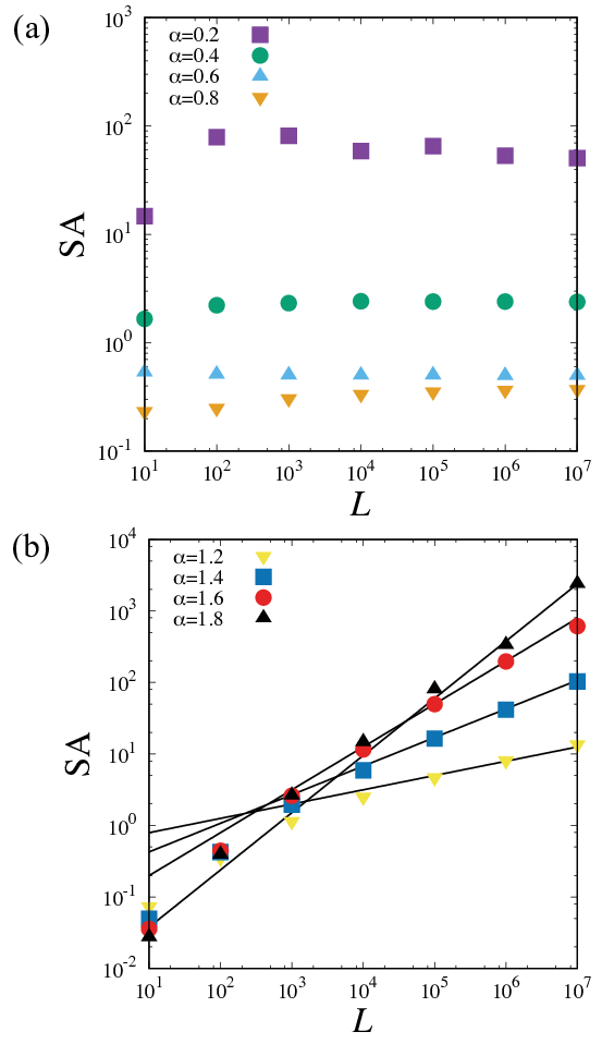
For $1<\alpha<2$ , the second moment of $D_{i}(L)$ is also calculated in Appendix. B. As shown in Fig. 4(b), the SA parameter increases with $L$ . In particular, it diverges as

{\rm SA}(L;D)\propto\frac{\langle D(L)^{2}\rangle_{\rm dis}}{\langle D(L)\rangle_{\rm dis}^{2}}\propto L^{\alpha-1}

(41)

for $L\to\infty$ . It follows that the diffusion coefficient is non-SA for $1<\alpha<2$ .

For $\alpha<1$ , both the first and the second moment of the trapping times diverge. By Eq. (38) and $\sum_{n=1}^{L}\tau_{n}^{2}<\left(\sum_{n=1}^{L}\tau_{n}\right)^{3}$ , $D_{i}(L)$ can be represented as

D_{i}(L)\sim\frac{\varepsilon L^{2-1/\alpha}}{2}C_{i}(L),

(42)

where $C_{i}(L)=L^{1/\alpha}\sum_{n=1}^{L}\tau_{n}^{2}/\left(\sum_{n=1}^{L}\tau_{n}\right)^{3}$ is a random variable depending on the disorder realization. Therefore, the SA parameter becomes

{\rm SA}(L;D)=\frac{\langle D(L)^{2}\rangle_{\rm dis}}{\langle D(L)\rangle_{\rm dis}^{2}}-1=\frac{\langle C(L)^{2}\rangle_{\rm dis}}{\langle C(L)\rangle_{\rm dis}^{2}}-1,

(43)

which is a finite value because $1/\left(\sum_{n=1}^{L}\tau_{n}\right)^{3}<C_{i}(L)<1$ , i.e., $0<\langle C_{i}(L)\rangle_{\rm dis}<1$ and $0<\langle C_{i}(L)^{2}\rangle_{\rm dis}<1$ . Thus, ${\rm SA}(L;D)\to S(\alpha)>0$ for $L\to\infty$ ; i.e., the diffusion coefficient is non-SA for $\alpha<1$ [see Fig. 4(a)].

V Conclusion

The MD and the VD are always normal in a biased QTM with a finite system size with the aid of a stationary steady state, which is different from the biased CTRW. Using the FPT statistics, we have provided exact results for the drift and the diffusion coefficient in the biased QTM. We have found that anomaly of the disorder average of the diffusion coefficient is a manifestation of anomalous diffusion in the corresponding annealed model (CTRW). In particular, divergence and zero of the disorder average of the diffusion coefficient, i.e., $\langle D\rangle_{\rm dis}$ , in the biased QTM implies superdiffusion and subdiffusion in the biased CTRW, respectively (see Fig. 5). Moreover, we have introduced the SA parameter to quantify the SA property. Transition points between SA and non-SA are $\alpha=1$ and $\alpha=2$ for the MD and the VD, respectively.

Acknowledgement

T.A. was supported by JSPS Grant-in-Aid for Scientific Research (No. C JP18K03468) and K.S. was supported by JSPS Grants-inAid for Scientific Research (JP17K05587).

Appendix A Scaling of the SA parameter for drift

Here, we show a power-law decay of the SA parameter for drift. For $1<\alpha<2$ , it decays as $L^{1-\alpha}$ , where $L$ is the system size. Drift for a sample realization is given by

\lambda(L)=\frac{\varepsilon L}{\tau_{1}+\cdots+\tau_{L}}=\frac{\varepsilon L}{L^{1/\alpha}\tilde{X}_{\alpha}(L)+\langle\tau\rangle L},

(44)

where

\tilde{X}_{\alpha}(L)=\frac{\tau_{1}+\cdots+\tau_{L}-\langle\tau\rangle L}{L^{1/\alpha}}.

(45)

In the large- $L$ limit, the PDF of $\tilde{X}_{\alpha}(L)$ converges to the Lévy distribution of index $\alpha$ . For $L^{1/\alpha-1}\tilde{X}_{\alpha}(L)\ll\langle\tau\rangle\varepsilon$ , $\lambda(L)$ becomes

\lambda(L)\cong\frac{\varepsilon}{\langle\tau\rangle}-\frac{\varepsilon L^{1/\alpha-1}\tilde{X}_{\alpha}(L)}{\langle\tau\rangle^{2}}.

(46)

On the other hand, it becomes

\lambda(L)\cong\frac{\varepsilon L^{1-1/\alpha}}{\tilde{X}_{\alpha}(L)}

(47)

for $L^{1/\alpha-1}\tilde{X}_{\alpha}(L)\gg\langle\tau\rangle\varepsilon$ . The ensemble average of $\tilde{X}_{\alpha}(L)^{2}$ restricted in $\tilde{X}_{\alpha}(L)<L^{1-1/\alpha}\langle\tau\rangle\varepsilon$ , denoted by $\langle\tilde{X}_{\alpha}(L)^{2}\rangle_{<L^{1-1/\alpha}}$ , is given by

	$\displaystyle\langle\tilde{X}_{\alpha}(L)^{2}\rangle_{<L^{1-1/\alpha}}$	$\displaystyle\cong$	$\displaystyle\int_{0}^{L^{1-1/\alpha}\langle\tau\rangle\varepsilon}x^{2}\psi_{\alpha}(x)dx$		(48)
		$\displaystyle\propto$	$\displaystyle L^{3-\frac{2}{\alpha}-\alpha}.$		(49)

Moreover, the ensemble average of $1/\tilde{X}_{\alpha}(L)^{2}$ restricted in $\tilde{X}_{\alpha}(L)>L^{1-1/\alpha}\langle\tau\rangle\varepsilon$ , denoted by $\langle 1/\tilde{X}_{\alpha}(L)^{2}\rangle_{>L^{1-1/\alpha}}$ , is given by

	$\displaystyle\langle\tilde{X}_{\alpha}(L)^{-2}\rangle_{>L^{1-1/\alpha}}$	$\displaystyle\cong$	$\displaystyle\int_{L^{1-1/\alpha}\langle\tau\rangle\varepsilon}^{\infty}x^{-2}\psi_{\alpha}(x)dx$		(50)
		$\displaystyle\propto$	$\displaystyle L^{-(2+\alpha)(1-\frac{1}{\alpha})}.$		(51)

The variance of $\lambda(L)$ becomes

	$\displaystyle\langle\lambda(L)^{2}\rangle_{\rm dis}-\langle\lambda(L)\rangle_{\rm dis}^{2}$		$\displaystyle\propto L^{\frac{2}{\alpha}-2}\langle\tilde{X}_{\alpha}(L)^{2}\rangle_{<L^{1-1/\alpha}}$
	$\displaystyle+$		$\displaystyle L^{2-\frac{2}{\alpha}}\langle\tilde{X}_{\alpha}(L)^{-2}\rangle_{>L^{1-1/\alpha}}.$		(52)

It follows that the scaling of the SA parameter for drift becomes

{\rm SA}(L;\lambda)\propto L^{1-\alpha}

(53)

for $L\to\infty$ and $1<\alpha<2$ .

Appendix B Scaling for the SA parameter for diffusivity

For $1<\alpha<2$ , the diffusion coefficient is proportional to $\sigma_{i}^{2}/\mu_{i}^{3}$ , which can be written as

\dfrac{\sigma_{i}^{2}}{\mu_{i}^{3}}=\frac{(\tau_{1}^{2}+\cdots+\tau_{L}^{2})L^{2}}{\langle\tau\rangle^{3}L^{3}\left(1+\dfrac{L^{1/\alpha-1}}{\langle\tau\rangle}\tilde{X}_{\alpha}(L)\right)^{3}}.

(54)

For $\tilde{X}_{\alpha}(L)\ll L^{1-1/\alpha}\langle\tau\rangle$ ,

\frac{\sigma_{i}^{2}}{\mu_{i}^{3}}\propto\frac{\tau_{1}^{2}+\cdots+\tau_{L}^{2}}{L}=L^{\frac{\alpha}{2}-1}X_{\frac{\alpha}{2}}(L)

(55)

in the large- $L$ limit. Moreover, variable $X_{\frac{\alpha}{2}}(L)$ satisfies

X_{\frac{\alpha}{2}}(L)<\frac{(\tau_{1}+\cdots+\tau_{L})^{2}}{L^{2/\alpha}}\sim\langle\tau\rangle^{2}L^{2-\frac{2}{\alpha}}

(56)

for $\tilde{X}_{\alpha}(L)\ll L^{1-1/\alpha}\langle\tau\rangle$ . Scaling of the disorder average of $D_{i}$ follows

	$\displaystyle\left\langle\frac{\sigma_{i}^{2}}{\mu_{i}^{3}}\right\rangle_{\rm dis}$	$\displaystyle\propto$	$\displaystyle L^{\frac{2}{\alpha}-1}\langle X_{\frac{\alpha}{2}}(L)\rangle_{<L^{2-\frac{2}{\alpha}}}$		(57)
			$\displaystyle+L^{2-\frac{3}{\alpha}}\left\langle\frac{X_{\frac{\alpha}{2}}(L)}{\tilde{X}_{\alpha}(L)^{3}}\right\rangle_{>L^{2-\frac{2}{\alpha}}},$		(57)

where $\langle\cdot\rangle_{<L^{2-\frac{2}{\alpha}}}$ and $\langle\cdot\rangle_{>L^{2-\frac{2}{\alpha}}}$ represent the ensemble averages restricted in $X_{\frac{\alpha}{2}}(L)<L^{2-\frac{2}{\alpha}}$ and $X_{\frac{\alpha}{2}}(L)>L^{2-\frac{2}{\alpha}}$ , respectively. Using Eq. (56), we obtain $L^{\frac{2}{\alpha}-1}\langle X_{\frac{\alpha}{2}}(L)\rangle_{<L^{2-\frac{2}{\alpha}}}\propto L^{2-\alpha}$ . The second term can be evaluated as

\left\langle\frac{X_{\frac{\alpha}{2}}(L)}{\tilde{X}_{\alpha}(L)^{3}}\right\rangle_{>L^{2-\frac{2}{\alpha}}}<\left\langle\frac{1}{\tilde{X}_{\alpha}(L)}\right\rangle_{>L^{1-\frac{1}{\alpha}}}.

(58)

Thus, the second term can be neglected because the order is smaller than the first one, i.e., $L^{2-\alpha}$ . It follows that the scaling of the disorder average of $D_{i}$ becomes

\langle D(L)\rangle_{\rm dis}\propto\left\langle\frac{\sigma_{i}^{2}}{\mu_{i}^{3}}\right\rangle_{\rm dis}\propto L^{2-\alpha}.

(59)

By Eq. (55), one obtains the second moment of $D_{i}(L)$ in a similar way. It becomes

\langle D(L)^{2}\rangle_{\rm dis}\propto L^{2\left(\frac{2}{\alpha}-1\right)}\langle X_{\frac{\alpha}{2}}(L)^{2}\rangle_{L^{2-\frac{2}{\alpha}}}

(60)

for $L\to\infty$ . Therefore, the SA parameter for the diffusion coefficient is given by

{\rm SA}(L;D)\propto\frac{\langle D(L)^{2}\rangle_{\rm dis}}{\langle D(L)\rangle_{\rm dis}^{2}}\propto L^{\alpha-1}

(61)

for $L\to\infty$ and $1<\alpha<2$ .

References

Scher and Montroll (1975) H. Scher and E. W. Montroll, Phys. Rev. B 12, 2455 (1975).
Caspi et al. (2000) A. Caspi, R. Granek, and M. Elbaum, Phys. Rev. Lett. 85, 5655 (2000).
Wong et al. (2004) I. Y. Wong, M. L. Gardel, D. R. Reichman, E. R. Weeks, M. T. Valentine, A. R. Bausch, and D. A. Weitz, Phys. Rev. Lett. 92, 178101 (2004).
Golding and Cox (2006) I. Golding and E. C. Cox, Phys. Rev. Lett. 96, 098102 (2006).
Szymanski and Weiss (2009) J. Szymanski and M. Weiss, Phys. Rev. Lett. 103, 038102 (2009).
Bronstein et al. (2009) I. Bronstein, Y. Israel, E. Kepten, S. Mai, Y. Shav-Tal, E. Barkai, and Y. Garini, Phys. Rev. Lett. 103, 018102 (2009).
Gal and Weihs (2010) N. Gal and D. Weihs, Phys. Rev. E 81, 020903 (2010).
Weigel et al. (2011) A. Weigel, B. Simon, M. Tamkun, and D. Krapf, Proc. Natl. Acad. Sci. USA 108, 6438 (2011).
Jeon et al. (2011) J.-H. Jeon, V. Tejedor, S. Burov, E. Barkai, C. Selhuber-Unkel, K. Berg-Sørensen, L. Oddershede, and R. Metzler, Phys. Rev. Lett. 106, 048103 (2011).
Tabei et al. (2013) S. A. Tabei, S. Burov, H. Y. Kim, A. Kuznetsov, T. Huynh, J. Jureller, L. H. Philipson, A. R. Dinner, and N. F. Scherer, Proc. Natl. Acad. Sci. USA 110, 4911 (2013).
Höfling and Franosch (2013) F. Höfling and T. Franosch, Rep. Prog. Phys. 76, 046602 (2013).
Manzo et al. (2015) C. Manzo, J. A. Torreno-Pina, P. Massignan, G. J. Lapeyre Jr, M. Lewenstein, and M. F. G. Parajo, Phys. Rev. X 5, 011021 (2015).
Bouchaud and Georges (1990) J. Bouchaud and A. Georges, Phys. Rep. 195, 127 (1990).
Derrida (1983) B. Derrida, J. Stat. Phys. 31, 433 (1983).
Miyaguchi and Akimoto (2011) T. Miyaguchi and T. Akimoto, Phys. Rev. E 83, 031926 (2011).
Miyaguchi and Akimoto (2015) T. Miyaguchi and T. Akimoto, Phys. Rev. E 91, 010102(R) (2015).
Metzler and Klafter (2000) R. Metzler and J. Klafter, Phys. Rep. 339, 1 (2000).
Luo and Tang (2015) L. Luo and L.-H. Tang, Phys. Rev. E 92, 042137 (2015).
Akimoto et al. (2016) T. Akimoto, E. Barkai, and K. Saito, Phys. Rev. Lett. 117, 180602 (2016).
Akimoto et al. (2018a) T. Akimoto, E. Barkai, and K. Saito, Phys. Rev. E 97, 052143 (2018a).
Machta (1985) J. Machta, Journal of Physics A: Mathematical and General 18, L531 (1985).
He et al. (2008) Y. He, S. Burov, R. Metzler, and E. Barkai, Phys. Rev. Lett. 101, 058101 (2008).
Neusius et al. (2009) T. Neusius, I. M. Sokolov, and J. C. Smith, Phys. Rev. E 80, 011109 (2009).
Miyaguchi and Akimoto (2013) T. Miyaguchi and T. Akimoto, Phys. Rev. E 87, 032130 (2013).
Metzler et al. (2014) R. Metzler, J.-H. Jeon, A. G. Cherstvy, and E. Barkai, Phys. Chem. Chem. Phys. 16, 24128 (2014).
Burioni et al. (2013) R. Burioni, G. Gradenigo, A. Sarracino, A. Vezzani, and A. Vulpiani, J. Stat. Mech. , P09022 (2013).
Burioni et al. (2014) R. Burioni, G. Gradenigo, A. Sarracino, A. Vezzani, and A. Vulpiani, Commun. Theor. Phys. 62, 514 (2014).
Akimoto et al. (2018b) T. Akimoto, A. G. Cherstvy, and R. Metzler, Phys. Rev. E 98, 022105 (2018b).
Hou et al. (2018) R. Hou, A. G. Cherstvy, R. Metzler, and T. Akimoto, Phys. Chem. Chem. Phys. 20, 20827 (2018).
Schroer and Heuer (2013) C. F. E. Schroer and A. Heuer, Phys. Rev. Lett. 110, 067801 (2013).
Bénichou et al. (2013) O. Bénichou, A. Bodrova, D. Chakraborty, P. Illien, A. Law, C. Mejía-Monasterio, G. Oshanin, and R. Voituriez, Phys. Rev. Lett. 111, 260601 (2013).
(32) O. Bénichou, P. Illien, C. Mejía-Monasterio, and G. Oshanin, J. Stat. Mech. 2013, P05008.
Gradenigo et al. (2016) G. Gradenigo, E. Bertin, and G. Biroli, Phys. Rev. E 93, 060105 (2016).
Leitmann and Franosch (2017) S. Leitmann and T. Franosch, Phys. Rev. Lett. 118, 018001 (2017).
Reimann et al. (2001) P. Reimann, C. Van den Broeck, H. Linke, P. Hänggi, J. M. Rubi, and A. Pérez-Madrid, Phys. Rev. Lett. 87, 010602 (2001).
Reimann et al. (2002) P. Reimann, C. Van den Broeck, H. Linke, P. Hänggi, J. M. Rubi, and A. Pérez-Madrid, Phys. Rev. E 65, 031104 (2002).
Akimoto and Saito (2019) T. Akimoto and K. Saito, Phys. Rev. E 99, 052127 (2019).
Bardou et al. (2002) F. Bardou, J.-P. Bouchaud, A. Aspect, and C. Cohen-Tannoudji, Levy statistics and laser cooling: how rare events bring atoms to rest (Cambridge University Press, 2002).
Cox (1962) D. R. Cox, Renewal theory (Methuen, London, 1962).
Feller (1971) W. Feller, An Introduction to Probability Theory and its Applications, 2nd ed., Vol. 2 (Wiley, New York, 1971).