Crude oil price forecasting incorporating news textJournal: International Journal of Forecasting
Abstract
Sparse and short news headlines can be arbitrary, noisy, and ambiguous, making it difficult for classic topic model LDA (latent Dirichlet allocation) designed for accommodating long text to discover knowledge from them. Nonetheless, some of the existing research about text-based crude oil forecasting employs LDA to explore topics from news headlines, resulting in a mismatch between the short text and the topic model and further affecting the forecasting performance. Exploiting advanced and appropriate methods to construct high-quality features from news headlines becomes crucial in crude oil forecasting. To tackle this issue, this paper introduces two novel indicators of topic and sentiment for the short and sparse text data. Empirical experiments show that AdaBoost.RT with our proposed text indicators, with a more comprehensive view and characterization of the short and sparse text data, outperforms the other benchmarks. Another significant merit is that our method also yields good forecasting performance when applied to other futures commodities.
Keywords:
Crude oil price , text features , news headlines , forecasting1 Introduction
Crude oil is known as “industrial blood”, due to the fact that the industry relies heavily on the supply of crude oil. Crude oil also plays an important role in the global economic system. Therefore, the accurate forecasting of crude oil prices is quite important to ensure the stable development of economy.
Research has shown that the crude oil price is determined by supply and demand (Hagen 2010; Stevens 2007). More importantly, the price movement is influenced by some unpredictable extreme events, such as geopolitical conflicts and natural disasters (Bernabe et al. 2012; Ling et al. 2015). The historical crude oil price reflects the non-linearity, uncertainty, and dynamics, making the accurate forecasting a difficult task. As a result, the uncertain forecasting results are doomed to cause significant uncertainty in the returns of relevant investors and the stable development of the economic system (Zhang et al. 2015). Thus, it is critical to develop reliable methods for crude oil price forecasting.
Many attempts have been made on forecasting crude oil price, which can be grouped into 2 categories. Traditional statistical methods, such as autoregressive integrated moving average (arima) (Mohammadi & Su 2010; Xiang & Zhuang 2013, e.g.,) and generalized autoregressive conditional heteroskedasticity (garch) (Hou & Suardi 2012), have been widely implemented for crude oil price forecasting. On the other hand, machine learning based methods like support vector machines (SVMs) (Xie et al. 2006; Jun et al. 2009, e.g.,), decision trees (Ekinci et al. 2015; Gumus & Kiran 2017, e.g.,), and neural networks (Movagharnejad et al. 2011; Moshiri & Foroutan 2006, e.g.,), have flourished in this area and produced comparable forecasting performance to that of traditional statistical methods.
With the rapid development of social media, the emergence of user-generated content (UGC) has brought about challenges and opportunities to the area of forecasting. Methods for processing text data have constantly appeared (Berry & Castellanos 2004; Aggarwal & Zhai 2012; Shriharir & Desai 2015, e.g.,) and got increasingly mature. Some studies have suggested that the information extracted from the UGC can contribute to the prediction of financial data (Demirer & Kutan 2010; Kaiser & Yu 2010). Online news is an important part of UGC and contains rich and valuable information which can be utilized to quantify the changes of the public’s mood (Serrano-Guerrero et al. 2015) and the market.
A series of studies focus on constructing textual features using classic text mining methods and then adopt the combination of textual and non-textual factors for forecasting. Wang et al. 2004 provide a hybrid AI system framework utilizing the integration of neural networks and rule-based expert systems with text mining. Yu et al. 2005 investigate a knowledge-based forecasting method, the rough-set-refined text mining (RSTM) approach, for crude oil price tendency forecasting. Li et al. 2018 combine daily WTI futures contract price traded on the New York Mercantile Exchange (NYMEX), US Dollar Index (USDX), and Dow Jones Industrial Average (DJIA) and information such as topics and sentiment extracted from news headlines to forecast crude oil prices, yielding good forecasting performance. Internet searching is also identified as a way of quantifying investor attention and helping forecast crude oil prices (Wang et al. 2018). Elshendy et al. 2018 incorporate the sentiment of four media platforms (Twitter; Google Trends; Wikipedia; Global Data on Events, Location, Tone database) to forecast the crude oil prices and achieved higher performance.
Our framework of crude oil price forecasting incorporating news text is in line with the work in Li et al. 2018, where they infer potential topics from news headlines with latent Dirichlet allocation (LDA) to forecast crude oil prices. News headlines can be arbitrary, noisy, and ambiguous (Shi et al. 2018) as they have only a few words. However, it is worth pointing out that classic topic mode LDA is specially designed for accommodating long text (Shi et al. 2018). This mismatch between LDA and short news headlines may directly lead to bad effect on the forecasting performance. To tackle the lack of contextual information and further improve forecasting performance, this paper explores to design a novel topic indicator for sparse and short news headlines with semantics-assisted non-negative matrix factorization (SeaNMF) (Shi et al. 2018). The widely used SeaNMF adapts skip-gram and negative sampling technology to tackle the problem of lack of contextual information and has achieved great success in short text topic modelling (Shi et al. 2018).
Apart from discovering potential topics from news headlines, Li et al. 2018 also quantify the sentiment of the future market to forecast crude oil prices. Specifically, they construct a relatively static sentiment indicator that simply average the sentiment value of all daily news. This approach is easy to follow, but somehow ignoring the dynamic and complex relationship between the historical and current news (Xu & Berkely 2014). To remedy this, we propose a novel dynamic indicator that takes the cumulative and diminishing effect of sentiment into consideration, with the aim at capturing the dynamic information of the changing market.
Another significant characteristic of the work (Li et al. 2018) is that they further manually select some exogenous variables such as New York Mercantile Exchange (NYMEX), US Dollar Index (USDX) and Dow Jones Industrial Average (DJIA) to improve the forecasting performance. It is reasonable to choose some non-textual factors to obtain more reliable and accurate forecasts. However, (i) this manual choice of exogenous variables highly depends on professional experts and knowledge, making forecasting results affected by subjective experience to some extent, and more importantly (ii) their work does not systematically examine whether textual features or these exogenous features lead to good predictions. Thus, there is a need to exploit advanced text mining methods to construct high quality features from short and sparse text and mitigate the importance of manual intervention. Our paper aims to fully amplify the power of text features by utilizing advanced methods without considering extra exogenous variables.
In this paper, we propose a framework for forecasting crude oil price incorporating news headlines. We exploit advanced and appropriate text mining approaches to construct high quality features from sparse and short news headlines, with the aim at tackling the lack of contextual information and extracting as much valuable information as possible. Specifically, this paper constructs a novel topic indicator for future market with SeaNMF (Shi et al. 2018). Additionally, a dynamic sentiment indicator taking the cumulative and diminishing effect of market into consideration is proposed. These two marketing indexes are systematically incorporated with AdaBoost.RT, yielding better forecasting performance than the benchmarks.
The main contributions of this paper are two-fold:
- (1)
Two novel indicators of topic and sentiment specifically for short and sparse news headlines are introduced for crude oil price forecasting, thus forecasting performance is improved.
- (2)
Our proposed approach is robust and flexible. In particular to the latter, our framework can be applied to forecast other futures commodities and also yields good forecasting performance.
The rest of the paper is organized as follows. Section 2 introduces preliminaries for our proposed method. Section 3 presents the framework of crude oil price forecasting incorporating news text. In Section 4, we systematically investigate the forecasting performance of our proposed two market indicators with some benchmarks. Section 5 applies the proposed method to natural gas and gold prices. Section 6 gives some discussions and Section 7 concludes the article.
2 Preliminaries
2.1 Text mining related technology
2.1.1 GloVe pretrained model for word embedding
Preprocessing is a fundamental step in text mining, including word tokenization, stop-word filtering and word embedding. The purpose of the first two steps is to transform the text into a collection of words after deleting the unimportant ones. In short, word embedding is a dimension reduction technique that maps high-dimensional words (unstructured information) to low-dimensional numerical vectors (structured information). In other words, word embedding aims to convert documents into mathematical representations as computer-readable input, and thus is an essential work for text analysis problems.
Two main models: (i) global matrix factorization methods like Latent Semantic Analysis (LSA) (Deerwester et al. 1990) and (ii) local context windows like skip-gram (Mikolov et al. 2013) have succeeded in learning word vectors. However, these methods have some obvious drawbacks. It is poor for LSA to be employed on the word analogy task due to its sub-optimal structure (Pennington et al. 2014). Skip-gram is trained on separate local context windows, making it fail to capture the global information of the corpus (Pennington et al. 2014).
To make up for these drawbacks, an unsupervised learning algorithm for word representation called GloVe (Pennington et al. 2014) is proposed by Stanford University and is a new global log-bilinear regression model that aims to combine the advantages of the global matrix and local context window methods. Especially, GloVe explores the training of a word-word co-occurrence matrix instead of the entire sparse matrix. Due to the fact that GloVe uses the global and local statistical information of the words to generate a vectorized representation of the language model and words, it is a popular word vector representation in the field of natural language processing.
GloVe considers the co-occurrence relationship of words to construct the embedding matrix. We define as the number of times word j appears in the context of word i. is the sum of the number of times any word appears in the context of word i. is the probability that word j appears in the context of word i. The co-occurrence probability is defined to calculate the vector representation of word when word and are given:
| (1) |
We expect to maintain the linearity of F during the embedding process, so we rewrite F as:
| (2) |
When F is an exponential function, this relationship is satisfied, that is , and
| (3) |
Since is a constant term with respect to k, it can be written as two bias terms, and formula 3 is changed to:
| (4) |
At this time, w and b form an embedding matrix.
2.1.2 SeaNMF for short and sparse text topic modelling
The latent Dirichlet allocation (LDA) model is widely used in topic modelling and makes the generative assumption that a document belongs to a certain number of topics (Blei et al. 2003; Mazarura et al. 2015). However, the LDA model is sensitive and fragile when dealing with the sparse, noisy, and ambiguous of short text. Thus, inferring topics from short and sparse text has become a critical but challenging task (Chen et al. 2011; Jin et al. 2011; Mazarura et al. 2015; Qiang et al. 2017, e.g.,).
To capture the relationship between a word and its corresponding content in a small window and implement short text topic modelling, SeaNMF (Shi et al. 2018) employ some key technologies like skip-gram and negative sampling and treat each short text as a window, which can be viewed as word co-occurrence, making it possible to overcome the data sparsity problem. The authors experiment with Tag.News, Yahoo.Ans, and other short text datasets and achieve better results than the LDA topic model. A brief description of SeaNMF is as follows.
Given a corpus with N documents and M words, we obtain the word-document matrix A and the word-context matrix S. and each column of A is the word representation of one document in terms of M words. Each element in S is the co-occurrence probability of word-context pairs obtained through skip-gram and negative sampling. Our goal is to find lower-rank representations of matrices A and S: latent matrix W of words, latent matrix of context, and latent matrix H of document, s.t , . The relationship among W, and H is as Fig. 1:

W, , and H are updated in each calculation. For more details, please refer to Shi et al. 2018. We pay more attention to the matrix H, since it contains the weight distribution information of each document on different topics.
2.2 Time series related technology
2.2.1 Order selection for multivariate time series
Dependence within and across the series is widely used for time series modelling. In univariate auto-regression, it is assumed that the current observation of the series is determined by the previous value. While for vector autoregressive (VAR), it takes both dependence into consideration and aims to capture the interrelationship among multiple stationary time series when modelling. The general VAR () is as follows:
| (5) |
where is a vector, the are fixed coefficient matrices, is a fixed vector of intercept terms allowing for the possibility of a nonzero mean Finally, is a -dimensional white noise process, that is, and for
Combined with probabilistic information criteria, such as AIC, SIC, HQ, etc., the lag of each time series can be found (Lütkepohl 2005). In short, AIC is suitable for small samples, and SIC performs well in large samples, according to Ivanov & Kilian 2005. So we choose the SIC criteria to help find the optimal lag in this paper.
| (6) |
Where K is the dimension of the VAR, and N is the sample size. is the quasi-maximum likelihood estimate of the innovation covariance matrix . We aim to choose a lag p that minimizes the value of the criterion function.
2.2.2 Time series regression
Time series regression refers that a target variable can be forecast by some regressors. One common method for forecasting multivariate time series is to convert the forecasting problem into a regression problem. We take a simple example to illustrate this method. Given an endogenous variable Y with a lag of 2 and an exogenous variable X with a lag of 4, we aim to use these lag values to predict Y. First, we obtain 4 and 2 copies of X and Y respectively. Then we shift the copies of X and Y as shown in the left part of Figure 2, remove the rows where the null values exist, and get the data set of the regression model. Finally, the 2 lags of Y are also included in the independent variables, and the regression equation of the independent variable Y can be written as formula 7 where can be predicted by these lagged values
| (7) |

2.3 Machine learning related technology
2.3.1 RFE for feature selection
Large volume features may bring redundant noise and result in worse forecasting performance. Feature selection aims to obtain the most relevant set from all the features and as a result reduces the computation time and complexity.
Recursive Feature Elimination (RFE) is a common feature selection algorithm. RFE is a wrapper included core functions. Given the number of features, the core functions are fitted to rank the features according to their importance. After removing the least important feature, the model is refitted. The process repeats until the number of features we specify are retained (Guyon et al. 2002). Given a data set with k features, and set F containing all features initially. The specific steps of RFE are as follows:
Step 1. Repeat for :
Step 2. % Do the RFE procedure.
Repeat for :
Fit core function with F;
Rank F according to the feature importance;
the least important feature in F;
;
% p important features remain in F after this step.
Step 3. Compute rmse, mae, mape for model with F.
Step 4. Choose the model corresponding to the minimum mean of the three indicators.
The formulas of rmse, mae, and mape are as follows:
| (8) |
| (9) |
| (10) |
where is the predicted value and is the true value.
2.3.2 AdaBoost.RT for regression problem
Two main machine learning technologies bagging and boosting have achieved great success in improving the accuracy through the combination of the predictions of multiple learners (Solomatine & Shrestha 2004). AdaBoost.RT belongs to the family of boosting and is an ensemble method for regression.
The obvious advantage of AdaBoost.RT from the other methods is the relative error loss functions, making it possible to give enough attention to the examples with lower accuracy (Solomatine & Shrestha 2004).
AdaBoost was originally designed as a classification algorithm, and Solomatine & Shrestha 2004 propose AdaBoost.RT for the regression problem based on AdaBoost. AdaBoost.RT combines several weak learners to form a strong learner, which can output the results through adjustment of thresholds and multiple rounds of iterative calculation. Given the features X and dependent variable Y of the data set, we implement AdaBoost.RT through the following steps:
Step 1. Initialize T weak learners, each with a weight of . Thus the weight distribution of these weak learners is . The maximum number of iterations is set to N.
Step 2. Repeat for :
Fit regression equation for each weak learner;
Calculate error rate between and ;
Update according to the error rate;
Step 3.
3 Text-driven crude oil price forecasting
The purpose of this study is to establish a time series forecasting framework incorporating text features. Topic and sentiment information can be extracted from a large number of futures-related news headlines through text mining technology. Then, the text-related features can be used for exogenous variables to make predictions. The specific implementation process is shown in Figure 3. It is necessary to answer the following two questions:
- (1)
Why headlines instead of full text? The news headlines is a summary of the full text and can be considered to contain most of the essential information. Also, our work is in line with (Li et al. 2018), to be consistent with their work, we choose news headlines for extracting topic and sentiment information.
- (2)
Why futures news instead of crude oil news? There are two reasons for this choice. First, we tried to collect crude oil news but only obtained approximately 2,000. The use of futures news has expanded the text dataset approximately ten times. Second, relevant studies have proven that there are complex correlations among futures prices such as gold, natural gas, and crude oil prices. Sujit & Kumar 2011 argue that fluctuations in gold prices will affect the WTI index. Different countries’ dependence on crude oil (import or export) will affect their currency exchange rate and then affect people’s purchasing power for gold. In the gold market, if the supply-demand relationship changes, then the prices will change accordingly. Villar & Joutz 2006 observe that a 1-month temporary shock to the WTI of 20 percent has a 5-percent contemporaneous impact on natural gas prices.
3.1 The construction of daily topic intensity for the futures market
Following the instruction of SeaNMF (https://github.com/tshi04/SeaNMF), we can obtain the topic weight distribution of each headline, from which we calculate the probability of each headline belongs to each topic. To select the number of topics, the pointwise mutual information (PMI) score is calculated (Quan et al. 2015). Given a set of topic numbers, PMI evaluates the effectiveness of the model and chooses the optimal number of topics. Due to the fact that the media publishes a lot of news every day, we calculate the average weight of news as the topic intensity of the day. The topic intensity index of the t-th day is defined as follows:
| (11) |
where is the number of news in one day, is the i-th topic intensity index of the t-th day; is the weight of j-th news of i-th topic in t-th day.
3.2 The construction of daily sentiment intensity considering the effect of exponential decay
With the rapid development of social media, people have more channels to publish and read text messages, which contain different sentiments and attitudes of the public. Taking futures-related news as an example, the positive and negative sentiments within the news often affect people’s judgment on the changing futures market, which can be reflected in the fluctuation of the futures prices.
Sentiment analysis is a key technology for text mining. It adopts computer linguistic knowledge to identify, extract, and quantify sentiment information in the text. TextBlob (https://textblob.readthedocs.io/en/dev/), as a python library that can handle a variety of complex NLP problems, is practical to calculate the sentiment score of one piece of news text. TextBlob has a huge built-in dictionary. When calculating the sentiment polarity of a sentence, it traverses all the words in the sentence and averages them through the labels of the dictionary to calculate the sentiment score. TextBlob is quite simple to use, and can effectively deal with the modifiers and negative words in the sentence, thus it’s an effective tool for many studies (Kaur & Sharma 2020; Kunal et al. 2018; Saha et al. 2017, e.g.). The sentiment scores range from -1 to 1, and the smaller the value is, the more negative, and vice versa.
By simply averaging the sentiment scores of all news headlines in one day, we can obtain the sentiment intensity of this day.
| (12) |
where represents the sentiment value of the news items on the day, and is the number of news items published on the day. The refers to the average sentiment intensity of the day.
However, the impact of news on people’s sentiment is often continuous in the actual futures market. That is, on a specific day, public sentiment is the result of the combination of the news on current and that in the previous days, except that the current news is more influential. Given this complex situation, it is assumed that the impact of news on public sentiment is exponentially attenuated. Considering the sentiment continuity, we design a sentiment index (SI) considering the effect of exponential decay inspired by the work (Xu & Berkely 2014), which is more in line with the actual situation of news impact. It is assumed that news has the strongest impact on crude oil prices for the next seven days. represents the number of days after the news release. For instance, on the release day, , ; when , the following SIs are .
The on the day is the sum of the on the day and the SVs in the previous days.
| (13) |
is the sentiment intensity of the t-th day. is the sentiment impact of the i-th day on the t-th day.
The sentiment intensity we designed has the following key innovations:
- (1)
The cumulative effect of sentiment is considered. In addition to the sentiment calculation of news on the release day, the current sentiment will be affected by the previous news, which is more in line with the actual situation;
- (2)
The exponential diminishing effect of sentiment is considered. With the continuous release of news, people will gradually forget the past information, and as a result the influence of the early news will be weakened. We aim to capture this diminishing effect by the means of exponential decay.
3.3 The general framework of crude oil price forecasting incorporating news headlines
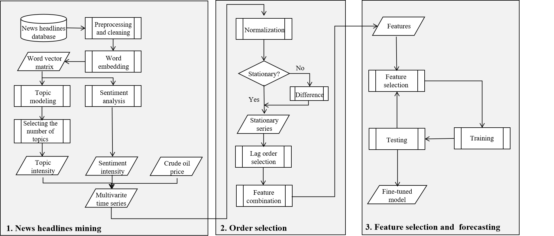
Fig. 3 shows the proposed forecasting framework. Although our work is line with Li et al. 2018, it should be emphasized that this research focuses on point forecasting rather than trend forecasting. We particularly focus on the design and employment of appropriate methods for modelling short and sparse news headlines.
The crude oil forecasting incorporating news text includes three main parts:
- 1.
News headlines mining: the news headlines are first preprocessed, including word segmentation, stop words filtering, stem extraction, etc. Then we use GloVe to do word embedding for the clean texts and get the word vector matrix. Subsequently, topic modelling and sentiment analysis are employed to calculate the topic intensity and sentiment intensity of the futures market.
- 2.
Order selection: we carry out the first-order difference processing for non-stationary time series. We respectively model the interrelationship between each exogenous series with crude oil price series with VAR and obtain the optimal lag. Then we covert multivariate time series forecasting into a regression problem based on these lag value.
- 3.
Feature selection and forecasting: we use RFE to select the most relevant features when constructing the forecasting model. By building a variety of models and comparing rmse, mae, and mape, we finally choose the model that performs best.
To compare the proposed forecasting framework with Li et al. 2018, Table 1 illustrates the similarities and differences of them. We originally plan to use the the same range of data with Li et al. 2018, but we cannot have access to the data as Investing.com deleted earlier news. In the following experiments, to be fair and comparable, we reproduce their method (Li et al. 2018) and apply it to our data as one of our benchmarks.
| Li et al. 2018 | Our forecasting framework | |
| Research objective | Trend forecasting | Point forecasting |
| Date range | Total range: 2009.9.15-2014.7.20 | Total range: 2011.3.29-2019.3.22 |
| Training range: 2012.4.18-2013.10.7 | Training range: 2011.3.29-2016.7.22 | |
| Test range: 2013.10.8-2014.7.20 | Test range: 2016.7.23-2019.3.22 | |
| Data retrieval | Crude oil price series; Crude oil related news headlines; Other data from financial market | Crude oil price series; Futures related news headlines |
| Data preprocessing | 1. Tokenization and stop-words filtering | 1. Tokenization and stop-words filtering |
| 2. Word embedding with Term Frequency – Inverse Document Frequency (TF-IDF) | 2. Word embedding with GloVe | |
| 3. Hodrick-Prescott (HP) smoothing for trend forecasting | 3. Without HP smoothing | |
| News headlines mining | 1. CNN is used to predict the next day’s oil price movement. | 1. We delete this part for the bad classification accuracy of CNN. |
| 2. Discrete and static sentiment of polarity and subjectivity is calculated by TextBlob. | 2. We design a continuous and dynamic sentiment intensity based on an exponential model (see Formula 13). | |
| 3. Latent topics were discovered by LDA from short and sparse news headlines and Dynamic Topic Model (DTM), but DTM is worse for its stable topics. | 3. We employ SeaNMF, a better topic model for short and sparse texts, with the aim at tackling the lack of contextual information. | |
| 4. KL divergence is used to choose the number of topics. | 4. Pointwise Mutual Information (PMI) score was used in our framework. | |
| Lag selection | VAR model | VAR model |
| Feature selection | RFE model | RFE model |
| Price forecasting | Random forest; Support vector regression; Linear regression | Random forest; Support vector regression; arima and arimax; AdaBoost.RT model |
| Evaluation | mae; rmse | rmse; mae; mape; Multi-step forecasting, DM tests, the applications to gold and natural gas support the validity and generalization of our framework. |
4 Application to crude oil price data
4.1 Data collection and description
Investing.com is a world-renowned financial website that provides real-time information and news about thousands of financial investment products, including global stocks, foreign exchange, futures, bonds, funds, and digital currency, as well as a variety of investment tools. We collected 28,220 news headlines through the futures news column on Investing.com as the text data of this study.
We collected oil price daily data from March 29, 2011, to March 22, 2019, on FRED Economic Data, and the news collected also covered this period. The selected base oil is West Texas Intermediate (WTI) crude oil, which is a common type in North America. WTI has become the benchmark of global crude oil pricing due to US military and economic capabilities in the world.
4.2 Experimental design
In order to systematically and comprehensively verify the superiority of our proposed topic and sentiment indicators, Figure 4 presents the framework of our experimental design. Due to time and energy limitation, we just choose some classic and common used methods regrading to the sentiment analysis, topic modelling, and regression models as our candidate sub-models. Thus, the experimental process includes the comparison of the multiple models based on these sub-models.

- (1)
For the sentiment analysis, we choose a widely used sentiment index integrated in TextBlob. We aim to compare its ability to forecast crude oil price with our novel sentiment intensity.
- (2)
In the part of topic modelling, LDA and SeaNMF are compared for short and spare news headlines.
- (3)
The regression models have been introduced separately in Table 2.
| Method | Description |
|---|---|
| rf | rf is a bagging technology that trains multiple decision trees in parallel and outputs the average prediction results of these trees (Liaw et al. 2002). |
| svr | The purpose of svr is to find the optimal decision boundary so that the data points are closest to the hyperplane or the support vectors are all within the boundaries (Drucker et al. 1997). |
| arima | arima is a well-known time series forecasting model. It is a linear equation whose predictors include the lags of the dependent variable and the lags of the forecasting errors (Contreras et al. 2003). |
| arimax | arima is suitable for univariate time series forecasting, while arimax performs well on multivariate analysis (Hyndman 2010). |
4.3 LDA versus SeaNMF topic analysis for short and sparse news headlines
The PMI score is used to compare the performance of LDA and SeaNMF topic models. The higher the PMI score, the better the model performance. We set k from 2 to 10 to calculate the PMI scores in turn. The blue line in Figure 5 represents the PMI value of the SeaNMF, and the black line represents the PMI value of the LDA. It can be seen from the figure that the PMI value of SeaNMF is generally higher than that of LDA and relatively stable. This shows that SeaNMF is better than LDA in extracting topics from news headlines. When , the PMI value of SeaNMF is the highest, indicating that the model works best when the number of topics is 4. As the number of topics increases, the PMI value of LDA shows a decreasing trend and fluctuates greatly. Therefore, we will no longer consider using LDA to extract topics in following experiments.
We select the top 10 keywords from each topic of SeaNMF, as shown in Table 3. From the keywords, we can see that the SeaNMF model can indeed extract different and meaningful topics from the text. The bold font shows that the four topics can be approximately summarized as crude oil, gold, natural gas, and new energy respectively.

| Topic | Keywords |
|---|---|
| 1 | oil crude u.s prices data supply opec asia ahead gains |
| 2 | gold prices fed asia dollar u.s data ahead gains higher |
| 3 | futures gas natural u.s weekly outlook data low weather supply |
| 4 | exclusive says energy new sources trump billion coal pipeline saudi |
4.4 Order selection
After calculating the topic and sentiment intensity, we obtain six time series, including topic 1 to topic 4, sentiment index, and crude oil prices. Then, we respectively model the interrelationship between each exogenous series with crude oil price series with VAR and obtain the optimal lag. The results are shown in Table 4, in which dprice means that the original price series is non-stationary, and changes to stationary after the first order difference. polarity is the sentiment intensity. All the series are shown in Figure 6, and the description of them are listed in Table 5. We can write the regression equation in the following formula where crude prices can be predicted by these lag values.
| (14) |
| Time Series | topic 1 | topic 2 | topic 3 | topic 4 | polarity | dprice |
|---|---|---|---|---|---|---|
| SIC | -13.0595 | -13.4605 | -12.9977 | -13.4579 | -14.3271 | -8.5941 |
| Lag | 7 | 7 | 7 | 7 | 7 | 3 |
| topic 1 | topic 2 | topic 3 | topic 4 | polarity | dprice | |
|---|---|---|---|---|---|---|
| mean | 0.3743 | 0.2835 | 0.1157 | 0.2264 | 0.5077 | 0.5477 |
| median | 0.3559 | 0.2885 | 0.0723 | 0.2175 | 0.5763 | 0.5505 |
| std | 0.1330 | 0.0925 | 0.1341 | 0.1587 | 0.0601 | 0.0748 |
4.5 Feature selection and forecasting
The time series is divided into a training set and a test set as shown in Figure 7. The performance of forecasts up to 3 days ahead is evaluated over the test data.

After obtaining the lag values of the time series, it is intuitive to regard them as independent variables and oil prices as dependent variables to train the regression model. We use RFE to select features and random forest regression (rf), support vector regression (svr), autoregressive integrated moving average (arima), autoregressive integrated moving average with explanatory variable (arimax), the method from Li et al. 2018 (svr-Li) and AdaBoost.RT (ada) to fit the crude oil prices and complete forecasting on the test set. svr-Li is a forecasting model based on svr that combines multi-source text and financial features (Li et al. 2018). At the same time, the rmse, mae, mape between the model with and without text features are compared. Some brief introductions have been listed in Table 2.
| Model | Number of | h=1 | h=2 | h=3 | |||||||
|---|---|---|---|---|---|---|---|---|---|---|---|
| features | rmse | mae | mape | rmse | mae | mape | rmse | mae | mape | ||
| rf | no text | 3 | 0.0728 | 0.0545 | 0.1018 | 0.0742 | 0.0561 | 0.1042 | 0.0744 | 0.0564 | 0.1052 |
| textblob | 36 | 0.0681 | 0.0514 | 0.0971 | 0.0691 | 0.0526 | 0.0989 | 0.0676 | 0.0504 | 0.0947 | |
| our method | 27 | 0.0683 | 0.0520 | 0.0968 | 0.0714 | 0.0542 | 0.1009 | 0.0720 | 0.0531 | 0.0985 | |
| svr | svr-Li | 28 | 0.0646 | 0.0475 | 0.0885 | 0.0602 | 0.0444 | 0.0827 | 0.0603 | 0.0441 | 0.0821 |
| no text | 2 | 0.1111 | 0.1001 | 0.1765 | 0.1116 | 0.0999 | 0.1761 | 0.1116 | 0.1002 | 0.1766 | |
| textblob | 14 | 0.0586 | 0.0427 | 0.0799 | 0.0597 | 0.0442 | 0.0827 | 0.0593 | 0.0428 | 0.0802 | |
| our method | 17 | 0.0584 | 0.0428 | 0.0801 | 0.0596 | 0.0439 | 0.0819 | 0.0593 | 0.0428 | 0.0801 | |
| arima & arimax | no text | – | 0.0565 | 0.0394 | 0.0751 | 0.0566 | 0.0394 | 0.0753 | 0.0566 | 0.0394 | 0.0754 |
| textblob | 23 | 0.0568 | 0.0401 | 0.0757 | 0.0568 | 0.0404 | 0.0759 | 0.0573 | 0.0407 | 0.0765 | |
| our method | 30 | 0.0577 | 0.0412 | 0.0779 | 0.0579 | 0.0417 | 0.0791 | 0.0586 | 0.0422 | 0.0799 | |
| ada | no text | 3 | 0.0594 | 0.0428 | 0.0799 | 0.0599 | 0.0436 | 0.0813 | 0.0602 | 0.0436 | 0.0812 |
| textblob | 7 | 0.0565 | 0.0397 | 0.0751 | 0.0565 | 0.0397 | 0.0752 | 0.0566 | 0.0397 | 0.0751 | |
| our method | 12 | 0.0564 | 0.0396 | 0.0750 | 0.0565 | 0.0396 | 0.0751 | 0.0565 | 0.0396 | 0.0751 | |
The results in Table 6 illustrate the forecasting performance of our proposed method and other benchmarks at horizons 1, 2 and 3. In this table, models named no text are without any text features; models named textblob contain our proposed shore text topic features and use the TextBlob calculation results directly as the sentiment intensity; models named our method contain our proposed short text topic and sentiment features. The general arima and arimax model contains three parameters: p,d and q. p is the number of autoregressive terms, q is the number of sliding average terms, and d is the number of differences taken to make the series stationary. We applied arima (p,d,q) on no text and The arimax (p,d,q) on textblob and our method. The parameters are arima (4,0,3), arimax (4,1,3), and arimax (4,1,3) for no text, textblob, and our method respectively. The text features selected by our method are listed in the Appendix Appendix, from which we can learn the preferences of different models for features. From the results, we can draw conclusions:
- (1)
Text vs no text. For rf, svr, and ada, our method performs better, which also proves that the attempt to add text features to the forecasting model is meaningful. On the other hand, text features are unlikely to improve forecasting accuracy for arima.
- (2)
Our sentiment index vs TextBlob. By comparing the results of textblob and our method, we find that our method is slightly superior to the textblob model in terms of svr and ada. This shows that our proposed sentiment index is better in certain circumstances.
- (3)
Our method vs svr-Li (Li et al. 2018). svr-Li is a forecasting model where the authors use multi-source text and financial features to forecast price. During this period our proposed method deeply extracts short textual features with less human intervention compared to svr-Li. The forecasting improvement of our proposed approach is indeed caused by the several modifications including text source expansion, a more fine word embedding method Glove, SeaNMF short text topic model, continuous sentiment intensity, and the Adaboost.RT model.
- (4)
Optimal Model. The performance of ada is generally better than the other models in terms of rmse and mape. It should be emphasized that the arima model without text features also performs well. We recommend arima to users who can’t get text features. For those who pursue higher forecasting accuracy, we suggest using the proposed method.
4.6 DM significance tests
In this part, we carry out Diebold-Mariano (DM) test (Harvey et al. 1997) to explore that if regression models combined with our proposed text indexes are significantly better or worse than methods like commonly used TextBlob and svr-Li (Li et al. 2018). The null hypothesis is that the two methods have the same forecast accuracy. The alternative hypothesis is that our method is less or more accurate than the standard method. Given a significance level (eg,. 5%), if the DM test statistic falls in the lower or upper 2.5% tail of a standard normal distribution, we reject the null hypothesis. The DM test is implemented using forecast::dm.test() in R.
| svr-Li | ||||||||
|---|---|---|---|---|---|---|---|---|
| h=1 | h=2 | h=3 | h=1 | h=2 | h=3 | |||
| our text index | rf | better | 1.0000 | 1.0000 | 1.0000 | 0.5499 | 0.9219 | 0.9543 |
| rf | worse | 0.0000 | 0.0000 | 0.0000 | 0.4501 | 0.0781 | 0.0457 | |
| our text index | svr | better | 0.0121 | 0.1471 | 0.0203 | 0.2999 | 0.3466 | 0.4375 |
| svr | worse | 0.9879 | 0.8529 | 0.9797 | 0.7001 | 0.6534 | 0.5625 | |
| our text index | arimax | better | 0.0014 | 0.0006 | 0.9994 | 0.8769 | 0.9389 | 1.0000 |
| arimax | worse | 0.9986 | 0.9993 | 0.0006 | 0.1231 | 0.0611 | 0.0000 | |
| our text index | ada | better | 0.0000 | 0.0001 | 0.0000 | 0.7348 | 0.9986 | 0.8603 |
| ada | worse | 1.0000 | 0.9999 | 1.0000 | 0.2652 | 0.0014 | 0.1397 | |
We can observe that
- (1)
Regression methods such as svr, arimax and ada combined with our proposed index are significantly better than svr-Li (Li et al. 2018), indicating our methods only use text features without considering any extra financial features, yielding better forecasts.
- (2)
Results also show that our method is neither significantly better nor worse than textblob. Our proposed topic intensity still needs to be re-designed and optimized in the future study.
Next, in order to identify the optimal model, we further want to validate if ada with our proposed text index is significantly better than other regression methods. We conclude that
- (1)
ada combined with our proposed text index is significantly better than other regression models except for arimax over h=1.
- (2)
On the other hand, it is interesting that ada is not significantly worse than other all models.
| rf | svr | arimax | ||||||||
|---|---|---|---|---|---|---|---|---|---|---|
| h=1 | h=2 | h=3 | h=1 | h=2 | h=3 | h=1 | h=2 | h=3 | ||
| ada | better | 0.0000 | 0.0000 | 0.0000 | 0.0001 | 0.0000 | 0.0001 | 0.0112 | 0.0051 | 0.0000 |
| worse | 1.0000 | 1.0000 | 1.0000 | 0.9999 | 1.0000 | 0.9999 | 0.9888 | 0.9949 | 1.0000 | |
5 Application to natural gas and gold price data
In section 3, we briefly discussed the relationships among the three futures prices of crude oil, natural gas, and gold based on previous research. Since our method incorporating news headlines can forecast crude oil prices pretty well, it’s intuitive that it can also be migrated to other application scenarios. That is, our method may be used to forecast the prices of natural gas and gold. It should be emphasized that since (Li et al. 2018) only forecast crude oil prices and the experimental results in the previous section have verified that our method is more advanced than svr-li, we do not include svr-li in the comparison in this section for the price forecasts of natural gas and gold. And textblob is no longer considered in this scenario either.
5.1 Application to natural gas price data
| Time Series | topic 1 | topic 2 | topic 3 | topic 4 | polarity | dprice |
|---|---|---|---|---|---|---|
| SIC | -12.4214 | -12.8220 | -12.3614 | -12.8161 | -13.6855 | -7.9601 |
| lag | 7 | 7 | 7 | 8 | 7 | 3 |
| Model | Number of | h=1 | h=2 | h=3 | |||||||
|---|---|---|---|---|---|---|---|---|---|---|---|
| features | rmse | mae | mape | rmse | mae | mape | rmse | mae | mape | ||
| rf | no text | 3 | 0.0661 | 0.0430 | 0.1349 | 0.0662 | 0.0433 | 0.1382 | 0.0664 | 0.0428 | 0.1406 |
| our method | 28 | 0.0630 | 0.0401 | 0.1355 | 0.0582 | 0.0350 | 0.1237 | 0.0585 | 0.0349 | 0.1235 | |
| svr | no text | 3 | 0.0587 | 0.0354 | 0.1226 | 0.0592 | 0.0357 | 0.1237 | 0.0586 | 0.0352 | 0.1223 |
| our method | 8 | 0.0585 | 0.0352 | 0.1237 | 0.0582 | 0.0350 | 0.1237 | 0.0585 | 0.0349 | 0.1235 | |
| arima & arimax | no text | – | 0.0581 | 0.0348 | 0.1222 | 0.0581 | 0.0348 | 0.1224 | 0.0581 | 0.0348 | 0.1223 |
| our method | 30 | 0.0581 | 0.0350 | 0.1232 | 0.0585 | 0.0357 | 0.1240 | 0.0587 | 0.0353 | 0.1231 | |
| ada | no text | 3 | 0.0581 | 0.0347 | 01224 | 0.0581 | 0.0348 | 0.1225 | 0.0581 | 0.0347 | 0.1225 |
| our method | 19 | 0.0581 | 0.0347 | 0.1222 | 0.0581 | 0.0347 | 0.1224 | 0.0581 | 0.0346 | 0.1224 | |
Analogously, we first calculate the lag of the natural gas-related time series, as shown in Table 9. The parameters of p, d, q are arima (3,0,4) for no text and arimax (4,1,2) for our method. From Table 10, conclusions similar to those in Section 4.5 can be obtained. For the rf, svr and ada , our approach shows its superiority over no text and performs best on ada. However, the arimax model, which uses our proposed text features, does not significantly outperform the arima model.
5.2 Application to gold price data
| Time Series | topic 1 | topic 2 | topic 3 | topic 4 | polarity | dprice |
|---|---|---|---|---|---|---|
| SIC | -12.6794 | -12.6277 | -12.6198 | -13.0770 | -13.9493 | -8.2163 |
| lag | 7 | 7 | 7 | 7 | 7 | 4 |
| Model | Number of | h=1 | h=2 | h=3 | |||||||
|---|---|---|---|---|---|---|---|---|---|---|---|
| features | rmse | mae | mape | rmse | mae | mape | rmse | mae | mape | ||
| rf | no text | 4 | 0.0528 | 0.0367 | 0.0562 | 0.0539 | 0.0385 | 0.0591 | 0.0516 | 0.0367 | 0.0563 |
| our method | 40 | 0.0507 | 0.0353 | 0.0545 | 0.0517 | 0.0362 | 0.0558 | 0.0504 | 0.0359 | 0.0555 | |
| svr | no text | 4 | 0.0452 | 0.0299 | 0.0460 | 0.0460 | 0.0308 | 0.0474 | 0.0456 | 0.0302 | 0.0465 |
| our method | 4 | 0.0467 | 0.0319 | 0.0498 | 0.0471 | 0.0323 | 0.0504 | 0.0474 | 0.0323 | 0.0504 | |
| arima | no text | – | 0.0449 | 0.0292 | 0.0451 | 0.0449 | 0.0293 | 0.0452 | 0.0449 | 0.0293 | 0.0451 |
| our method | 11 | 0.0450 | 0.0296 | 0.0456 | 0.0454 | 0.0303 | 0.0463 | 0.0452 | 0.0296 | 0.0459 | |
| ada | no text | 4 | 0.0449 | 0.0292 | 0.0450 | 0.0449 | 0.0293 | 0.0451 | 0.0449 | 0.0293 | 0.0451 |
| our method | 15 | 0.0447 | 0.0292 | 0.0451 | 0.0449 | 0.0293 | 0.0451 | 0.0447 | 0.0293 | 0.0451 | |
The parameters of p,d,q are arima (4,1,3) for no text and arimax (3,2,1) for our method. From Table 12, our method only outperforms no text on rf. Thus, it can be seen that the proposed textual features have a less significant role in improving the forecasting accuracy of gold prices. We conjecture that this is due to the low discussion of gold in all news text.
6 Discussion
The international crude oil prices are influenced by many external factors in addition to historical price fluctuations, making the accurate and reliable forecasting a difficult task. The empirical results in Demirer & Kutan 2010 and Kaiser & Yu 2010 suggest that incorporating UCG information from the social media into the crude oil price forecasting can achieve better performance. In order to obtain higher accuracy, researchers are free to add more various exogenous variables to their forecasting framework, such as Li et al. 2018. Although these exogenous variables can boost the forecasting ability to some extent, they also bring some uncertainty in forecasting due to excessive human intervention. What’s more, their work does not systematically examine whether textual features or these exogenous features lead to good predictions. In this work, we suggest a change from adding more exogenous variables to construct high quality features from short and sparse text and mitigate the importance of manual intervention. Our study focuses on extracting as much information as possible from news headlines to assist in forecasting crude oil prices, without manually choosing many other exogenous variables, yielding comparable performance.
Specifically, to fully extract features from short and sparse news headlines, we employ advanced GloVe instead of bag of words during word embedding as GloVe’s pretrained model makes full use of massive corpus information, retains more semantic relationships, and saves considerable time while bag of words focuses more on syntax than on semantics.
For topic modelling, LDA is designed for accommodating long text and has been used in Li et al. 2018. However, news headlines are short and sparse, making traditional LDA difficult to discover potential topics from them due to the lack of contextual information (Shi et al. 2018). This mismatch between the text and topic model directly has a bad influence on the forecasting performance. Considering that, we employ advanced short text model SeaNMF to construct topic intensity, with the aim at tackling the short and sparse news headlines and thus improving the forecasting performance. Our empirical results also show that SeaNMF is more suitable to infer potential topics for the short and sparse news headlines than LDA.
In terms of sentiment analysis, the sentiment indicator constructed in Li et al. 2018 is static and simple, ignoring the dynamic relationship with the previous days. So we design a novel sentiment indicator, taking the cumulative and diminishing effect of the market into consideration.
Our empirical results prove that the proposed two marketing indicators are systematically combined with other key factors and thus produce more accurate forecasts compared with (Li et al. 2018). DM significance tests show that regression models such as svr, arimax and ada combined with our proposed text indexes are significantly better than state-of-the-art svr-Li (Li et al. 2018), indicating that our methods produce better forecasts with fewer human intervention. Also, it is interesting that our proposed sentiment indicator is neither significantly better or worse than methods combined with TextBlob. We further verify the superiority of ada combined with the proposed text indicators with others.
Another significant merit is that our forecasting framework can also yield good forecasting performance when applied to other futures commodities, reflecting the flexibility and robustness of it. Due to the use of futures-related news headlines as an experimental training corpus, our method also obtains the expected good results in forecasting the prices of natural gas and gold. In future, the research framework can be transferred to other fields. For example, the news text features of listed companies can be added to the model to enhance the accuracy of its stock price prediction.
The limitation of this study is that it extracts text features from two dimensions, topic and sentiment, which can be further fully obtained by adding additional perspectives such as news categories, distribution and density. In the future, comments on the news from investors or other people who pay attention to crude oil could also be considered in our framework.
7 Concluding remarks
Inspired by the work (Li et al. 2018), where they construct text indicators from news headlines and add some exogenous financial features to their forecasting model, we have reproduced their experimental process, studied their ideas in depth, and proposed some modifications and innovations. To improve forecasting performance, we particularly focus on the modelling for sparse and short news headlines. Two novel indicators based on sparse and short text are combined with other models and produce good performance. Applying the proposed approaches in natural gas and gold price forecasting is a strong support of the validity and generalizability of the research.
Our research framework provides an automated tool for crude oil price forecasting. As far as its practical application is concerned, our method is more suitable for price forecasting with a large amount of historical data. It is even better if there are corresponding news in the past period, as text features can be extracted from them to help improve the prediction. Also, our research focuses more on extracting text features from two dimensions, topic and sentiment, which can be further fully obtained by adding additional perspectives such as news categories, distribution and density.
Acknowledgements
We are grateful to the Editor, two anonymous reviewers for their helpful comments that improved the contents of this paper. We are also grateful to Professor Yanfei Kang from Beihang Univeristy for her meaningful suggestions and insights of this paper.
Appendix
Experimental setup and feature selection results for the crude oil forecasting
- •
Parameters for random forest regression: , , , ;
- •
Parameters for support vector regression: , ;
- •
Parameters for AdaBoost.RT: , , and the base estimator is “DecisionTreeRegressor".
| features | rf-text (27) | svr-text (17) | arimax (4,1,3) (3) | ada-text (12) |
|---|---|---|---|---|
| topic1(t-7) | ✓ | ✓ | ||
| topic1(t-6) | ||||
| topic1(t-5) | ||||
| topic1(t-4) | ✓ | |||
| topic1(t-3) | ✓ | ✓ | ✓ | |
| topic1(t-2) | ||||
| topic1(t-1) | ✓ | ✓ | ✓ | |
| topic2(t-7) | ✓ | |||
| topic2(t-6) | ||||
| topic2(t-5) | ✓ | |||
| topic2(t-4) | ✓ | ✓ | ✓ | |
| topic2(t-3) | ✓ | |||
| topic2(t-2) | ✓ | |||
| topic2(t-1) | ✓ | ✓ | ✓ | ✓ |
| topic3(t-7) | ✓ | ✓ | ||
| topic3(t-6) | ✓ | ✓ | ||
| topic3(t-5) | ||||
| topic3(t-4) | ✓ | |||
| topic3(t-3) | ✓ | |||
| topic3(t-2) | ✓ | ✓ | ||
| topic3(t-1) | ✓ | |||
| topic4(t-7) | ||||
| topic4(t-6) | ||||
| topic4(t-5) | ✓ | ✓ | ✓ | |
| topic4(t-4) | ✓ | |||
| topic4(t-3) | ✓ | ✓ | ||
| topic4(t-2) | ✓ | |||
| topic4(t-1) | ||||
| polarity(t-7) | ✓ | ✓ | ✓ | |
| polarity(t-6) | ✓ | ✓ | ✓ | |
| polarity(t-5) | ✓ | ✓ | ✓ | ✓ |
| polarity(t-4) | ||||
| polarity(t-3) | ✓ | ✓ | ||
| polarity(t-2) | ||||
| polarity(t-1) | ✓ | |||
| dprice(t-3) | ✓ | ✓ | ✓ | |
| dprice(t-2) | ✓ | ✓ | ✓ | |
| dprice(t-1) | ✓ | ✓ | ✓ | ✓ |
| features | rf-text (28) | svr-text (8) | arimax (4,1,2)(30) | ada-text (19) |
|---|---|---|---|---|
| topic1(t-7) | ✓ | ✓ | ||
| topic1(t-6) | ||||
| topic1(t-5) | ✓ | ✓ | ✓ | ✓ |
| topic1(t-4) | ||||
| topic1(t-3) | ✓ | ✓ | ||
| topic1(t-2) | ✓ | ✓ | ||
| topic1(t-1) | ||||
| topic2(t-7) | ✓ | ✓ | ✓ | |
| topic2(t-6) | ✓ | ✓ | ||
| topic2(t-5) | ✓ | ✓ | ||
| topic2(t-4) | ✓ | ✓ | ||
| topic2(t-3) | ✓ | ✓ | ✓ | |
| topic2(t-2) | ✓ | ✓ | ✓ | |
| topic2(t-1) | ✓ | |||
| topic3(t-7) | ✓ | ✓ | ✓ | ✓ |
| topic3(t-6) | ✓ | ✓ | ✓ | |
| topic3(t-5) | ||||
| topic3(t-4) | ||||
| topic3(t-3) | ✓ | ✓ | ✓ | |
| topic3(t-2) | ||||
| topic3(t-1) | ✓ | ✓ | ✓ | ✓ |
| topic4(t-8) | ✓ | ✓ | ✓ | ✓ |
| topic4(t-7) | ✓ | ✓ | ||
| topic4(t-6) | ✓ | ✓ | ✓ | |
| topic4(t-5) | ✓ | ✓ | ||
| topic4(t-4) | ✓ | ✓ | ||
| topic4(t-3) | ✓ | ✓ | ||
| topic4(t-2) | ||||
| topic4(t-1) | ✓ | ✓ | ||
| polarity(t-7) | ✓ | ✓ | ✓ | ✓ |
| polarity(t-6) | ✓ | ✓ | ✓ | |
| polarity(t-5) | ✓ | ✓ | ✓ | |
| polarity(t-4) | ||||
| polarity(t-3) | ✓ | ✓ | ✓ | |
| polarity(t-2) | ||||
| polarity(t-1) | ✓ | ✓ | ✓ | ✓ |
| dprice(t-3) | ✓ | ✓ | ✓ | ✓ |
| dprice(t-2) | ✓ | ✓ | ✓ | |
| dprice(t-1) | ✓ | ✓ | ✓ | ✓ |
| features | rf-text (31) | svr-text (3) | arimax (3,2,1) (24) | ada-text (5) |
| topic1(t-7) | ✓ | ✓ | ||
| topic1(t-6) | ✓ | ✓ | ||
| topic1(t-5) | ✓ | ✓ | ||
| topic1(t-4) | ✓ | ✓ | ||
| topic1(t-3) | ✓ | |||
| topic1(t-2) | ||||
| topic1(t-1) | ✓ | |||
| topic2(t-7) | ✓ | ✓ | ||
| topic2(t-6) | ✓ | |||
| topic2(t-5) | ✓ | ✓ | ||
| topic2(t-4) | ||||
| topic2(t-3) | ✓ | ✓ | ✓ | |
| topic2(t-2) | ✓ | |||
| topic2(t-1) | ✓ | ✓ | ||
| topic3(t-7) | ✓ | ✓ | ||
| topic3(t-6) | ✓ | |||
| topic3(t-5) | ||||
| topic3(t-4) | ✓ | |||
| topic3(t-3) | ✓ | |||
| topic3(t-2) | ✓ | |||
| topic3(t-1) | ✓ | |||
| topic4(t-7) | ✓ | ✓ | ||
| topic4(t-6) | ✓ | ✓ | ||
| topic4(t-5) | ||||
| topic4(t-4) | ✓ | ✓ | ||
| topic4(t-3) | ✓ | ✓ | ||
| topic4(t-2) | ✓ | |||
| topic4(t-1) | ✓ | ✓ | ✓ | ✓ |
| polarity(t-7) | ✓ | ✓ | ||
| polarity(t-6) | ✓ | ✓ | ||
| polarity(t-5) | ✓ | ✓ | ||
| polarity(t-4) | ✓ | |||
| polarity(t-3) | ✓ | |||
| polarity(t-2) | ✓ | ✓ | ||
| polarity(t-1) | ||||
| dprice(t-4) | ✓ | ✓ | ||
| dprice(t-3) | ✓ | ✓ | ||
| dprice(t-2) | ✓ | ✓ | ✓ | ✓ |
| dprice(t-1) | ✓ | ✓ | ✓ | ✓ |
References
- Aggarwal & Zhai (2012) Aggarwal, C. C., & Zhai, C. (2012). Mining text data. Springer Science & Business Media.
- Bernabe et al. (2012) Bernabe, A., Martina, E., Alvarez-Ramirez, J., & Ibarra-Valdez, C. (2012). A multi-model approach for describing crude oil price dynamics. Physica A Statistical Mechanics and Its Applications, 338, 567–584.
- Berry & Castellanos (2004) Berry, M. W., & Castellanos, M. (2004). Survey of text mining. Computing Reviews, 45, 548.
- Blei et al. (2003) Blei, D. M., Ng, A. Y., & Jordan, M. I. (2003). Latent dirichlet allocation. Journal of machine Learning research, 3, 993–1022.
- Chen et al. (2011) Chen, M., Jin, X., & Shen, D. (2011). Short text classification improved by learning multi-granularity topics. In Twenty-Second International Joint Conference on Artificial Intelligence.
- Contreras et al. (2003) Contreras, J., Espinola, R., Nogales, F. J., & Conejo, A. J. (2003). Arima models to predict next-day electricity prices. IEEE transactions on power systems, 18, 1014–1020.
- Deerwester et al. (1990) Deerwester, S., Dumais, S. T., Furnas, G. W., Landauer, T. K., & Harshman, R. (1990). Indexing by latent semantic analysis. Journal of the American society for information science, 41, 391–407.
- Demirer & Kutan (2010) Demirer, R., & Kutan, A. M. (2010). The behavior of crude oil spot and futures prices around opec and spr announcements: An event study perspective. Energy Economics, 32, 1467–1476.
- Drucker et al. (1997) Drucker, H., Burges, C. J., Kaufman, L., Smola, A. J., & Vapnik, V. (1997). Support vector regression machines. In Advances in neural information processing systems (pp. 155–161).
- Ekinci et al. (2015) Ekinci, A., Erdal, H. et al. (2015). Optimizing the monthly crude oil price forecasting accuracy via bagging ensemble models. Journal of Economics and International Finance, 7, 127–136.
- Elshendy et al. (2018) Elshendy, M., Colladon, A. F., Battistoni, E., & Gloor, P. A. (2018). Using four different online media sources to forecast the crude oil price. Journal of Information Science, 44, 408–421.
- Gumus & Kiran (2017) Gumus, M., & Kiran, M. S. (2017). Crude oil price forecasting using xgboost. In 2017 International Conference on Computer Science and Engineering (UBMK) (pp. 1100–1103). IEEE.
- Guyon et al. (2002) Guyon, I., Weston, J., Barnhill, S., & Vapnik, V. (2002). Gene selection for cancer classification using support vector machines. Machine learning, 46, 389–422.
- Hagen (2010) Hagen, R. (2010). How is the international price of particular crude determined? Opec Energy Review, 18, 127–135.
- Harvey et al. (1997) Harvey, D., Leybourne, S., & Newbold, P. (1997). Testing the equality of prediction mean squared errors. International Journal of forecasting, 13, 281–291.
- Hou & Suardi (2012) Hou, A., & Suardi, S. (2012). A nonparametric garch model of crude oil price return volatility. Energy Economics, 34, 618–626.
- Hyndman (2010) Hyndman, R. J. (2010). The arimax model muddle. Blog. https://robjhyndman. com/hyndsight/arimax, .
- Ivanov & Kilian (2005) Ivanov, V., & Kilian, L. (2005). A practitioner’s guide to lag order selection for var impulse response analysis. Studies in Nonlinear Dynamics & Econometrics, 9.
- Jin et al. (2011) Jin, O., Liu, N. N., Zhao, K., Yu, Y., & Yang, Q. (2011). Transferring topical knowledge from auxiliary long texts for short text clustering. In Proceedings of the 20th ACM international conference on Information and knowledge management (pp. 775–784). ACM.
- Jun et al. (2009) Jun, W., Zhi-bin, L., Qiong, S. et al. (2009). Oil price forcasting based on hierarchical support vector machine [j]. Computer Applications of Petroleum, 63, 5–8.
- Kaiser & Yu (2010) Kaiser, M. J., & Yu, Y. (2010). The impact of hurricanes gustav and ike on offshore oil and gas production in the gulf of mexico. Applied Energy, 87, 284–297.
- Kaur & Sharma (2020) Kaur, C., & Sharma, A. (2020). Twitter Sentiment Analysis on Coronavirus using Textblob. Technical Report EasyChair.
- Kunal et al. (2018) Kunal, S., Saha, A., Varma, A., & Tiwari, V. (2018). Textual dissection of live twitter reviews using naive bayes. Procedia computer science, 132, 307–313.
- Li et al. (2018) Li, X., Shang, W., & Wang, S. (2018). Text-based crude oil price forecasting: A deep learning approach. International Journal of Forecasting, .
- Liaw et al. (2002) Liaw, A., Wiener, M. et al. (2002). Classification and regression by randomforest. R news, 2, 18–22.
- Ling et al. (2015) Ling, T., Wei, D., Yu, L., & Wang, S. (2015). A novel ceemd-based eelm ensemble learning paradigm for crude oil price forecasting. International Journal of Information Technology and Decision Making, 14, 141–169.
- Lütkepohl (2005) Lütkepohl, H. (2005). New introduction to multiple time series analysis. Springer Science & Business Media.
- Mazarura et al. (2015) Mazarura, J. R. et al. (2015). Topic modelling for short text. Ph.D. thesis University of Pretoria.
- Mikolov et al. (2013) Mikolov, T., Chen, K., Corrado, G., & Dean, J. (2013). Efficient estimation of word representations in vector space. arXiv preprint arXiv:1301.3781, .
- Mohammadi & Su (2010) Mohammadi, H., & Su, L. (2010). International evidence on crude oil price dynamics: Applications of arima-garch models. Energy Economics, 32, 1001–1008.
- Moshiri & Foroutan (2006) Moshiri, S., & Foroutan, F. (2006). Forecasting nonlinear crude oil futures prices. The Energy Journal, (pp. 81–95).
- Movagharnejad et al. (2011) Movagharnejad, K., Mehdizadeh, B., Banihashemi, M., & Kordkheili, M. S. (2011). Forecasting the differences between various commercial oil prices in the persian gulf region by neural network. Energy, 36, 3979–3984.
- Pennington et al. (2014) Pennington, J., Socher, R., & Manning, C. (2014). Glove: Global vectors for word representation. In Proceedings of the 2014 conference on empirical methods in natural language processing (EMNLP) (pp. 1532–1543).
- Qiang et al. (2017) Qiang, J., Chen, P., Wang, T., & Wu, X. (2017). Topic modeling over short texts by incorporating word embeddings. In Pacific-Asia Conference on Knowledge Discovery and Data Mining (pp. 363–374). Springer.
- Quan et al. (2015) Quan, X., Kit, C., Ge, Y., & Pan, S. J. (2015). Short and sparse text topic modeling via self-aggregation. In Twenty-Fourth International Joint Conference on Artificial Intelligence.
- Saha et al. (2017) Saha, S., Yadav, J., & Ranjan, P. (2017). Proposed approach for sarcasm detection in twitter. Indian Journal of Science and Technology, 10, 1–8.
- Serrano-Guerrero et al. (2015) Serrano-Guerrero, J., Olivas, J. A., Romero, F. P., & Herrera-Viedma, E. (2015). Sentiment analysis: A review and comparative analysis of web services. Information Sciences, 311, 18–38.
- Shi et al. (2018) Shi, T., Kang, K., Choo, J., & Reddy, C. K. (2018). Short-text topic modeling via non-negative matrix factorization enriched with local word-context correlations. In Proceedings of the 2018 World Wide Web Conference on World Wide Web (pp. 1105–1114). International World Wide Web Conferences Steering Committee.
- Shriharir & Desai (2015) Shriharir, C., & Desai, A. (2015). A review on knowledge discovery using text classification techniques in text mining. International Journal of Computer Applications, 111, 12–15.
- Solomatine & Shrestha (2004) Solomatine, D. P., & Shrestha, D. L. (2004). Adaboost. rt: a boosting algorithm for regression problems. In 2004 IEEE International Joint Conference on Neural Networks (IEEE Cat. No. 04CH37541) (pp. 1163–1168). IEEE volume 2.
- Stevens (2007) Stevens, P. (2007). The determination of oil prices 1945–1995 : A diagrammatic interpretation. Energy Policy, 23, 861–870.
- Sujit & Kumar (2011) Sujit, K., & Kumar, B. R. (2011). Study on dynamic relationship among gold price, oil price, exchange rate and stock market returns. International journal of applied business and economic research, 9, 145–165.
- Villar & Joutz (2006) Villar, J. A., & Joutz, F. L. (2006). The relationship between crude oil and natural gas prices. Energy Information Administration, Office of Oil and Gas, (pp. 1–43).
- Wang et al. (2018) Wang, J., Athanasopoulos, G., Hyndman, R. J., & Wang, S. (2018). Crude oil price forecasting based on internet concern using an extreme learning machine. International Journal of Forecasting, 34, 665–677.
- Wang et al. (2004) Wang, S., Yu, L., & Lai, K. K. (2004). A novel hybrid ai system framework for crude oil price forecasting. In Chinese Academy of Sciences Symposium on Data Mining and Knowledge Management (pp. 233–242). Springer.
- Xiang & Zhuang (2013) Xiang, Y., & Zhuang, X. H. (2013). Application of arima model in short-term prediction of international crude oil price. In Advanced Materials Research (pp. 979–982). Trans Tech Publ volume 798.
- Xie et al. (2006) Xie, W., Yu, L., Xu, S., & Wang, S. (2006). A new method for crude oil price forecasting based on support vector machines. In International Conference on Computational Science (pp. 444–451). Springer.
- Xu & Berkely (2014) Xu, S. Y., & Berkely, C. (2014). Stock price forecasting using information from yahoo finance and google trend. UC Brekley, .
- Yu et al. (2005) Yu, L., Wang, S., & Lai, K. (2005). A rough-set-refined text mining approach for crude oil market tendency forecasting. International Journal of Knowledge and Systems Sciences, 2, 33–46.
- Zhang et al. (2015) Zhang, J. L., Zhang, Y. J., & Zhang, L. (2015). A novel hybrid method for crude oil price forecasting. Energy Economics, 49, 649–659.