Constructing Multipartite Bell inequalities from stabilizersPreprint: APS/123-QED
Abstract
Bell inequality with self-testing property has played an important role in quantum information field with both fundamental and practical applications. However, it is generally challenging to find Bell inequalities with self-testing property for multipartite states and actually there are not many known candidates. In this work, we propose a systematical framework to construct Bell inequalities from stabilizers which are maximally violated by general stabilizer states, with two observables for each local party. We show that the constructed Bell inequalities can self-test any stabilizer state which is essentially device-independent, if and only if these stabilizers can uniquely determine the state in a device-dependent manner. This bridges the gap between device-independent and device-dependent verification methods. Our framework can provide plenty of Bell inequalities for self-testing stabilizer states. Among them, we give two families of Bell inequalities with different advantages: (1) a family of Bell inequalities with a constant ratio of quantum and classical bounds using correlations, (2) Single pair inequalities improving on all previous robustness self-testing bounds using correlations, which are both efficient and suitable for realizations in multipartite systems. Our framework can not only inspire more fruitful multipartite Bell inequalities from conventional verification methods, but also pave the way for their practical applications.
Introduction.— Bell inequalities, as a test for quantum correlations, can distinguish quantum physics from its classical counterpart Bell 1987; Brunner et al. 2014. They not only play a fundamental role in quantum physics, but also demonstrate practical applications in quantum information processing, such as the quantum key distribution Mayers and Yao 1998; Vazirani and Vidick 2014; Miller and Shi 2014; Arnon-Friedman et al. 2018, quantum randomness generation Colbeck 2006; Pironio et al. 2010; Ma et al. 2016; Acín and Masanes 2016; Liu et al. 2018; Bierhorst et al. 2018, blind quantum computing Reichardt et al. 2013; Huang et al. 2017, and quantum resource detection Moroder et al. 2013; Liang et al. 2015; Baccari et al. 2017.
One of the most striking applications of Bell inequality is the simultaneous verification of quantum states and measurements, based on the maximal violation of it Mayers and Yao 1998; McKague et al. 2012. The verification only relies on the input and output statistics without the trust of realization of devices, which is different from traditional quantum tomography and other device-dependent methods Vogel and Risken 1989; Paris and Rehacek 2004. This phenomenon is usually referred as self-testing. When the violation of Bell inequality is only close to its maximal quantum value, one can also estimate the fidelity between the underlying state and the target state which is referred as robust self-testing. Tremendous efforts have been made to self-test various types of quantum states Wu et al. 2014; Wu et al. 2016; Coladangelo et al. 2017; Salavrakos et al. 2017; Baccari et al. 2020, and improve robust self-testing performance which is helpful in the realistic implementation McKague et al. 2012; Miller and Shi 2013; Kaniewski 2016.
Even though Bell inequality and self-testing are of fundamental and practical significance, it is generally challenging and not clear to propose Bell inequalities with the self-testing manner, especially for multipartite states, due to the exponentially increase of the dimension of total Hilbert space. Some interesting and inspiring attempts have been made focusing on high-dimensional maximally entangled states Salavrakos et al. 2017, and graph states Scarani et al. 2005; Gühne et al. 2005; Gühne and Cabello 2008; Baccari et al. 2020, nevertheless in Ref. Scarani et al. 2005; Gühne et al. 2005; Gühne and Cabello 2008 the self-testing property is not explored. Ref. Baccari et al. 2020 proposed an inspiring family of Bell inequalities with self-testing manner, which are constructed from the generators of graph states. The ratio of the quantum and classical bounds tends to a constant in an asymptotic case. However, the candidates for the Bell inequality of general stabilizer states with the self-testing manner are still limited and there is also no systematical and concrete framework for the construction of them.
Meanwhile, device-dependent multipartite entanglement witnesses Terhal 2001; Guhne and Toth 2009; Friis et al. 2019 and state verification methods Pallister et al. 2018; Zhu and Hayashi 2019 have been extensively studied with the development of large-scale entanglement preparations Wang et al. 2018; Friis et al. 2018; Gong et al. 2019. Many efforts have been made aiming at graph states or general stabilizer states which are important resources in quantum information processing tasks, e.g. measurement-based quantum computing Raussendorf and Briegel 2001; Raussendorf et al. 2003, quantum routing and quantum networks Kimble 2008; Perseguers et al. 2013. The entanglement witness and the state verification of stabilizer states can be greatly simplified by utilizing the property of stabilizers Tóth and Gühne 2005; Pallister et al. 2018; Hayashi and Morimae 2015; Fujii and Hayashi 2017; Lu et al. 2018; Zhou et al. 2019a; Zhou 2020; Zeng et al. 2019. Focusing on the device-independent scenario, it is thus an interesting open problem to ask whether the same properties can be applied for constructing Bell inequalities.
In this letter, we propose a systematical framework for constructing Bell inequalities with two local observables from stabilizers. We show that the necessary and sufficient condition to realize the self-testing is that a set of stabilizers used in the construction can uniquely determine the state device-dependently, which closes the gap between the device-dependent and -independent verifications. Taking advantage of the framework, we provide more choices of Bell inequalities with self-testing. As applications, two families of Bell inequalities are proposed showing different advantages. For any stabilizer states, we construct Bell inequalities with constant ratio of quantum and classical bounds with a linear number of correlations, improving the result in Baccari et al. 2020. To further enable the robust self-testing, we take 3, 4-qubit GHZ states and cluster states for example. In particular, also with a linear number of correlations, we construct a new type of Bell inequalities, referred as Single pair inequality showing the best known robust self-testing bound, which outperforms Mermin inequality Mermin 1990; Kaniewski 2016 and Bell inequalities proposed in Baccari et al. 2020. As a side result, our Bell inequalities can also serve as device-independent entanglement witness, which provides more alternatives for the entanglement detection in the device-dependent scenario.
Graph states and the stabilizer formalism.— Stabilizer states Gottesman 1997; Nielsen and Chuang 2011 can be transformed from graph states via local unitary operations Hein et al. 2006. Thus in the following we discuss graph states without loss of generality.
A graph state can be defined based on a graph , with vertices set and edges set . Two vertexes , are neighborhood if there is an edge connecting them, and the neighborhood set of vertex is denoted as . Let the qubits take the role of the vertices and the edges represent the operations between the qubits, that is, the Controlled- operation, a graph state can be written as,
| (1) |
where is the eigenstate of the Pauli matrix and is the Controlled- gate, . Hereafter denote the Pauli operators of the qubit . Graph state can be uniquely determined by generators,
| (2) |
which commute with each other and staisfy . that is, the unique eigenstate with eigenvalue for all the generators. As a result, a graph state can also be written as a product of projectors of the generators,
| (3) |
All the other stabilizers can be generated by the multiplication of these generators. The property of stabilizers can be utilized to verify the graph states and construct entanglement witness efficiently Tóth and Gühne 2005; Zhou et al. 2019a.
Constructing Bell inequalities from pairable stabilizers.— For a -party graph state from graph , we label each party with registers . We refer the graph -colorable, if one can label the graph with different colors requiring that there is no pair of adjacent vertices of the same color. According to this definition, we can divide all the vertices into disjoint subsets , such that there is no edge inside each . The smallest is referred as the chromatic number of .
Considering that each vertex owns a generator and the multiplication of generators from different color subsets can induce more measurement settings ( measurement). In this letter, we mainly explore the efficient Bell inequalities with two local observables for each party. Thus, we focus on the stabilizers which are generated by the generators from the same color subset ,
| (4) |
These stabilizers can be represented by tensor product of Pauli operators, , where . For simplicity, we define a sequence to express a stabilizer with when , when , and when . Before showing the construction of Bell inequalities, let us first define a relationship between two stabilizers.
Definition 1.
Two stabilizers , are called pairable, if there exists at least one position such that local operators are anti-commutative, that is, , or .
Note that pairable stabilizers could have more than one anti-commutative position. Thus this definition is different with anti-commutative stabilizers. Hereafter, we use subscript to represent th party and use superscript to represent different stabilizers. Taking advantage of the property of pairable stabilizers of graph state to construct Bell inequalities, we choose two pairable stabilizers and , and one anti-commutative position . For position , we replace the Pauli operators and in the stabilizers and by observables and , respectively. As for all the other positions , we replace and by and , respectively. Consequently, the Bell inequality based on pairable stabilizers and shows as follows.
Lemma 1.
| (5) |
where , , , , are all binary observables. The classical bound for this Bell inequality is and the quantum bound (the maximal quantum value) which can be reached by the graph state .
The quantum bound is fulfilled by taking when , and when . Intuitively, we can choose a lot of stabilizers to construct Bell inequalities. However, sometimes different pairs could have different anti-commutative positions which leads to inconsistent measurement settings. In order to avoid this inconsistency, we define a vertex subset to decide the observables of some specific positions, such as in . We want to combine a lot of stabilizers, and define the set containing all the chosen pairs and as . Note that for different pairs, they can share the same stabilizer, for example we allow . Besides the stabilizers, one can also add other non-pairable stabilizers , . We define the set containing all the stabilizers appearing in and as . For given , , we put some requirements on as follows.
- 1.
For every stabilizers, and , , there exists only one position such that the measurement setting of stabilizers, and in this position are anti-commutative. For other positions , the measurement settings in and are all , .
- 2.
For every stabilizer , the measurements in any position are , .
These requirements are used to prevent the situation where the maximal classical value of Bell correlation exceeds its maximal quantum value. Though this is not strictly forbidden, it would reduce the ratio of quantum and classical bounds in the constructed Bell inequalities. Luckily, one can always find a suitable for the chosen stabilizer set by the following lemma.
Lemma 2.
For any given stabilizer set containing pairable stabilizers, one can always assign the stabilizers of into the paring set and the remaining subset , and then find a suitable satisfying two requirements listed above.
Thus it is generally feasible to construct Bell inequalities from a stabilizer set . In order to make this construction clearer, we show an example of 4-qubit cluster state in FIG. 1. There are also other constructions for this given stabilizers set , here we only give two constructions as examples.

For , with a suitable satisfying the above two requirements, we construct the Bell inequalities for general graph states as follows.
Theorem 1.
| (6) | ||||
where are defined in Lemma 1, and denote the number of elements in sets and , respectively. The quantum bound and the corresponding graph state can reach this maximal quantum value.
Note that novel CHSH-like multipartite Bell inequalities proposed in Baccari et al. 2020 can be seen as special cases of Theorem 1 by choosing all the stabilizers being generators in Eq. (2), that is, , where is the generator asscociated with th vertex. In particular, assuming the first vertex is the one with the largest number of neighbours, , the generators in are assigned into , with .
Sufficient and necessary condition for self-testing.— Besides ruling out the classical hidden variable model, Bell inequalities further provide us a method to verify quantum states in a device-independent manner. Though graph state can reach the maximal quantum value of all Bell inequalities constructed from its stabilizers in Theorem 1, not all these Bell inequalities can verify uniquely. Here in this section, based on the constructed Bell inequalities, we explore the sufficient and necessary condition for the self-testing of graph states.
Definition 2.
Suppose that the Bell inequality , constructed from the stabilizers of , is maximally violated by a state and corresponding local observables , . If up to local isometries, and these local observables are equivalent to the graph state , and when ; when , we say this Bell inequality can self-test graph state .
In the conventional device-dependent verification of graph states, we have the following fact about determining graph state with the trust of measurement devices.
Fact 1.
Gottesman 1997; Nielsen and Chuang 2011 For the device-dependent verification, a set of stabilizer measurements can uniquely determine the state , if and only if it contains independent stabilizers. A set a stabilizers are independent if they can not generate each other by multiplication, and note that any other stabilizers can be generated by independent stabilizers.
Theorem 2.
The family of Bell inequalities proposed in Theorem 1 can self-test the graph state , if and only if the stabilizers in together can determine the graph state .
Via this theorem, we make a close connection between the device-independent and -dependent verifications. If the stabilizers can determine the graph state under the trust of measurement devices, then one can always transform these stabilizers to Bell inequalities and apply it to verify the state without trusting the devices under our framework. Thus any witnesses and state verification methods based on stabilizers could inspire the construction of Bell inequalities.
Applications.— Equipped with the above framework, we exhibit applications via constructing Bell inequalities with various advantages. Note that in this section we only explore Bell inequalities with the self-testing property.
At first, we prefer to select Bell inequalities with a large ratio of quantum and classical bound , which is beneficial for the experimental violation under practical set-ups and can lead to good performance in cryptography tasks Miller and Shi 2014. From Theorem 1, it is clear that the maximal is when in our construction. Utilizing the properly designed multiplications of generators from the graph state, we can construct self-testing Bell inequalities with the maximal ratio for any graph state.
Corollary 1.
For any -party graph state , based on our framework one can construct Bell inequalities using correlations to reach the maximal with self-testing property in the same time.
The proof and detailed constructions are shown in Appendix C. In Ref. Baccari et al. 2020, only asymptotic case (infinity large ) and some special states, for example, GHZ state can reach this ratio . Due to flexible choices of stabilizers, instead of only using generators, our framework provides Bell inequalities with generally larger than the constructions in Baccari et al. 2020, also using linear number of correlations, which are efficient and scalable for practical demonstrations in multipartite system.
Secondly, we also expect that Bell inequalities can show a good performance in the robust self-testing task. In the robust self-testing, one would like to lower bound the state fidelity to the target graph state (under local isometries), only on account of the Bell inequality value which deviates from the maximal quantum value. Benefiting from the flexibility of our construction, one can have many choices of Bell inequalities at hand. We give constructions of some typical examples, 3-qubit and 4-qubit GHZ states, and 4-qubit 1-D cluster state in Table 1, 2 and 3, respectively, with different and . Based on the method in Baccari et al. 2020; Kaniewski 2016, in FIG. 2, we numerically show the performance of them in robust self-testing, and also compare with the Mermin inequality which is widely used for self-testing GHZ state Mermin 1990; Kaniewski 2016. In principle, the robustness analysis can be extended to more qubits and one can explore more possible Bell inequalities via our framework.
| () | ||||
|---|---|---|---|---|
| 4 Baccari et al. 2020 |
| {6} | ||||
| 4 Baccari et al. 2020 |
| 2 Baccari et al. 2020 | {4} | |||
|---|---|---|---|---|
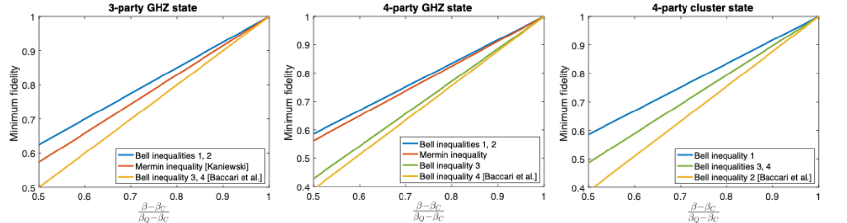
From FIG. 2, one can find that larger value does not necessarily lead to a better performance in the robust self-testing, which is characterized by the slope of the curves. The reason behind this phenomenon may be that the method of estimating fidelity is not tight or optimal. In our examples, we find that the best robust self-testing Bell inequality share the same property, that is, they are constructed from only one pairable stabilizers, i.e., , and other stabilizers all in (See Bell inequality 1 in Table 1, Bell inequalities 1 and 2 in Table 2, Bell inequality 1 in Table 3). We name them as Single pair Bell inequalities,
| (7) |
From these examples and the realizable lower bounds of the fidelity, one can see that our new constructed Single pair Bell inequalities provide the best known robust self-testing bound, improving the previous self-test bound in Kaniewski 2016; Baccari et al. 2020. Note that compared to Mermin inequality with correlations, Single pair Bell inequalities only contains correlations, which is more efficient and scalable for large-scale system verification. This shows the potentiality of our framework.
As a side result of the robust self-testing bound, one can also construct device-independent genuine entanglement witness, by applying the linear self-testing fidelity bound with slope and intercept ,
Corollary 2.
| (8) | ||||
where and are Bell correlations shown in Theorem 1, is the threshold Bell value. The violation of this inequality implies the existence of genuine entanglement.
This corollary is due to the fact that the underlying state possesses genuine entanglement when fidelity with a certain graph state exceeds 0.5 Tóth and Gühne 2005; Zhou et al. 2019a. We give detailed genuine entanglement bounds in Appendix E for our constructed Bell inequalities.
Conclusion— In summary, we propose a systematical framework to construct Bell inequalities directly from stabilizers, and further provide a one-to-one map from the device-dependent verification to the self-testing one.
The framework can provides us a large number of Bell inequalities to select for different application scenarios, for instance, Single pair Bell inequality for robust self-testing. Even though the fidelity lower bounds for robust self-test are obtained by numerics, these result are also instructive for obtaining an (tight) analytical bound for general graph states in the future Kaniewski 2016. One may also find other interesting inequalities with other advantages. Similar to the entanglement witness, a modification of coefficients between different Bell expressions may be beneficial for improving the ratio of quantum and classical bounds and the robust self-testing performance Lu et al. 2018; Zhou et al. 2019a; Zhao et al. 2019.
Via the proposed framework, we close the gap between device-independent and -dependent witness and verification, and borrow the experience from device-dependent study. This connection can inspire more complicated Bell inequalities constructions, for instance, the ones with more than two local measurement, applying operators in stabilizers. It would be also interesting to extend the method to hypergraph state, non-stabilizer states, and high-dimensional entangled states Rossi et al. 2013; Kraft et al. 2018; Bavaresco et al. 2018; Zhou et al. 2019b.
Under the context of entanglement detection, like the entanglement witnesses shown above, one can also obtain device-independent entanglement (structure) witnesses Liang et al. 2015; Lu et al. 2018; Zhou et al. 2019a, and we leave the details in the future work.
Acknowledgement We are grateful to Xiao Yuan for useful discussions. QZ acknowledges the support by the Department of Defense through the Hartree Postdoctoral Fellowship at QuICS. YZ was supported in part by the Templeton Religion Trust under grant TRT 0159.
References
- Bell (1987) J. S. Bell, On the Einstein-Podolsky-Rosen Paradox. Physics 1, 195–200 (1964), Speakable and Unspeakable in Quantum Mechanics (Cambridge University Press, 1987).
- Brunner et al. (2014) N. Brunner, D. Cavalcanti, S. Pironio, V. Scarani, and S. Wehner, Rev. Mod. Phys. 86, 419 (2014).
- Mayers and Yao (1998) D. Mayers and A. Yao, in Proceedings 39th Annual Symposium on Foundations of Computer Science (Cat. No.98CB36280) (1998) pp. 503–509.
- Vazirani and Vidick (2014) U. Vazirani and T. Vidick, Phys. Rev. Lett. 113, 140501 (2014).
- Miller and Shi (2014) C. A. Miller and Y. Shi, in Proceedings of the 46th Annual ACM Symposium on Theory of Computing, STOC ’14 (ACM, New York, NY, USA, 2014) pp. 417–426.
- Arnon-Friedman et al. (2018) R. Arnon-Friedman, F. Dupuis, O. Fawzi, R. Renner, and T. Vidick, Nat. Commun. 9, 459 (2018).
- Colbeck (2006) R. Colbeck, Ph.D. thesis, Trinity College, University of Cambridge (2006).
- Pironio et al. (2010) S. Pironio, A. Acín, S. Massar, A. B. de La Giroday, D. N. Matsukevich, P. Maunz, S. Olmschenk, D. Hayes, L. Luo, T. A. Manning, and C. Monroe, Nature 464, 1021 (2010).
- Ma et al. (2016) X. Ma, X. Yuan, Z. Cao, B. Qi, and Z. Zhang, npj Quantum Inform. 2, 16021 (2016).
- Acín and Masanes (2016) A. Acín and L. Masanes, Nature 540, 213 (2016).
- Liu et al. (2018) Y. Liu, Z. Qi, M.-H. Li, J.-Y. Guan, Y. Zhang, B. Bai, W. Zhang, W.-Z. Liu, C. Wu, X. Yuan, et al., Nature 562, 548 (2018).
- Bierhorst et al. (2018) P. Bierhorst, E. Knill, S. Glancy, Y. Zhang, A. Mink, S. Jordan, A. Rommal, Y.-K. Liu, B. Christensen, S. W. Nam, et al., Nature 556, 223 (2018).
- Reichardt et al. (2013) B. W. Reichardt, F. Unger, and U. Vazirani, Nature 496, 456 (2013).
- Huang et al. (2017) H.-L. Huang, Q. Zhao, X. Ma, C. Liu, Z.-E. Su, X.-L. Wang, L. Li, N.-L. Liu, B. C. Sanders, C.-Y. Lu, and J.-W. Pan, Phys. Rev. Lett. 119, 050503 (2017).
- Moroder et al. (2013) T. Moroder, J.-D. Bancal, Y.-C. Liang, M. Hofmann, and O. Gühne, Phys. Rev. Lett. 111, 030501 (2013).
- Liang et al. (2015) Y.-C. Liang, D. Rosset, J.-D. Bancal, G. Pütz, T. J. Barnea, and N. Gisin, Phys. Rev. Lett. 114, 190401 (2015).
- Baccari et al. (2017) F. Baccari, D. Cavalcanti, P. Wittek, and A. Acín, Phys. Rev. X 7, 021042 (2017).
- McKague et al. (2012) M. McKague, T. H. Yang, and V. Scarani, Journal of Physics A: Mathematical and Theoretical 45, 455304 (2012).
- Vogel and Risken (1989) K. Vogel and H. Risken, Phys. Rev. A 40, 2847 (1989).
- Paris and Rehacek (2004) M. Paris and J. e. Rehacek, in Lect. Notes Phys. (2004), 10.1007/b98673.
- Wu et al. (2014) X. Wu, Y. Cai, T. H. Yang, H. N. Le, J.-D. Bancal, and V. Scarani, Phys. Rev. A 90, 042339 (2014).
- Wu et al. (2016) X. Wu, J.-D. Bancal, M. McKague, and V. Scarani, Phys. Rev. A 93, 062121 (2016).
- Coladangelo et al. (2017) A. Coladangelo, K. T. Goh, and V. Scarani, Nature communications 8, 15485 (2017).
- Salavrakos et al. (2017) A. Salavrakos, R. Augusiak, J. Tura, P. Wittek, A. Acín, and S. Pironio, Phys. Rev. Lett. 119, 040402 (2017).
- Baccari et al. (2020) F. Baccari, R. Augusiak, I. Šupić, J. Tura, and A. Acín, Phys. Rev. Lett. 124, 020402 (2020).
- Miller and Shi (2013) C. A. Miller and Y. Shi, in 8th Conference on the Theory of Quantum Computation, Communication and Cryptography (TQC 2013), Leibniz International Proceedings in Informatics (LIPIcs), Vol. 22, edited by S. Severini and F. Brandao (Schloss Dagstuhl–Leibniz-Zentrum fuer Informatik, Dagstuhl, Germany, 2013) pp. 254–262.
- Kaniewski (2016) J. Kaniewski, Phys. Rev. Lett. 117, 070402 (2016).
- Scarani et al. (2005) V. Scarani, A. Acín, E. Schenck, and M. Aspelmeyer, Phys. Rev. A 71, 042325 (2005).
- Gühne et al. (2005) O. Gühne, G. Tóth, P. Hyllus, and H. J. Briegel, Phys. Rev. Lett. 95, 120405 (2005).
- Gühne and Cabello (2008) O. Gühne and A. Cabello, Phys. Rev. A 77, 032108 (2008).
- Terhal (2001) B. M. Terhal, Linear Algebra and its Applications 323, 61 (2001).
- Guhne and Toth (2009) O. Guhne and G. Toth, Physics Reports 474, 1 (2009).
- Friis et al. (2019) N. Friis, G. Vitagliano, M. Malik, and M. Huber, Nature Reviews Physics 1, 72 (2019).
- Pallister et al. (2018) S. Pallister, N. Linden, and A. Montanaro, Phys. Rev. Lett. 120, 170502 (2018).
- Zhu and Hayashi (2019) H. Zhu and M. Hayashi, Phys. Rev. Lett. 123, 260504 (2019).
- Wang et al. (2018) X.-L. Wang, Y.-H. Luo, H.-L. Huang, M.-C. Chen, Z.-E. Su, C. Liu, C. Chen, W. Li, Y.-Q. Fang, X. Jiang, J. Zhang, L. Li, N.-L. Liu, C.-Y. Lu, and J.-W. Pan, Phys. Rev. Lett. 120, 260502 (2018).
- Friis et al. (2018) N. Friis, O. Marty, C. Maier, C. Hempel, M. Holzäpfel, P. Jurcevic, M. B. Plenio, M. Huber, C. Roos, R. Blatt, and B. Lanyon, Phys. Rev. X 8, 021012 (2018).
- Gong et al. (2019) M. Gong, M.-C. Chen, Y. Zheng, S. Wang, C. Zha, H. Deng, Z. Yan, H. Rong, Y. Wu, S. Li, F. Chen, Y. Zhao, F. Liang, J. Lin, Y. Xu, C. Guo, L. Sun, A. D. Castellano, H. Wang, C. Peng, C.-Y. Lu, X. Zhu, and J.-W. Pan, Phys. Rev. Lett. 122, 110501 (2019).
- Raussendorf and Briegel (2001) R. Raussendorf and H. J. Briegel, Phys. Rev. Lett. 86, 5188 (2001).
- Raussendorf et al. (2003) R. Raussendorf, D. E. Browne, and H. J. Briegel, Phys. Rev. A 68, 022312 (2003).
- Kimble (2008) H. J. Kimble, Nature 453, 1023 EP (2008).
- Perseguers et al. (2013) S. Perseguers, G. J. Lapeyre, D. Cavalcanti, M. Lewenstein, and A. Acín, Reports on Progress in Physics 76, 096001 (2013).
- Tóth and Gühne (2005) G. Tóth and O. Gühne, Phys. Rev. Lett. 94, 060501 (2005).
- Hayashi and Morimae (2015) M. Hayashi and T. Morimae, Phys. Rev. Lett. 115, 220502 (2015).
- Fujii and Hayashi (2017) K. Fujii and M. Hayashi, Phys. Rev. A 96, 030301 (2017).
- Lu et al. (2018) H. Lu, Q. Zhao, Z.-D. Li, X.-F. Yin, X. Yuan, J.-C. Hung, L.-K. Chen, L. Li, N.-L. Liu, C.-Z. Peng, Y.-C. Liang, X. Ma, Y.-A. Chen, and J.-W. Pan, Phys. Rev. X 8, 021072 (2018).
- Zhou et al. (2019a) Y. Zhou, Q. Zhao, X. Yuan, and X. Ma, npj Quantum Information 5, 1 (2019a).
- Zhou (2020) Y. Zhou, Phys. Rev. A 101, 012301 (2020).
- Zeng et al. (2019) P. Zeng, Y. Zhou, and Z. Liu, arXiv:1911.06855 (2019).
- Mermin (1990) N. D. Mermin, Phys. Rev. Lett. 65, 1838 (1990).
- Gottesman (1997) D. Gottesman, arXiv: quant-ph/9705052 (1997).
- Nielsen and Chuang (2011) M. A. Nielsen and I. L. Chuang, Quantum Computation and Quantum Information: 10th Anniversary Edition, 10th ed. (Cambridge University Press, New York, NY, USA, 2011).
- Hein et al. (2006) M. Hein, W. Dür, J. Eisert, R. Raussendorf, M. Van den Nest, and H. J. Briegel, arXiv e-prints , quant-ph/0602096 (2006), arXiv:quant-ph/0602096 [quant-ph] .
- Zhao et al. (2019) Q. Zhao, G. Wang, X. Yuan, and X. Ma, Phys. Rev. A 99, 052349 (2019).
- Rossi et al. (2013) M. Rossi, M. Huber, D. BruB, and C. Macchiavello, New Journal of Physics 15, 113022 (2013).
- Kraft et al. (2018) T. Kraft, C. Ritz, N. Brunner, M. Huber, and O. Gühne, Phys. Rev. Lett. 120, 060502 (2018).
- Bavaresco et al. (2018) J. Bavaresco, N. Herrera Valencia, C. KlMei ckl, M. Pivoluska, P. Erker, N. Friis, M. Malik, and M. Huber, Nature Physics 14, 1032 (2018).
- Zhou et al. (2019b) Y. Zhou, C. Guo, and X. Ma, Phys. Rev. A 99, 052324 (2019b).
- Horodecki et al. (2009) R. Horodecki, P. Horodecki, M. Horodecki, and K. Horodecki, Rev. Mod. Phys. 81, 865 (2009).
Appendix A Proof for Constructed Bell inequalities
Proof for Lemma 1—. For any pairable stabilizers and , we choose one of its anti-commutative position as , such that . It is not hard to see that the classical value of can not be greater than .
Then we prove the quantum bound by expressing the difference as
| (9) |
The quantum bound is reached by choosing and for with the underlying state is the graph state .
Proof for Lemma 2.— We choose one pair of pairable stabilizers and , and choose one anti-commutative position, denoted as . We divide all the stabilizers belonging to into three subsets according to the measurement setting on the th position,
| (10) | ||||
Any stabilizers and are pairable. If , we can reuse the stabilizers. In this way, all the stabilizers in can be assigned into paring set and also let and . The above construction satisfies two listed requirements.
Proof for Theorem 1.— First, the classical bound can be obtained by multiple uses of the result in Lemma 1, that is, and the fact .
Then we prove the quantum bound by showing that
| (11) |
Note that here in each , and all the observables and are not fixed measurement settings, they are arbitrary dichotomic observables. Similar as the proof of Lemma 1, this inequality can be transformed into a sum of the following squares.
| (12) |
| (13) |
The quantum bound is reached by choosing when . when with the underlying state is the graph state .
Appendix B Proof for Self-testing
Proof for Theorem 2.— At first, we prove the “if ” part. We assume the underlying state is and observables are for the th party, and prove that for all correlations in Bell inequality there exists an isometry , with local isometries ,
| (14) |
where for , , ; , for , , .
Without loss of generality, in the following we assume and the case where contains more than one position can be proved similarly. Denote
| (15) |
where are normalized parameters such that . For , we denote and which are the actually implemented observables.
A key step of the proof is to show that for each position , when acting on the underlying state , and are anti-commutative, i.e.,
| (16) |
When the Bell inequality reach the maximal value, the inequalities in Eq. (12) and (13) in the proof of Theorem 1 should be saturated when acting on the state . As a result, according to each square in the equations, we have
| (17) | ||||
where and . For the position , the anticommutive relationship can be obtained directly from Eq. (15),
| (18) |
Since the stabilizers in can determine the graph state , at least contains independent stabilizers. For all generators in Eq. (2), there always exist a series of stabilizers from satisfying
| (19) |
with . By multiple uses of Eq. (17) and plugging into Eq. (19), we have
| (20) |
for all . Thus for , by utilizing the relations of vertex and in Eq. (20), we have
| (21) |
where denotes the set of all the vertexes which are neighbors of either or , but are not or themselves. Starting from position 1, we can obtain the anti-commutative relationship for the positions ,
| (22) |
Then in the same way, we can to obtain the anti-commutative relationship for the operators whose corresponding vertex is the neighbor of the vertexes in . Because the graph is connected, we can iterate the above procedure and get the anti-commutative relationship for all parties. The construction of the isometry is exactly the same with that in Baccari et al. 2020 and we do not repeat it here.
Secondly, we prove the “only if ” part. We assume that there exists a stabilizer set , which can not determine the graph state. That is, it can at most contain independent stabilizers denoted by , and we can always find one generator denoted by which can not be expressed by the product of stabilizers in . Consequently, we construct a state
| (23) |
which is the maximally mixed state in the two dimensional subspace, determined by all taking the eigenvalue 1. As a result, has exactly the same value with for Bell inequalities constructed from . Note that is actually the mixture of and another state,
| (24) | ||||
Here the state is determined by all taking the eigenvalue 1 and taking ,
| (25) |
Since is complete, one can uniquely determine whether or , by multiplying the results of them. And we denote the vertex subset . As a result, can also be transformed from by local unitary,
| (26) |
In the following, we show that can not be transformed to by local isometries, which contradicts to the self-testing claim. Let us focus on any single qubit, say the 1st qubit, and take it as the subsystem , and the remaining qubits as . The quantum conditional entropy on of the state is
| (27) |
where we use the fact that is pure and the entanglement entropy of the first qubit is Hein et al. 2006. On the other hand, quantum conditional entropy of the state shows
| (28) | ||||
where we apply the fact that is a maximally mixed state in the subspace, and the entropy of is upper bounded by the qubit number .
It is known that quantifies how many qubits need to send from (Alice) to (Bob) to reconstruct at Bob’s side in the quantum state merging task Horodecki et al. 2009. A negative value indicates that one does not need to send qubits, but can also gain maximally entangled pairs. Considering the two states given before, suppose one can transform to with local isometries, and we show this is contradict to the quantum state merging efficiency. First, transform to with local isometries, and then one can finish the quantum state merging of without any qubit sending but get one entangled pair. Finally, one can transform back to with local operations according to Eq. (25), which contradicts to .
Appendix C Proof for Applications
Proof for Corollary 1.— We divide the vertices of the graph with chromatic number into disjointed subset . According to Lemma 3 below, one can always find a vertex, without loss of generality, denoted as the vertex belonging to the first color subset, satisfying that from every other color subset , there always exists at least one vertex, such that vertex and are neighbors, i.e., . We construct disjoint stabilizer sets as follows,
| (29) | ||||
where denotes the generator of the th vertex. Here contains and the multiplications of with the other generators from the first color set . For , contains the generators of the neighbors of vertex , and the multiplications of these generators with the other generators from the same color set . For simplicity of the construction, we only consider the multiplication of with one of the generators from , say .
It is not hard to check that any pair of are pairable. In particular, they are anti-commutative at the first position . We denote the stabilizers in as and other stabilizers in as . We choose , and when we construct the corresponding Bell inequality by reusing stabilizer as follows,
| (30) |
where . When , we reuse stabilizer , and construct Bell inequality
| (31) |
These two Bell inequality both has correlations and the maximal quantum values are , , respectively. As the result, the ratio for both cases.
The stabilizers we used are containing independent stabilizers. Via Theorem 2, we prove that the above inequality can self-test the graph state .
Lemma 3.
For any graph whose chromatic number is with disjoint color sets , , there always exists a vertex, for example, satisfying that from every other color subset, we could find at least one vertex such that vertex and are neighbors, .
Proof.
We prove this lemma by contradiction. Assuming that we could not find the vertex satisfying the requirement, we denote the vertex with the maximal different color neighbors as vertex 1. Thus there exists a color set, for example , no vertex from it is neighbor to vertex 1. Then we pick one vertex from , denoted as vertex , we can always find a color set such that every vertex in is not neighbor to , otherwise it is contradictive to the assumption that vertex 1 has the maximal different color neighbors. Then we can color this vertex with color . Repeat this procedure for the vertices in color set and we find that this graph can be colored with color, which causes a contradiction. ∎
Appendix D Robust self-test of graph state
In this section, we give the detailed explanation about numerical robustness results of self-testing shown in FIG 2. We would like to lower bound the fidelity between the measured state and the target graph state (under local isometry), with the knowledge of the Bell inequality value. To this end, mathematical equivalently, one can adopt local extraction channel and the maximal fidelity shows
| (32) |
where is the local channel on -th party. Alternatively, the fidelity can be written as follows,
| (33) |
where is the dual channel of . Note that here the dual of the extraction map acts on the graph state, and we denote the state after this dual channel as .
To find a reliable lower bound of the fidelity from the Bell inequality value, one can choose appropriate parameters and such that the following inequality on operators always holds,
| (34) |
where is Bell inequality to self-test the state. In this way, the fidelity is bounded as , with the Bell inequality value.
Since the measurement of is restricted to the dichotomic scenario, on account of the Jordan lemma, one can reduce the state to the N-qubit space, and the possible measurements can be parameterized by the angles as,
| (35) | ||||
for , the rotated set, and for other qubits
| (36) | ||||
where . Consider a specific extraction channel in Ref. Kaniewski 2016,
| (37) |
where , and is the operator on -th qubit: for , as ; for , as . Now the Bell inequality and the operator are both parameterized with , and the inequality in Eq. (34) shows,
| (38) |
where we should find an optimal and for all possible .
In FIG. 2, all the robustness results for 3, 4-partite GHZ or cluster states are obtained from the above inequality numerically. To be specific, given a fixed , we find the minima of the minimal eigenvalue of for all . A slower slope indicates a better bound. Thus, to find the optimal linear bound, we let the relation hold, that is, the fidelity approaches for the maximal quantum value and find the minimum . We list all the obtained and in FIG. 2 as follows.
| 3-qubit GHZ (cluster) | ||
|---|---|---|
| & | 0.906 | -2.4686 |
| & | 0.6036 | -2.4145 |
| Mermin Kaniewski 2016 |
| 4-qubit GHZ | ||
|---|---|---|
| & | 1 | |
| 0.69 | -3.5931 | |
| 0.49 | -3.1578 | |
| Mermin | 0.219 | -0.752 |
| 4-qubit cluster | ||
|---|---|---|
| 1 | ||
| 0.7400 | -3.9262 | |
| & | 0.6200 | -2.5071 |
Appendix E Device-independent Entanglement Witness
As a side result of the robust self-testing bound, applying the linear self-testing bound shown above, we can also construct device-independent entanglement witness. In the following, we give genuine entanglement bounds and the detailed construction for Single pair inequality with the best known robustness bound. The device-independent genuine entanglement witness of 3-party, 4-party GHZ and 4-party cluster are shown, respectively. Any violation of these inequalities implies the existence of genuine entanglement and the similar method can also be used to detect more detailed entanglement structures in a device-independent manner.
| (39) | ||||