The Fundamental Performance of FAST with 19-beam Receiver at L Band
Abstract
The Five-hundred-meter Aperture Spherical radio Telescope (FAST) passed national acceptance and is taking pilot cycle of ‘Shared-Risk’ observations. The 19-beam receiver covering 1.05-1.45 GHz was used for most of these observations. The electronics gain fluctuation of the system is better than 1% over 3.5 hours, enabling enough stability for observations. Pointing accuracy, aperture efficiency and system temperature are three key parameters of FAST. The measured standard deviation of pointing accuracy is 7.9′′, which satisfies the initial design of FAST. When zenith angle is less than 26.4∘, the aperture efficiency and system temperature around 1.4 GHz are 0.63 and less than 24 K for central beam, respectively. The measured value of these two parameters are better than designed value of 0.6 and 25 K, respectively. The sensitivity and stability of the 19-beam backend are confirmed to satisfy expectation by spectral Hi observations toward N672 and polarization observations toward 3C286. The performance allows FAST to take sensitive observations in various scientific goals, from studies of pulsar to galaxy evolution.
Subject headings
instrumentation: detectors — line: profilesI. Introduction
The Five-hundred-meter Aperture Spherical radio Telescope (FAST) with a diameter of 500 m passed its national acceptance on January 11, 2020. It operates at frequencies ranging from 70 to 3000 MHz and is the most sensitive single dish telescope in this frequency range.
FAST commissioning began when construction was completed on September 25, 2016. The details of FAST commissioning have been introduced in Jiang et al. (2019). A lot of observations, especially pulsar related observations were taken during the commissioning phase. A series of primary results including the first detection of a pulsar by FAST have been published in the FAST issue of Science China Physics, Mechanics & Astronomy.
With the effort of the commissioning group, the performance of FAST has been improved significantly during the last two years. One example is the much improved Radio Frequency Interference (RFI) environment. In this paper we will review the current instrumental properties based on measurements with the 19 beam receiver that covers 1.05 to 1.45 GHz.
In section II, we present the properties of the 19 beam receiver system including calibration of the noise dipole, the spatial distribution of all 19 beams, pointing accuracy, aperture efficiency and system temperature. In section III, the performance of the spectral backend including stability and sensitivity, standing wave, and polarization is presented. Observation modes and status of RFI are presented in section IV. Summary is presented in section V.
II. Properties of the 19 Beam Receiver
II.1. Measurement of the Noise Dipole
The FAST 19-beam L-band Array contains a temperature stabilized noise injection system. The noise is injected between the feed and the low noise amplifiers. The noise source is a single diode whose signal is split into each beam and polarization. The diode itself is always powered, while it can be switched in and out of the signal path using a solid state switch. This was done in order to improve stability at very high switching speeds. It takes less than 1 microsecond for the noise power to stabilize once switched on or off. The noise diode has two adjustable power output modes, but are currently kept at approximately 1.1, and 12.5K.
In order to test the performance and stability of the noise diode, we conducted a series of hot load measurements whereby the feed cabin was lowered to the ground and a foam absorber was placed directly under the feed so that it completely covered all of the beams. We then periodically measured the temperature of the absorber with a thermometer, while the noise diode was continuously switched on and off (”a winking CAL”) with a period of 1.00663296 seconds. Figure 1 and Figure 2 show the measured noise diode temperatures (Tcal) for both the low, and high power modes with respect to frequency. The diode is tuned such as to minimize the diode temperatures near 1420.4 MHz to reduce the impact on the system temperature.
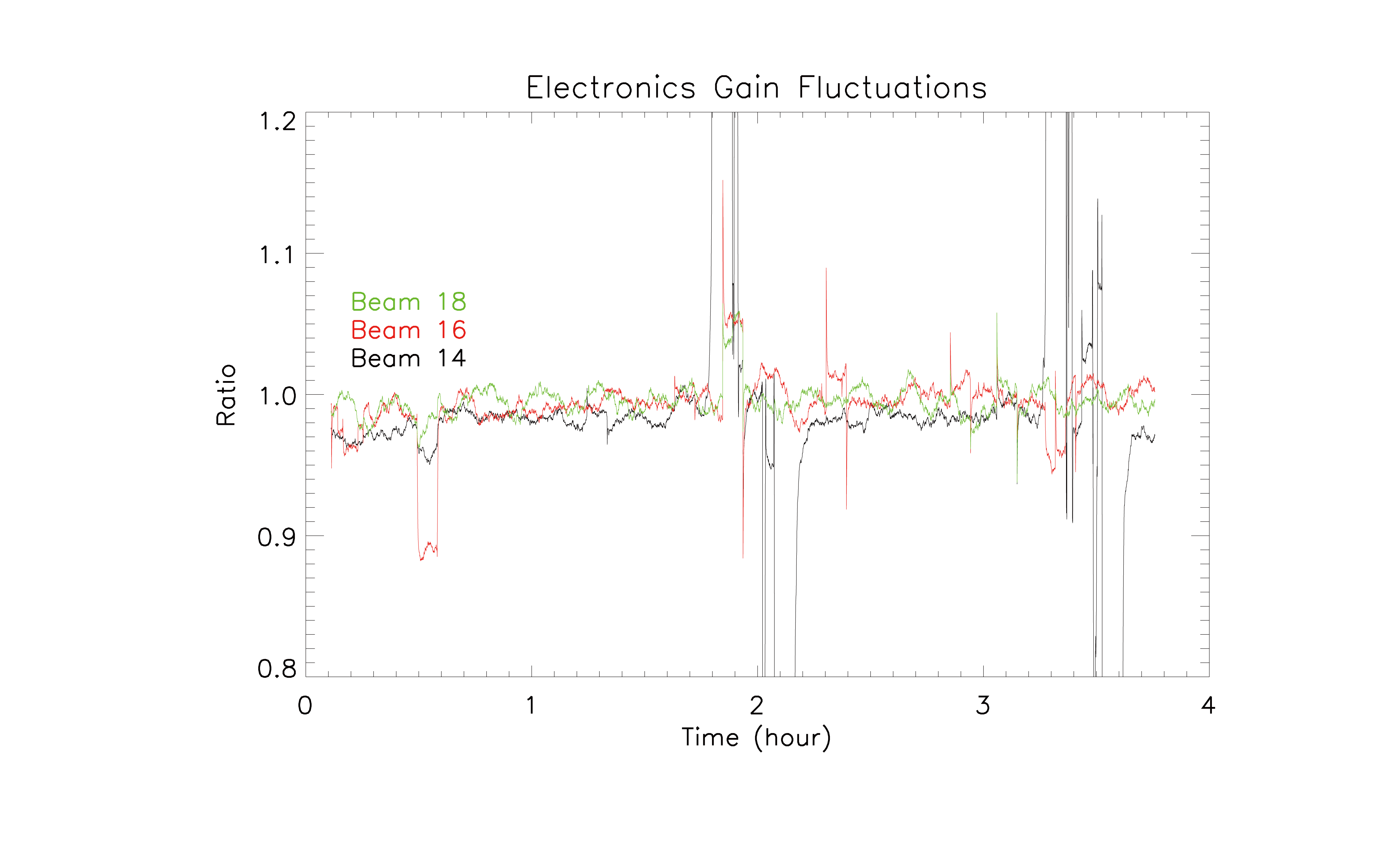
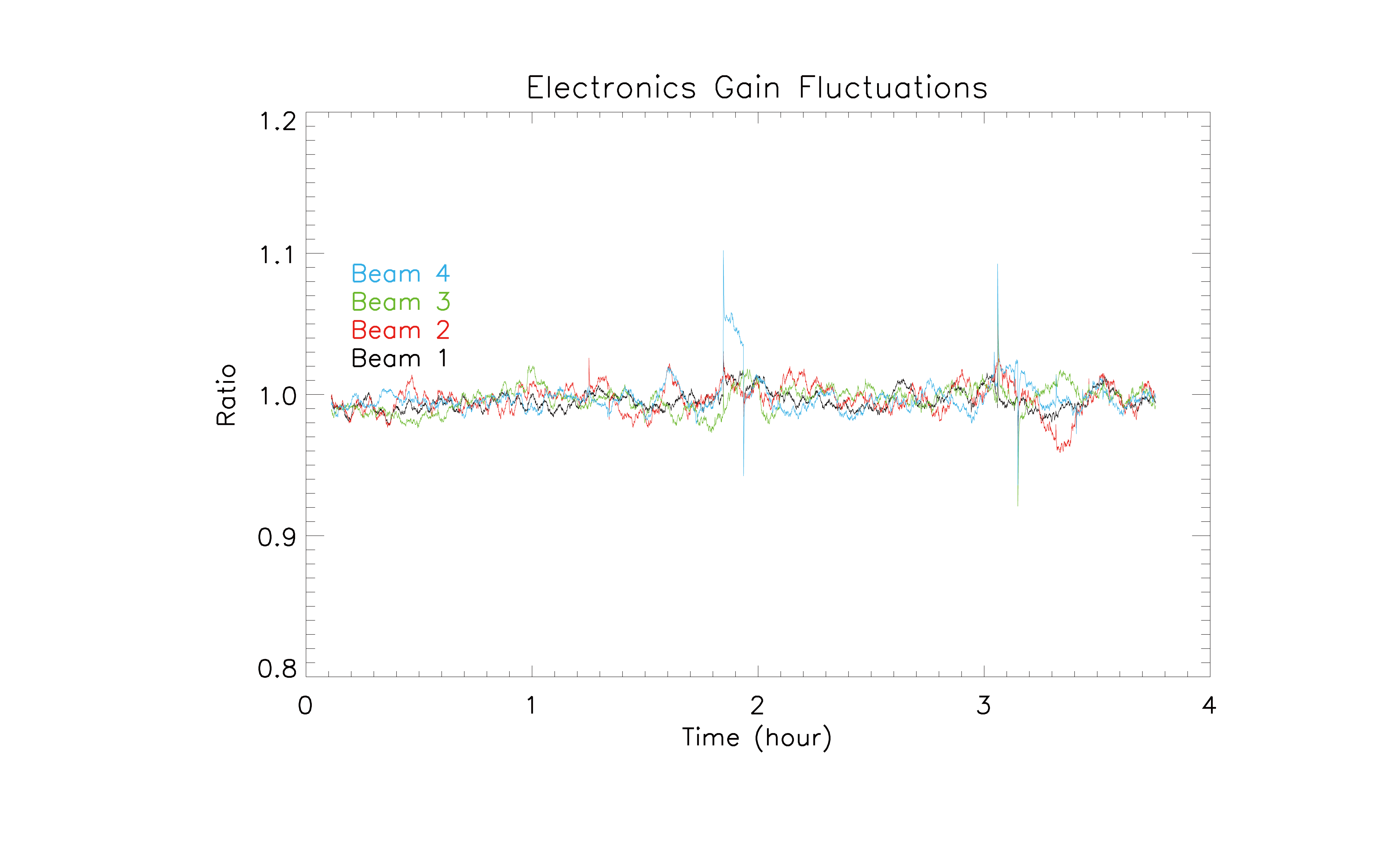
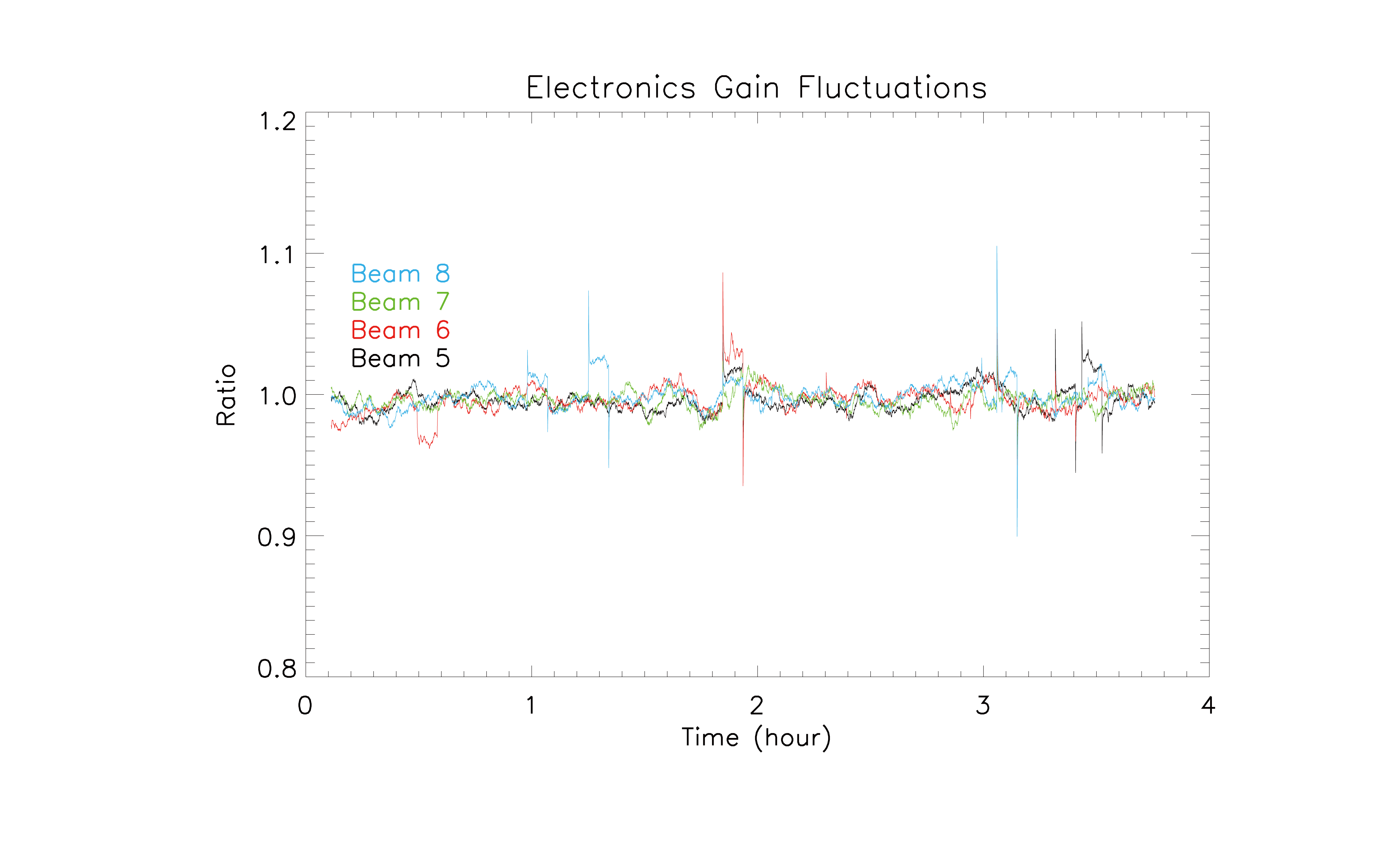
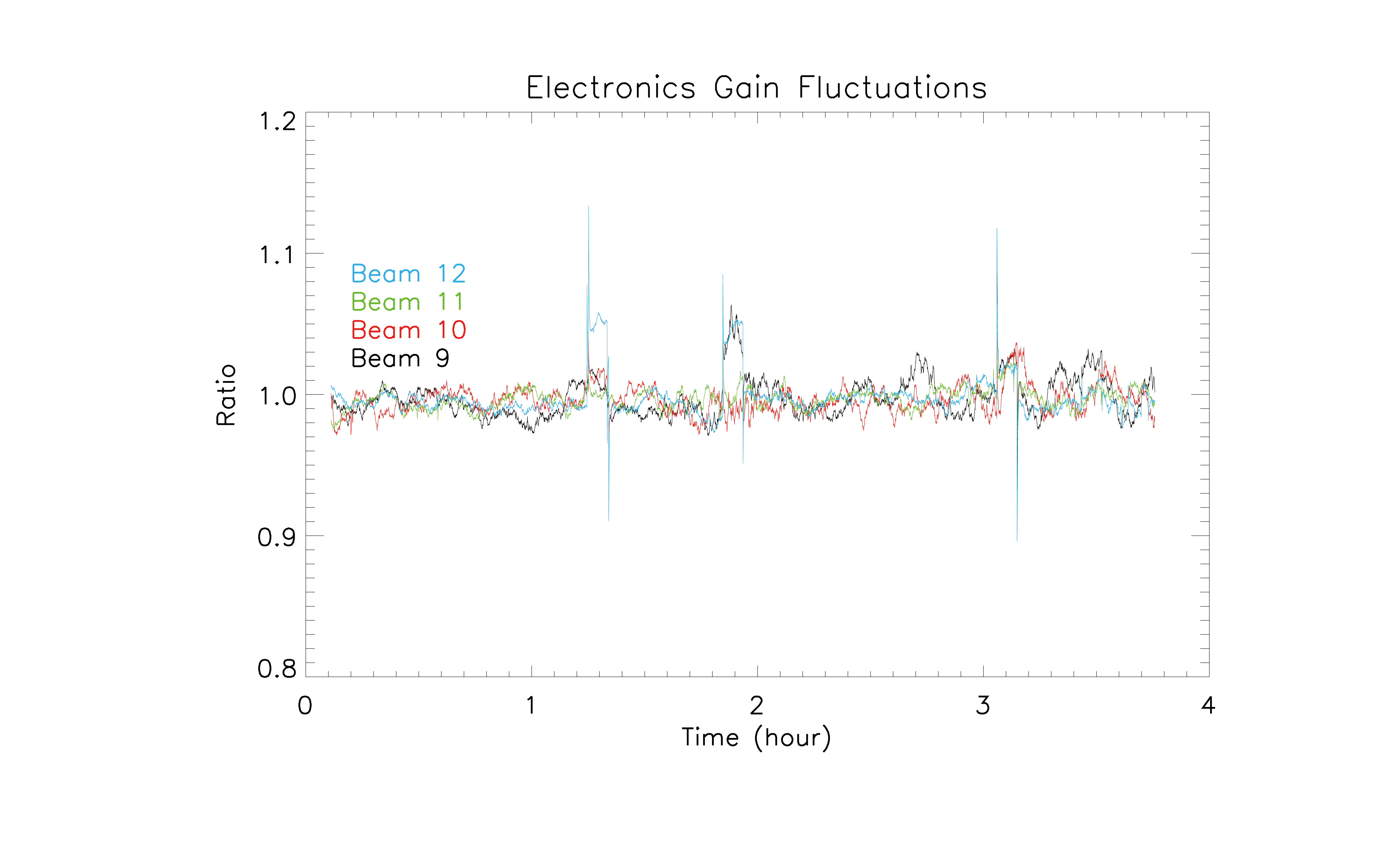
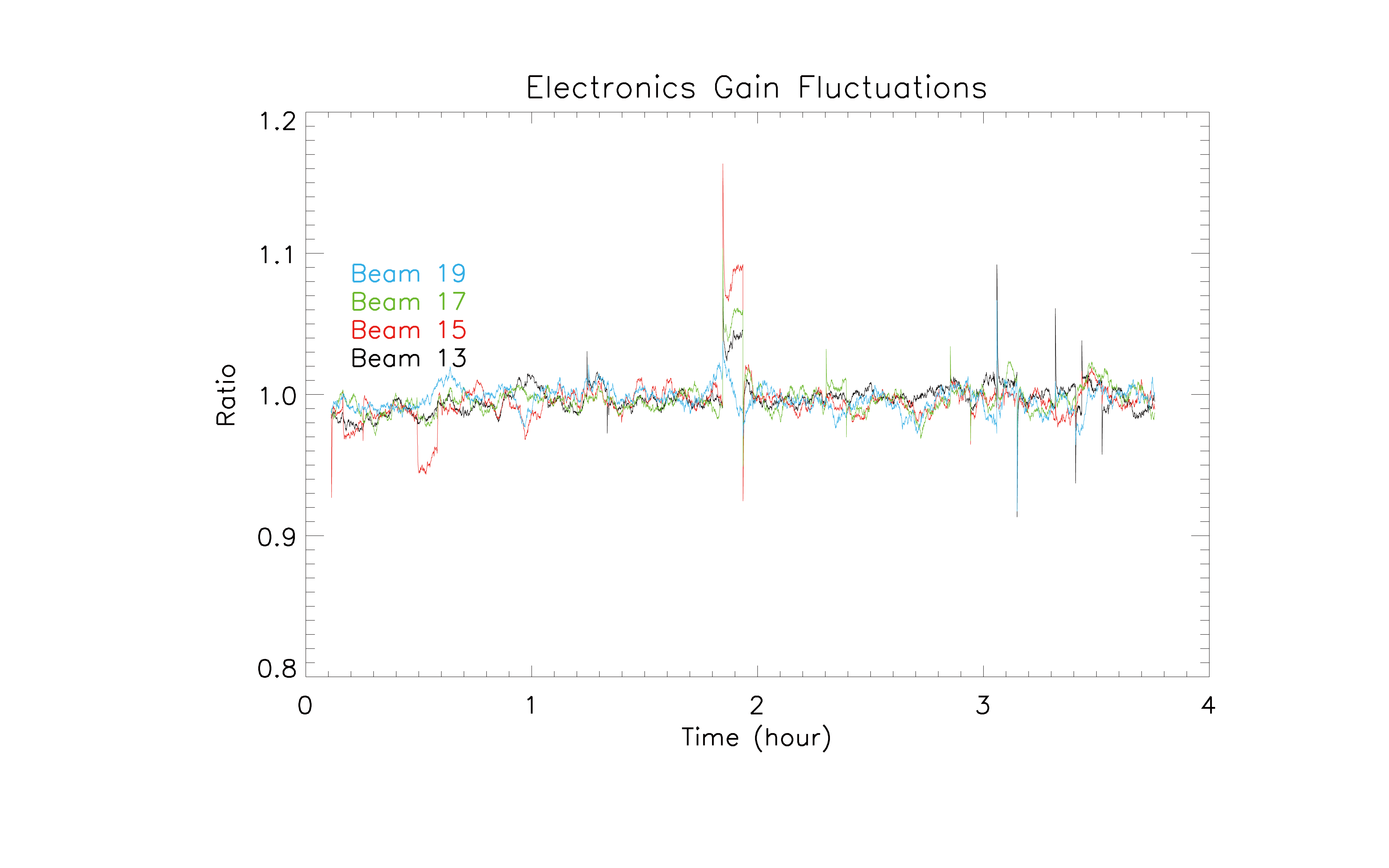
Figure 3 shows the electronics gain fluctuations of the system over several hours. This was done assuming that the noise diode temperature is absolutely constant. It shows that the electronics gain fluctuations within the FAST 19-beam receiver/backend signal path are typically on the order of a few percent over timescales of a few minutes. This implies that science projects for whom flux calibration is important should fire the noise diode at least every few minutes in order to account for typical electronics gain fluctuations. The larger fluctuations in Figure 3 are caused by RFI leaking into the signal path during the hot load measurements, and instability in the low noise amplifiers. The electronics gain fluctuations of the rest beams are presented in the Figure 27.


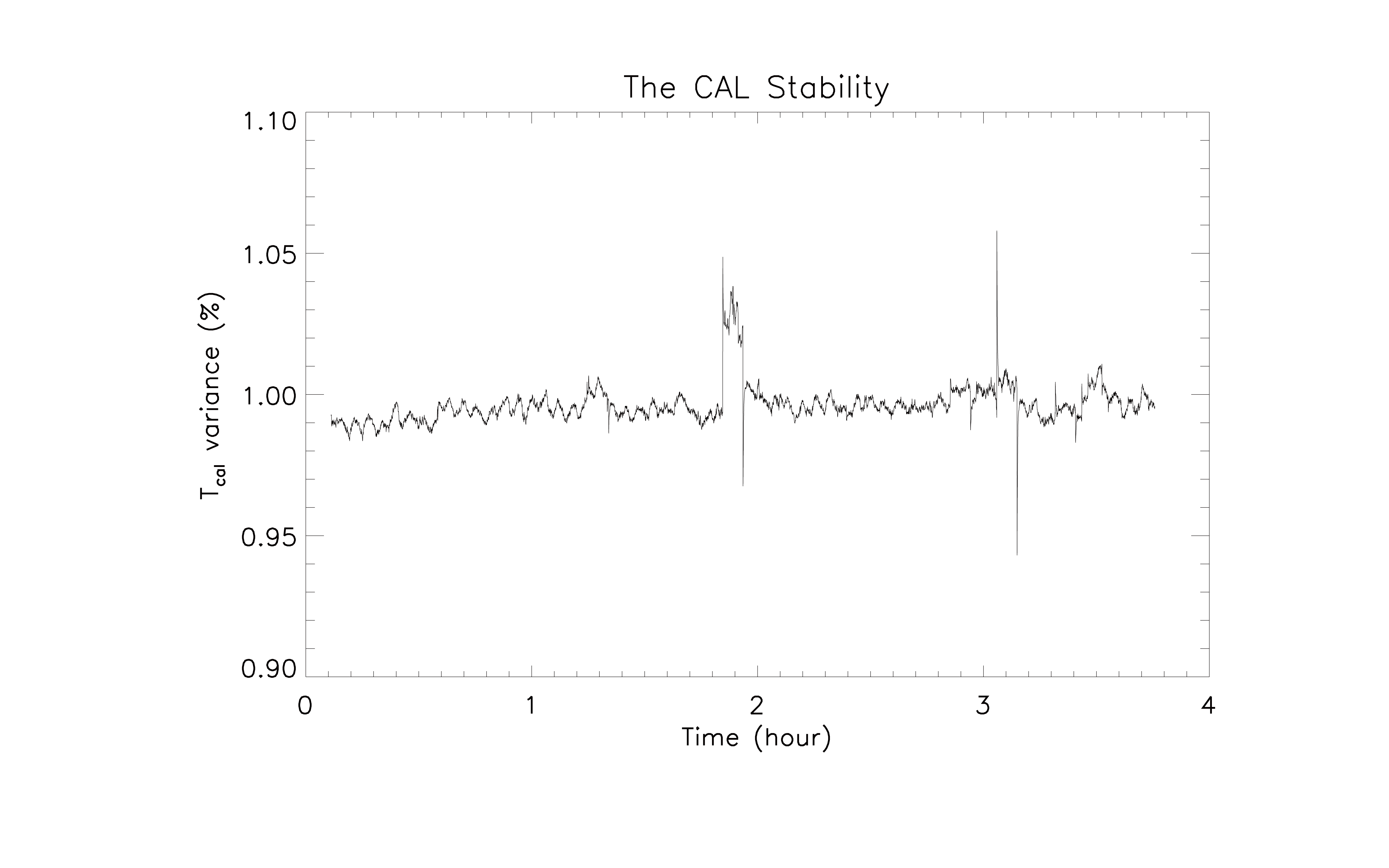
The electronics gain fluctuations in Figure 3 are mostly uncorrelated between the different beams. By taking a median value of all 19 beams, we can produce Figure 4 which yields an upper limit on the temperature fluctuations in the noise diode. While laboratory measurements of the noise diode itself yielded temperature fluctuations on the order of 0.1 over several hours, we see that once placed within the full signal path we get an upper limit of 1, implying that it is likely impossible to obtain accurate flux calibration better than 1. Considering FAST’s pointing accuracy, and beam size the best flux calibration for a point source is approximately 2, meaning that the noise diode is certainly operating within our tolerance limits. This lower limit is estimated by looking at the shape of the beam response function at 1420MHz within the pointing uncertainty limits. The effect is weaker at longer wavelengths where the pointing uncertainty is smaller compared to the beam size.
II.2. Beam Properties and Pointing Accuracy
To measure the properties of FAST’s 19-beam receiver, one method is to directly make mapping observations toward radio sources on the sky. The raster scan (or raster scanning) observation mode has been realized for FAST, which is used to map radio sources and measure the 19-beam properties.
II.2.1 Observations
From November 28 to December 29, 2018, mapping observation have been conducted toward 3C380, 1902+319, 1859+129, 3C454.3, and 2023+318, etc. In the observations, a sky area centering on the target source and covering is mapped by a raster scan along the RA or Dec direction with the 19-beam receiver. An example of the telescope track for a raster scan along Dec is given in Fig. 5. The scan velocity is 15′/min. The separation between two sub-scans is 1′, which satisfies Nyquist sampling. A total of 100 minutes is needed to acquire such a map. Observational data are simultaneously recorded with the pulsar mode, the narrow-band spectral-line mode, and also the wide-band spectral-line mode. The number of channels is 4096 for the pulsar backend and 65536 for the spectral-line backend (wideband mode), corresponding to a frequency coverage from 1000 1500 MHz, which is somewhat broader than the designed bandwidth of the 19-beam receiver (1050 1450 MHz). The sampling time, i.e., the integration time for raw data, is set to 196.608s for the pulsar mode and 1.00663296s for the spectral-line modes. The intensity for each of the 19 beams is calibrated by the periodic injection of a high-intensity noise signal (10 K, see Sect. II.1) with a period of 0.2s.

II.2.2 Data processing procedure
A standard pipeline for processing the mapping data of the 19-beam receiver is still under development. In the following analysis the mapping data is processed using IDL. The data recorded by the pulsar backend are adopted, which have dual linear polarizations (XX and YY) and a relatively high time-resolution. We first compress the data raw data in the time dimension to have an identical time-resolution with the periodic injected noise. The antenna temperature for each of the polarization is then converted from the raw counts by using the noise diode calibrator. The observed intensity (XX or YY, in K) corresponding to a frequency can be extracted from the spectra after a removing of the radio frequency interference (RFI). Together with the data recording time given by the backend, one series of pairs of can be obtained. During the raster scan observation, the phase center of the feed is measured by a real-time measurement system (see Jiang et al. 2019 for a detail), which can be converted to the telescope pointing of the central beam (M01) in the horizontal coordinate system (alt, az). The telescope pointing in the equatorial coordinates (ra, dec in J2000) are then calculated from the horizontal coordinates alt and az after considering the precession, nutation, aberration and also the refraction effect of the atmosphere. With the time information given by the measurement system, we can derive another series of pairs of . By cross-matching time between the two series of flow data, a data-cube with information of RA, Dec and intensity is derived. Then the data-cube can be regridded to construct the intensity map.
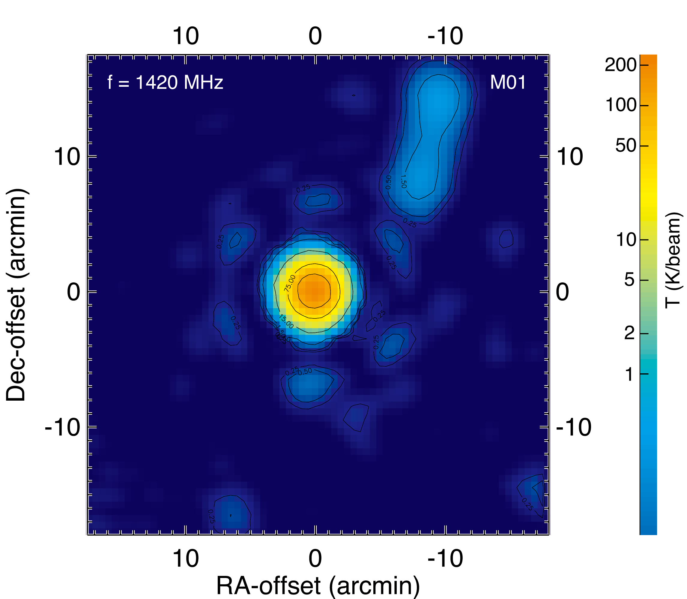
An example of a total intensity map is given in Fig. 5. The continuum background is calculated and removed to show the sidelobes and the weak field sources more clearly in the plots of logarithmic-scale. We compare it with the continuum map of the same sky area obtained by the NRAO/VLA Sky Survey (NVSS) 11 1 https://www.cv.nrao.edu/nvss/postage.shtml at 1.4 GHz, and found that the detected positions of four weak radio sources near RA- and Dec-offsets of (,+15′), (8′,+8′), (6.5′, 16.5′), and (17′,15′) are consistent. Then, the background radio sources are fitted by 2-D Gaussian models and removed. Similar procedure of data processing is made to the mapping data of other beams, and examples of the results are given in Fig. 6. The patterns of beam response shown in Fig. 6 are smilar to the radiation patterns given by simulations (Smith et al. 2016). According to the angular distance of the beam center to that of the central beam M01, , the rest 18 elements of the 19-beam receiver are distributed in three concentric ring-shaped area (see Fig. 7): 1st-ring) M02-M07, with arcmin; 2nd-ring) M09, M11, M13, M15, M17, M19, with arcmin; 3rd-ring) M08, M10, M12, M14, M16, M18, with arcmin. As the increase of , the sidelobes become more and more significant. The morphology of the sidelobes and their angular distances to the beam center depend on the observation frequency. Other notable features are the noncircular morphology and coma of the main beam, which are negligible for the central beam, but seem to become more and more significant as the increase of for the outer beams.

| (2018-12-07) | (2018-12-08) | (2018-12-16) | (2018-12-17) | Mean values | ||||||
| Scan Direction | (Along RA) | (Along Dec) | (Along RA) | (Along Dec) | ||||||
| Beam No. | (′) | (′) | (′) | (′) | (′) | (′) | (′) | (′) | (′) | (′) |
| M01 | 0.00 | 0.00 | 0.02 | 0.01 | 0.06 | 0.05 | 0.06 | 0.02 | 0.04 | 0.02 |
| M02 | 5.81 | 0.03 | 5.81 | 0.03 | 5.69 | 0.05 | 5.73 | 0.04 | 5.76 | 0.01 |
| M03 | 2.89 | 4.97 | 2.94 | 4.93 | 2.81 | 5.06 | 2.83 | 4.99 | 2.86 | 4.98 |
| M04 | 2.84 | 4.99 | 2.81 | 5.00 | 2.95 | 5.03 | 2.95 | 5.02 | 2.89 | 5.01 |
| M05 | 5.75 | 0.03 | 5.74 | 0.01 | 5.82 | 0.04 | 5.80 | 0.01 | 5.78 | 0.02 |
| M06 | 2.90 | 5.00 | 2.91 | 5.00 | 2.92 | 4.94 | 2.94 | 4.97 | 2.92 | 4.98 |
| M07 | 2.89 | 5.01 | 2.85 | 5.03 | 2.83 | 4.90 | 2.83 | 4.95 | 2.85 | 4.97 |
| M08 | 11.58 | 0.01 | 11.60 | 0.05 | 11.49 | 0.06 | 11.53 | 0.07 | 11.55 | 0.02 |
| M09 | 8.67 | 4.96 | 8.74 | 4.93 | 8.56 | 5.07 | 8.64 | 5.06 | 8.65 | 5.01 |
| M10 | 5.81 | 9.99 | 5.89 | 9.94 | 5.69 | 10.10 | 5.70 | 10.04 | 5.78 | 10.02 |
| M11 | 0.08 | 9.99 | 0.13 | 9.96 | 0.09 | 10.05 | 0.10 | 10.06 | 0.00 | 10.04 |
| M12 | 5.69 | 10.06 | 5.65 | 10.10 | 5.90 | 10.07 | 5.90 | 10.07 | 5.78 | 10.07 |
| M13 | 8.57 | 5.07 | 8.60 | 5.05 | 8.75 | 5.05 | 8.74 | 5.04 | 8.67 | 5.05 |
| M14 | — | — | 11.58 | 0.05 | — | — | 11.64 | 0.00 | 11.61 | 0.02 |
| M15 | 8.67 | 4.93 | 8.69 | 5.00 | 8.67 | 4.96 | 8.72 | 4.99 | 8.68 | 4.99 |
| M16 | 5.81 | 10.01 | 5.82 | 10.05 | 5.81 | 10.00 | 5.85 | 10.02 | 5.83 | 10.02 |
| M17 | 0.02 | 10.01 | 0.02 | 10.03 | 0.01 | 9.95 | 0.07 | 9.99 | 0.03 | 10.00 |
| M18 | 5.79 | 10.04 | 5.77 | 10.06 | 5.74 | 9.94 | 5.73 | 9.96 | 5.76 | 10.00 |
| M19 | 8.67 | 5.01 | 8.66 | 5.07 | 8.58 | 4.92 | 8.60 | 4.94 | 8.63 | 4.98 |
To fit the main-beam power pattern with consideration of elliptcity and coma, and determine the combined response of the 19-element multi-beam receiver, we follow the definition of a ’skew Gaussian’ given by Heiles et al. (2004). Nine parameters for the -th beam are the peak intensity , beam center and , the average beamwidth , beam ellipticity , beam orientation , coma with orientation , and a factor . For the central beam M01, and , are the pointing errors of FAST in RA and Dec, respectively. For other beams, the fitting parameter and are taken as the angular offsets relative to the true center of beam M01. For each beam, the main-beam power pattern is parameterized in the polar coordinates (, ) as:
| (1) |
where , . Here, is the angular distance of the position to the true beam center, is the position angle in the equatorial coordinates (RA, Dec in J2000), and defined to be zero along the positive RA-offset axis and increases towards positive Dec-offset axis. Follow Heiles et al. (2004), we also take as a constant parameter 0.75 during the fit. Together with the term min, they are used to prevent the coma term from unduly distorting the beam far from the beam center (Heiles et al. 2004). The MPFIT package22 2 http://www.physics.wisc.edu/ craigm/idl/fitting.html is adopted to make the minimization. In the following, we give a general discussion about the combined beam response, the beamwidth and also the pointing errors of FAST, obtained by fitting the observed total intensity (XX+YY) maps.

II.2.3 The Convolved Beam Pattern of the 19-beam Receiver
To measure the beam properties, we analyzed the mapping data toward 3C454.3, which is the strongest source at 1.4 GHz among the observed targets (1902+319, 1859+129, 3C454.3, and 2023+318, etc) by FAST. Raster scan covering a sky area of were made four times along RA or Dec directions. The fitted parameters of the beam center for each of the 19 beams is given in Table 1. With the fitted beam center, we combine the intensity distribution maps derived by each of the 19 beams to give a composite response of the 19-beam receiver as shown in Fig. 7. The observed layout of the 19-beam receiver is consistent with the schematic diagram given by Dunning et al. (2017) and Li et al. (2018). Around the main beams, the responses of first sidelobes for the 12 outer beams (M08-M19) are also visible in the logarithmic-scale plot. Similar results were obtained by analyzing the observation data toward other sources, e.g., 3C380, 2023+318.
II.2.4 Beamwidth
| Beam No. | Frequency (MHz) | ||||||||||||
| 1060 | 1080 | 1100 | 1120 | 1140 | 1300 | 1320 | 1340 | 1360 | 1380 | 1400 | 1420 | 1440 | |
| M01 | 3.44′ | 3.37′ | 3.31′ | 3.29′ | 3.29′ | 3.01′ | 2.98′ | 2.93′ | 2.89′ | 2.85′ | 2.82′ | 2.82′ | 2.82′ |
| M02 | 3.44′ | 3.37′ | 3.31′ | 3.33′ | 3.33′ | 3.04′ | 3.00′ | 2.96′ | 2.92′ | 2.88′ | 2.85′ | 2.85′ | 2.84′ |
| M03 | 3.44′ | 3.38′ | 3.30′ | 3.33′ | 3.32′ | 3.03′ | 3.00′ | 2.95′ | 2.91′ | 2.87′ | 2.84′ | 2.84′ | 2.83′ |
| M04 | 3.44′ | 3.38′ | 3.31′ | 3.34′ | 3.32′ | 3.05′ | 3.01′ | 2.97′ | 2.93′ | 2.90′ | 2.86′ | 2.86′ | 2.85′ |
| M05 | 3.43′ | 3.36′ | 3.29′ | 3.31′ | 3.32′ | 3.03′ | 2.99′ | 2.95′ | 2.91′ | 2.87′ | 2.83′ | 2.83′ | 2.82′ |
| M06 | 3.44′ | 3.39′ | 3.31′ | 3.34′ | 3.34′ | 3.07′ | 3.03′ | 3.01′ | 3.01′ | 2.99′ | 2.95′ | 2.94′ | 2.99′ |
| M07 | 3.45′ | 3.39′ | 3.31′ | 3.33′ | 3.34′ | 3.02′ | 2.99′ | 2.95′ | 2.92′ | 2.88′ | 2.86′ | 2.86′ | 2.86′ |
| M08 | 3.46′ | 3.42′ | 3.38′ | 3.35′ | 3.34′ | 3.04′ | 3.02′ | 2.98′ | 2.95′ | 2.92′ | 2.90′ | 2.88′ | 2.86′ |
| M09 | 3.48′ | 3.41′ | 3.36′ | 3.33′ | 3.30′ | 3.04′ | 3.01′ | 2.97′ | 2.94′ | 2.91′ | 2.88′ | 2.88′ | 2.86′ |
| M10 | 3.52′ | 3.46′ | 3.40′ | 3.38′ | 3.35′ | 3.08′ | 3.05′ | 3.03′ | 3.00′ | 2.97′ | 2.95′ | 2.94′ | 2.92′ |
| M11 | 3.49′ | 3.43′ | 3.38′ | 3.37′ | 3.34′ | 3.05′ | 3.02′ | 3.00′ | 2.97′ | 2.94′ | 2.92′ | 2.91′ | 2.90′ |
| M12 | 3.49′ | 3.44′ | 3.39′ | 3.37′ | 3.34′ | 3.07′ | 3.05′ | 3.03′ | 3.00′ | 2.97′ | 2.95′ | 2.94′ | 2.90′ |
| M13 | 3.48′ | 3.41′ | 3.34′ | 3.33′ | 3.32′ | 3.04′ | 3.01′ | 2.98′ | 2.95′ | 2.93′ | 2.91′ | 2.91′ | 2.89′ |
| M14 | 3.53′ | 3.48′ | 3.43′ | 3.41′ | 3.38′ | 3.10′ | 3.07′ | 3.04′ | 3.01′ | 2.98′ | 2.95′ | 2.94′ | 2.92′ |
| M15 | 3.49′ | 3.42′ | 3.36′ | 3.36′ | 3.36′ | 3.06′ | 3.01′ | 2.98′ | 2.94′ | 2.91′ | 2.89′ | 2.88′ | 2.86′ |
| M16 | 3.51′ | 3.46′ | 3.41′ | 3.39′ | 3.34′ | 3.10′ | 3.07′ | 3.05′ | 3.02′ | 2.99′ | 2.97′ | 2.95′ | 2.93′ |
| M17 | 3.49′ | 3.42′ | 3.35′ | 3.34′ | 3.33′ | 3.02′ | 3.00′ | 2.99′ | 2.97′ | 2.94′ | 2.92′ | 2.92′ | 2.91′ |
| M18 | 3.55′ | 3.51′ | 3.37′ | 3.33′ | 3.29′ | 3.05′ | 3.04′ | 3.00′ | 2.98′ | 2.96′ | 2.95′ | 2.94′ | 2.93′ |
| M19 | 3.42′ | 3.41′ | 3.36′ | 3.33′ | 3.34′ | 3.03′ | 3.00′ | 2.98′ | 2.95′ | 2.93′ | 2.91′ | 2.90′ | 2.89′ |
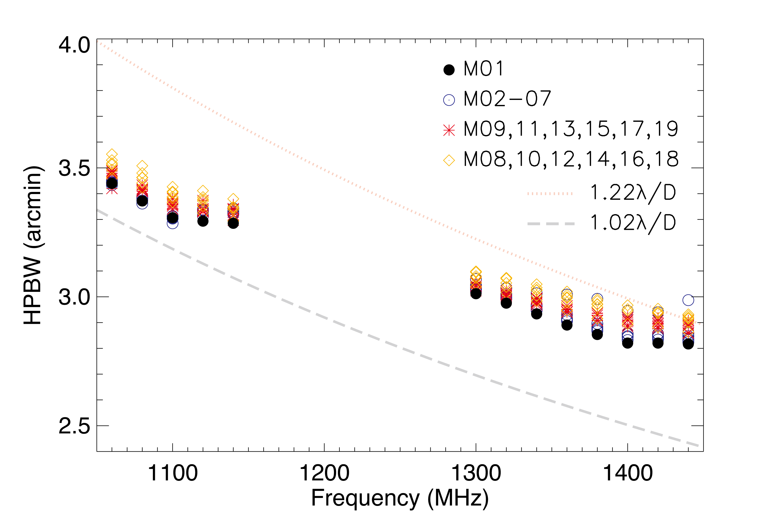
The half-power beamwidth (HPBW) is related to the average beamwidth by HPBW , here, is derived by fitting the total intensity distribution maps with a ’skew Gaussian’ model as shown in Eq. 1. The HPBW as a function of the observation frequency for the 19 beams are given in Fig. 8. In comparison to the central beam, the outer beams tend to have larger beamwidths, with a difference no more than 0.2 arcmin. The HPBW decreases with the increase of frequency. As discussed in Jiang et al. (2019), the theoretical HPBW of a telescope with diameter is HPBW for a uniformly illuminated aperture and HPBW for a cosine-tapered illuminated aperture. Here, a diameter of m is assumed. As shown in Fig. 8, the fitted beamwidths of the 19-beam receiver fall within the two theoretical curves of HPBW verseus frequency, but with a less steep slope than that of a standard proportionality.

II.2.5 Pointing errors
As discussed in Jiang et al. (2019), the analysis of pointing errors can be used to evaluate the pointing accuracy, improve the pointing of the telescope, and also guide the error analysis of observations. Systematic observations have been made to measure the pointing errors of FAST by raster scan observations. As we only care about the pointing errors of the central beam M01, the mapping area toward a target source is set to . About 7 minutes is needed to acquire such a map with subscan separation of 1′. The target sources are selected from the catalogue of pointing calibrators given by Condon & Yin (2001), which contains 3399 strong and compact radio sources with accurate positions from the NVSS, and uniformly covering the sky north of (J2000). The dataset used in the analysis are observed from February 16 to March 15, 2019, which include 126 raster scan observations along RA or Dec directions. As shown in Fig. 9, the observed pointing calibrators distribute widely in the sky coverage of FAST with full gain (zenith angle ).
The observation data are processed in a similar procedure as described in Sect.2.2.2. To fit the pointing errors in RA and Dec directions, a 2-D Gaussian model is adopted, which is good enough as the central beam do not present significant beam ellipticity and coma feature (Fig. 5 and Fig. 6). The pointing errors are typically smaller than 16′′ as shown in Fig. 10. The rms of pointing errors is 7.9′′, which is less than one-tenth of the beamwidth near 1450 MHz (beamwidth1450/10 2.8′/10 = 16.8′′).

II.3. Aperture Efficiency and System Temperature
Aperture efficiency () and system temperature (Tsys) are two basic parameters of FAST. Both of them are expected to vary as a function of zenith angle () and frequency. The 19 beams are divided into 4 categories according to separation to the central beam. The 4 categories are : 1) Beam 1; 2) Beam 2, 3, 4, 5, 6, and 7; 3) Beam 8, 10, 12, 14, 16, and 18; 4) Beam 9, 11, 13, 15, 17 and 19. Though the performance of aperture efficiency and system temperature in each category is expected to be same, asymmetry of the receiver platform may lead to deviation. Thus we obtained the measurements toward all 19 beams.
The aperture efficiency curve was obtained by repeating observations of the calibrator 3C286 and its off position at different zenith angles. The position switch mode that is introduced in section IV was adopted. This mode provides quick switch between ON and OFF source position. The separation between ON and OFF position was selected to allow for measuring aperture efficiency curve of two beams (e.g, Beam 1 and 19) simultaneously, which increases measurement efficiency.
Observations of Beam 1, 2, 8, and 19 were taken during August 7, 2019 and August 24, 2019. To make it clear, we take the aperture efficiency measurement of Beam 1 and 19 as an example. At first, the telescope tracked the calibrator 3C286 with Beam 1 (source ON for Beam 1, source OFF position for Beam 19) for 90 s, and then switched to the sky position with offset of (-8.85′, -5.11′). At this position, the calibrator 3C286 was OFF for Beam 1 but lay in Beam 19. After tracking for 90s, the telescope switched back to track 3C286 with Beam 1. A cycle consists of one ON and one OFF phase for each beam. A total of 90 cycles were taken during available tracking time of 6 hours of 3C286. Supplementary measurements of the aperture efficiency curve for the rest 15 beams were taken by tracking 3C286 during December 19, 2019 and December 25, 2019. During these observations, the total tracking time in a cycle was reduced into 60 s, including 30 s for both source on and source off. A total of 85 cycles and 3 hours were taken for measurement of both two beams.
The system temperature curve of 19 beams was obtained by continuously tracking a clean sky position (=23h30m0s.0, =25∘39′10.6") from rise to set on September 14, 2019.
In the above measurements, spectral backend with sampling time of 1.00663296 s and channel width of 7.62939 kHz was adopted to record the data. The high noise signal ( K) was injected at a synchronized period of 2.01326592 s. The duration time of cal on and cal off is 1.00663296 s. During calculation, channel width of the data were smoothed to 1 MHz. The aperture efficiency was derived for each observation cycle while the system temperature was derived for each sampling time.
II.3.1 Aperture efficiency
Based on absolute measurement of noise dipole in Section II.1, the observed data were calibrated into antenna temperature in K . The antenna temperature of 3C286, was derived by the difference between source ON and source OFF data for each beam.
3C286 is a stable flux calibrator. The frequency dependency of the spectral flux density of 3C286 could be fitted with a polynomial function (Perley & Butler 2017),
| (2) |
where S and are the spectral flux density in Jy and the frequency respectively. We adopted the value of , , and that is valid for 3C286 at frequency range of [0.05-50] GHz (Perley & Butler 2017).
Measured gain () of FAST is expressed as , in which is effective illumination area. In observation, is calculated by ratio between antenna temperature and flux density, . The prefect gain of FAST is for single polarization, in which and are geometric illumination area and Boltzmann constant respectively. The geometric illumination area with diameter of 300 m leads to = 25.6 K/Jy for FAST.
The aperture efficiency of FAST is derived by,
| (3) |
For the FAST system, is contributed by 6 main components:
- 1.
, the reflection efficiency of main reflector. It is described by equation, , in which and are root mean square (RMS) of the surface error and observational wavelength, respectively. The RMS of the surface error is contributed by controlling accuracy of panels, which is mm at 21 cm (Jiang et al. 2019). This results in of 91%.
- 2.
, the efficiency when the shielding of the feed cabin is considered. The diameter of feed cabin of m leads to value of 99.9%.
- 3.
, spillover efficiency.
- 4.
, illumination efficiency of the feed. It equals 76% when a -13 dB Gaussian illumination is adopted (Jiang et al. 2019).
- 5.
, efficiency of other aspects including the offset of the feed phase, matching loss of feed.
- 6.
, the percent of effective surface area compared to a 300-m diameter paraboloid. The value is 1 when is less than 26.4∘. When is greater than 26.4∘, the reflection area decreases. would decrease and reach 2/3 when .
The aperture efficiency is a synthetical result of above effects and is described by the following equation,
| (4) |
The value of ,,,,and are almost constant. The value of is mainly determined by . As shown in Fig. 11, the value at all frequency would keep almost constant when is less than 26.4∘ and decreases linearly when >26.4∘. This is consistent with the fact that FAST would lose part of reflection panels when >26.4∘.
We fitted variation of as a function of at specific frequency with two linear equations. The formula is shown as follows,
| (5) |
In which satisfies the equation . The fitting result of parameter , and for different frequencies are shown in Table 3. As an example, the fitting results of for Beam 1, 2, 8 and 19 are shown in Fig. 11. The fitting results of rest 15 beams are shown in Fig. 28.
The gain of FAST could be expressed with , in which = 25.6 K/Jy. Flux density (in unit of Jy) of point source is converted from antenna temperature by dividing the gain value. The averaged gain values of 19 beams within ZA of 26.4 ∘ are shown in Table 5. The Beam 16 has smallest gain value among 19 beams. The gain ratio of Beam 16 compared to Beam 1 reaches at 1400 and 1450 MHz.
II.3.2 System Temperature
Observation of sky position (=23h30m0s.0, =25∘39′10.6") allows us to measure system temperature from zenith angle of 40∘ to nearly . The data were calibrated into antenna temperature in K with noise curve. For a single dish telescope at L band, Tsys consists four main sources (Campbell et al. 2002):
- 1.
Noise contribution from receiver, . For 19 beam receiver of FAST, it is measured as 7-9 K, including 4 K from low noise amplifier (LAN) (see section 4.1.1 in Jiang et al. 2019 for details).
- 2.
Continuum brightness temperature of the sky, . This includes 2.73 K from cosmic microwave background (CMB) and non-thermal emission from the Milky Way. The value of at 1.4 GHz is K toward position (=23h30m0s.0, =25∘39′10.6") (CHIPASS survey; Calabretta et al. 2014).
- 3.
Emission from the Earth’s atmosphere . This value should be in a few K.
- 4.
Radiation from the surrounding terrain, . This contribution originates from side lobe of FAST. Unlike other single dish with fixed surface and horn, the illumination area of horn varies for different zenith angle, leading to different value of .
System temperature are synthetical result of the above components.
| (6) |
The variation of system temperature as a function of zenith angle could be fitted with the following formula,
| (7) |
which is valid for . The value of , , and in different frequencies are shown in Table 4. An example of fitting curve is shown in Fig. 12. The results for the rest beams are shown in Fig. 29.
A significant feature in the profile is that the value of most beams reaches its minimum at ZA range of [10∘,15∘]. When ZA is smaller than 10∘, the value would increase by a maximum value of 1 K. Though central hole of spherical surface was shielded with metal mesh during observations, the leakage of ground emission ( K) from the central hole goes into the main beam and contributes increase when ZA is less than 10∘. When ZA gets larger than 15∘, the value increases by 5-7 K, which arises from emission of nearby mountain through sidelobe.
II.3.3 Discussion
The observations lie in range of [4.9,40] deg for curve. The fitting results are expected to be valid for range of [0,40] degree for the following reasons. When , there is no loss of panel. In this case, should keep almost constant as shown in the fitting curves.
| Beam | Paras | Freq (MHz) | ||||||||
|---|---|---|---|---|---|---|---|---|---|---|
| 1050 | 1100 | 1150 | 1200 | 1250 | 1300 | 1350 | 1400 | 1450 | ||
| M01 | a/1e-4 | 3.31 2.23 | 2.54 1.85 | 0.34 1.83 | 5.03 2.03 | 4.94 2.02 | 9.83 1.85 | 8.50 1.93 | 7.87 1.95 | 10.64 1.90 |
| M01 | b/1e-1 | 6.19 0.04 | 6.32 0.03 | 6.43 0.03 | 6.22 0.03 | 6.22 0.03 | 6.08 0.03 | 6.12 0.03 | 6.14 0.03 | 5.98 0.03 |
| M01 | c/1e-2 | -1.58 0.02 | -1.61 0.03 | -1.37 0.04 | -1.40 0.04 | -1.42 0.03 | -1.38 0.03 | -1.40 0.02 | -1.34 0.02 | -1.26 0.02 |
| M02 | a/1e-4 | 9.46 3.53 | 6.28 3.09 | 9.01 3.14 | 12.13 3.12 | 10.98 3.06 | 11.31 2.16 | 8.71 2.09 | 8.78 2.06 | 13.07 1.98 |
| M02 | b/1e-1 | 5.97 0.06 | 5.97 0.05 | 5.99 0.05 | 5.81 0.05 | 5.81 0.05 | 5.65 0.04 | 5.75 0.03 | 5.75 0.03 | 5.62 0.03 |
| M02 | c/1e-2 | -1.54 0.03 | -1.62 0.03 | -1.46 0.03 | -1.44 0.02 | -1.42 0.02 | -1.29 0.02 | -1.32 0.02 | -1.33 0.02 | -1.21 0.02 |
| M03 | a/1e-4 | 1.79 4.21 | 4.39 3.55 | 2.41 4.46 | 5.95 4.69 | 6.90 3.21 | 7.41 2.60 | 9.99 2.63 | 7.66 2.60 | 10.30 2.72 |
| M03 | b/1e-1 | 6.41 0.07 | 6.24 0.06 | 6.42 0.07 | 6.21 0.07 | 6.17 0.05 | 6.07 0.04 | 5.91 0.04 | 5.99 0.04 | 5.86 0.04 |
| M03 | c/1e-2 | -1.70 0.03 | -1.80 0.03 | -1.56 0.03 | -1.63 0.02 | -1.59 0.02 | -1.56 0.02 | -1.53 0.02 | -1.47 0.02 | -1.35 0.03 |
| M04 | a/1e-4 | 3.57 4.76 | 1.87 4.08 | 3.82 3.93 | 3.90 4.60 | 8.46 4.65 | 4.29 3.22 | 2.75 3.28 | 1.85 3.26 | 5.10 3.20 |
| M04 | b/1e-1 | 6.24 0.08 | 6.15 0.07 | 6.25 0.06 | 6.05 0.08 | 5.98 0.08 | 5.92 0.05 | 5.89 0.05 | 5.89 0.05 | 5.75 0.05 |
| M04 | c/1e-2 | -1.80 0.03 | -1.82 0.03 | -1.65 0.02 | -1.57 0.06 | -1.58 0.02 | -1.42 0.02 | -1.45 0.02 | -1.36 0.02 | -1.24 0.02 |
| M05 | a/1e-4 | -3.97 2.87 | -4.25 2.72 | -4.44 2.72 | -7.54 3.48 | -4.09 4.19 | -5.41 2.35 | -3.33 2.26 | -4.51 2.42 | -4.58 2.53 |
| M05 | b/1e-1 | 6.45 0.05 | 6.48 0.04 | 6.68 0.04 | 6.42 0.06 | 6.39 0.07 | 6.26 0.04 | 6.10 0.04 | 6.17 0.04 | 6.11 0.04 |
| M05 | c/1e-2 | -1.82 0.03 | -1.86 0.03 | -1.72 0.03 | -1.56 0.03 | -1.60 0.03 | -1.53 0.02 | -1.45 0.03 | -1.44 0.03 | -1.30 0.03 |
| M06 | a/1e-4 | 1.69 2.84 | 0.74 2.59 | -0.00 4.17 | 1.06 5.18 | 0.97 3.49 | 0.33 1.82 | 3.11 1.80 | -0.03 1.76 | 1.37 1.76 |
| M06 | b/1e-1 | 6.16 0.04 | 6.22 0.04 | 6.33 0.07 | 6.01 0.08 | 6.04 0.06 | 5.92 0.03 | 5.83 0.03 | 5.89 0.03 | 5.75 0.03 |
| M06 | c/1e-2 | -1.74 0.03 | -1.80 0.03 | -1.60 0.03 | -1.50 0.04 | -1.44 0.03 | -1.33 0.02 | -1.38 0.02 | -1.35 0.02 | -1.22 0.02 |
| M07 | a/1e-4 | 1.71 2.43 | 0.08 2.18 | 0.77 2.41 | 2.03 3.25 | 2.24 3.64 | 3.46 1.82 | 5.46 1.60 | 6.70 1.65 | 6.91 1.49 |
| M07 | b/1e-1 | 6.10 0.04 | 6.04 0.04 | 6.18 0.04 | 5.90 0.05 | 6.02 0.06 | 5.86 0.03 | 5.77 0.03 | 5.73 0.03 | 5.62 0.02 |
| M07 | c/1e-2 | -1.68 0.02 | -1.64 0.02 | -1.52 0.02 | -1.39 0.02 | -1.43 0.02 | -1.32 0.02 | -1.34 0.02 | -1.36 0.02 | -1.22 0.02 |
| M08 | a/1e-4 | 13.91 3.13 | 17.00 2.98 | 14.04 3.81 | 16.81 4.98 | 17.71 2.95 | 17.29 2.75 | 16.95 2.29 | 15.92 2.31 | 17.76 2.43 |
| M08 | b/1e-1 | 5.76 0.05 | 5.75 0.05 | 5.81 0.06 | 5.62 0.08 | 5.54 0.05 | 5.46 0.04 | 5.41 0.04 | 5.34 0.04 | 5.22 0.04 |
| M08 | c/1e-2 | -1.60 0.06 | -1.70 0.05 | -1.52 0.06 | -1.50 0.06 | -1.50 0.05 | -1.47 0.05 | -1.45 0.05 | -1.37 0.05 | -1.28 0.05 |
| M09 | a/1e-4 | -1.26 2.03 | -0.43 1.99 | -2.68 1.94 | 0.12 1.67 | 0.96 1.60 | 1.53 1.53 | 1.09 1.36 | 1.00 1.11 | 0.27 0.91 |
| M09 | b/1e-1 | 5.96 0.03 | 5.95 0.03 | 5.98 0.03 | 5.75 0.03 | 5.77 0.03 | 5.74 0.02 | 5.64 0.02 | 5.57 0.02 | 5.53 0.02 |
| M09 | c/1e-2 | -1.39 0.04 | -1.43 0.03 | -1.28 0.04 | -1.24 0.04 | -1.24 0.03 | -1.18 0.04 | -1.09 0.04 | -1.06 0.03 | -1.01 0.03 |
| M10 | a/1e-4 | 14.36 3.80 | 15.37 3.39 | 15.65 3.78 | 15.20 4.85 | 18.06 2.92 | 17.97 2.67 | 19.34 2.49 | 16.72 2.52 | 18.57 2.65 |
| M10 | b/1e-1 | 6.01 0.06 | 5.98 0.05 | 6.04 0.06 | 5.81 0.08 | 5.86 0.05 | 5.75 0.04 | 5.72 0.04 | 5.69 0.04 | 5.60 0.04 |
| M10 | c/1e-2 | -1.79 0.04 | -1.83 0.04 | -1.74 0.03 | -1.73 0.03 | -1.78 0.03 | -1.74 0.03 | -1.72 0.03 | -1.66 0.03 | -1.58 0.03 |
| M11 | a/1e-4 | 7.68 5.51 | 2.98 4.73 | 4.16 4.57 | 3.38 6.44 | 2.45 4.86 | 4.27 3.39 | 5.99 3.36 | 5.03 3.28 | 8.23 3.05 |
| M11 | b/1e-1 | 5.90 0.09 | 5.94 0.08 | 6.00 0.07 | 5.81 0.10 | 5.80 0.08 | 5.67 0.06 | 5.66 0.05 | 5.61 0.05 | 5.45 0.05 |
| M11 | c/1e-2 | -1.59 0.04 | -1.59 0.03 | -1.55 0.03 | -1.35 0.05 | -1.36 0.03 | -1.31 0.03 | -1.35 0.02 | -1.27 0.02 | -1.18 0.02 |
| M12 | a/1e-4 | -3.00 5.82 | -2.08 4.75 | 1.33 4.29 | 4.98 5.10 | 8.50 4.02 | -0.98 3.17 | 2.94 3.06 | 2.49 2.71 | 2.77 2.60 |
| M12 | b/1e-1 | 6.06 0.09 | 5.96 0.08 | 5.91 0.07 | 5.82 0.08 | 5.76 0.06 | 5.70 0.05 | 5.58 0.05 | 5.53 0.04 | 5.48 0.04 |
| M12 | c/1e-2 | -1.56 0.05 | -1.49 0.04 | -1.45 0.05 | -1.56 0.05 | -1.69 0.03 | -1.35 0.04 | -1.40 0.03 | -1.34 0.03 | -1.27 0.03 |
| M13 | a/1e-4 | -1.33 4.57 | 0.41 4.05 | 2.41 4.07 | -1.35 4.89 | 2.44 3.87 | 2.60 3.22 | 4.14 3.11 | 5.50 2.95 | 5.83 2.77 |
| M13 | b/1e-1 | 6.18 0.08 | 6.12 0.07 | 6.22 0.07 | 6.23 0.08 | 6.04 0.06 | 6.00 0.05 | 5.94 0.05 | 5.85 0.05 | 5.71 0.05 |
| M13 | c/1e-2 | -1.49 0.04 | -1.59 0.03 | -1.53 0.04 | -1.54 0.07 | -1.54 0.03 | -1.57 0.02 | -1.59 0.03 | -1.53 0.03 | -1.44 0.03 |
| M14 | a/1e-4 | 0.35 3.81 | -0.57 3.77 | 4.27 3.61 | 3.01 4.84 | 7.37 4.78 | 2.58 2.61 | 4.43 2.19 | 5.43 2.22 | 5.53 2.19 |
| M14 | b/1e-1 | 5.91 0.06 | 5.98 0.06 | 5.91 0.06 | 5.76 0.08 | 5.73 0.08 | 5.78 0.04 | 5.64 0.04 | 5.59 0.04 | 5.53 0.04 |
| M14 | c/1e-2 | -1.56 0.04 | -1.67 0.04 | -1.65 0.04 | -1.57 0.04 | -1.64 0.03 | -1.68 0.02 | -1.61 0.03 | -1.60 0.04 | -1.51 0.04 |
| M15 | a/1e-4 | 1.33 2.89 | -0.59 2.55 | -3.57 3.01 | 3.71 5.82 | -1.46 2.36 | -2.34 1.73 | -2.80 1.71 | -3.55 1.68 | -2.20 1.64 |
| M15 | b/1e-1 | 5.62 0.05 | 5.78 0.04 | 5.83 0.05 | 5.59 0.09 | 5.68 0.04 | 5.61 0.03 | 5.53 0.03 | 5.50 0.03 | 5.46 0.03 |
| M15 | c/1e-2 | -1.42 0.04 | -1.53 0.03 | -1.34 0.04 | -1.53 0.03 | -1.42 0.03 | -1.32 0.03 | -1.27 0.03 | -1.21 0.03 | -1.13 0.03 |
| M16 | a/1e-4 | 9.81 3.39 | 3.14 3.06 | 0.38 4.28 | 3.85 3.48 | 6.30 2.65 | 5.25 2.13 | 2.32 1.95 | 0.49 1.90 | 1.14 1.83 |
| M16 | b/1e-1 | 5.44 0.06 | 5.52 0.05 | 5.55 0.07 | 5.47 0.06 | 5.29 0.04 | 5.28 0.04 | 5.19 0.03 | 5.17 0.03 | 5.09 0.03 |
| M16 | c/1e-2 | -1.58 0.04 | -1.52 0.03 | -1.46 0.03 | -1.51 0.03 | -1.41 0.02 | -1.36 0.02 | -1.28 0.02 | -1.21 0.02 | -1.14 0.02 |
| M17 | a/1e-4 | -0.89 3.92 | -4.49 3.39 | -3.98 3.71 | -7.57 4.51 | -3.25 2.74 | -0.30 2.47 | -0.80 2.36 | -1.44 2.17 | -0.64 2.08 |
| M17 | b/1e-1 | 5.81 0.06 | 5.83 0.06 | 5.85 0.06 | 5.71 0.07 | 5.65 0.05 | 5.47 0.04 | 5.48 0.04 | 5.41 0.04 | 5.28 0.03 |
| M17 | c/1e-2 | -1.54 0.02 | -1.52 0.02 | -1.41 0.02 | -1.25 0.03 | -1.33 0.02 | -1.22 0.01 | -1.21 0.02 | -1.16 0.01 | -1.08 0.02 |
| M18 | a/1e-4 | -1.88 2.27 | -5.55 2.09 | -5.94 2.11 | -1.53 2.53 | -2.21 3.35 | -0.75 1.52 | -1.19 1.52 | 0.24 1.51 | 0.93 1.53 |
| M18 | b/1e-1 | 5.64 0.04 | 5.68 0.03 | 5.81 0.03 | 5.60 0.04 | 5.57 0.05 | 5.46 0.02 | 5.38 0.02 | 5.38 0.02 | 5.33 0.02 |
| M18 | c/1e-2 | -1.37 0.02 | -1.34 0.02 | -1.34 0.02 | -1.29 0.02 | -1.20 0.02 | -1.13 0.02 | -1.11 0.02 | -1.11 0.02 | -1.05 0.02 |
| M19 | a/1e-4 | 11.82 2.94 | 6.55 2.78 | 5.01 3.51 | 10.73 3.34 | 9.32 2.79 | 8.64 2.51 | 10.22 2.15 | 9.32 2.21 | 11.03 2.24 |
| M19 | b/1e-1 | 5.70 0.05 | 5.88 0.04 | 5.92 0.06 | 5.67 0.05 | 5.69 0.04 | 5.61 0.04 | 5.48 0.03 | 5.43 0.04 | 5.30 0.04 |
| M19 | c/1e-2 | -1.76 0.03 | -1.75 0.03 | -1.59 0.03 | -1.60 0.04 | -1.57 0.03 | -1.50 0.03 | -1.44 0.03 | -1.36 0.03 | -1.25 0.03 |
| Beam | Paras | Freq (MHz) | ||||||||
|---|---|---|---|---|---|---|---|---|---|---|
| 1050 | 1100 | 1150 | 1200 | 1250 | 1300 | 1350 | 1400 | 1450 | ||
| M01 | P0 | 4.94 0.01 | 5.83 0.01 | 4.36 0.01 | 4.24 0.03 | 4.35 0.02 | 3.60 0.01 | 3.10 0.01 | 2.76 0.01 | 2.00 0.01 |
| M01 | P1 | 9.12 0.02 | 8.75 0.03 | 7.53 0.03 | 7.75 0.08 | 6.88 0.04 | 9.88 0.03 | 10.03 0.04 | 10.00 0.04 | 11.93 0.07 |
| M01 | P2 | 26.31 0.01 | 28.14 0.01 | 26.89 0.01 | 27.19 0.02 | 25.54 0.01 | 24.59 0.01 | 23.91 0.00 | 23.47 0.00 | 22.23 0.00 |
| M01 | n | 1.37 0.00 | 1.34 0.00 | 1.26 0.00 | 1.27 0.01 | 1.21 0.00 | 1.41 0.00 | 1.43 0.00 | 1.42 0.00 | 1.53 0.00 |
| M02 | P0 | 4.10 0.00 | 4.53 0.01 | 4.23 0.02 | 4.17 0.05 | 4.08 0.02 | 3.20 0.00 | 2.47 0.00 | 2.29 0.00 | 1.49 0.00 |
| M02 | P1 | 7.68 0.01 | 7.89 0.03 | 6.19 0.03 | 6.32 0.07 | 5.73 0.03 | 8.83 0.02 | 9.36 0.02 | 9.32 0.02 | 11.41 0.06 |
| M02 | P2 | 25.65 0.00 | 26.74 0.01 | 26.63 0.02 | 27.53 0.04 | 25.56 0.02 | 24.14 0.00 | 23.29 0.00 | 23.23 0.00 | 21.87 0.00 |
| M02 | n | 1.25 0.00 | 1.28 0.00 | 1.10 0.00 | 1.12 0.01 | 1.07 0.00 | 1.33 0.00 | 1.37 0.00 | 1.37 0.00 | 1.48 0.00 |
| M03 | P0 | 4.89 0.01 | 5.22 0.01 | 4.92 0.02 | 4.31 0.02 | 4.70 0.02 | 3.69 0.01 | 3.10 0.00 | 2.80 0.01 | 2.01 0.01 |
| M03 | P1 | 8.16 0.02 | 8.12 0.03 | 6.53 0.02 | 7.59 0.06 | 6.29 0.03 | 8.83 0.03 | 9.46 0.03 | 9.32 0.04 | 10.91 0.06 |
| M03 | P2 | 27.87 0.01 | 28.30 0.01 | 27.66 0.01 | 27.93 0.02 | 26.41 0.02 | 24.67 0.01 | 23.34 0.00 | 23.22 0.01 | 21.86 0.00 |
| M03 | n | 1.29 0.00 | 1.29 0.00 | 1.15 0.00 | 1.25 0.01 | 1.12 0.00 | 1.33 0.00 | 1.39 0.00 | 1.37 0.00 | 1.46 0.00 |
| M04 | P0 | 4.23 0.00 | 5.00 0.01 | 3.52 0.01 | 3.24 0.02 | 3.60 0.01 | 2.70 0.00 | 2.42 0.00 | 2.08 0.00 | 1.31 0.00 |
| M04 | P1 | 8.05 0.01 | 8.10 0.03 | 7.31 0.03 | 7.31 0.08 | 6.20 0.03 | 8.88 0.02 | 9.47 0.02 | 9.35 0.02 | 12.18 0.05 |
| M04 | P2 | 26.10 0.00 | 27.88 0.01 | 26.48 0.01 | 27.47 0.02 | 26.43 0.01 | 25.13 0.00 | 24.59 0.00 | 23.92 0.00 | 22.13 0.00 |
| M04 | n | 1.30 0.00 | 1.31 0.00 | 1.26 0.00 | 1.25 0.01 | 1.15 0.00 | 1.36 0.00 | 1.40 0.00 | 1.40 0.00 | 1.56 0.00 |
| M05 | P0 | 4.38 0.00 | 4.75 0.01 | 3.43 0.01 | 3.19 0.03 | 3.50 0.01 | 2.82 0.00 | 2.47 0.00 | 2.09 0.00 | 1.41 0.00 |
| M05 | P1 | 8.18 0.01 | 8.44 0.03 | 6.79 0.03 | 6.69 0.09 | 6.42 0.04 | 8.59 0.02 | 9.29 0.02 | 9.49 0.02 | 11.49 0.05 |
| M05 | P2 | 26.13 0.00 | 27.32 0.01 | 26.06 0.01 | 26.75 0.02 | 25.96 0.01 | 24.51 0.00 | 23.88 0.00 | 23.76 0.00 | 22.65 0.00 |
| M05 | n | 1.32 0.00 | 1.34 0.00 | 1.21 0.00 | 1.20 0.01 | 1.19 0.00 | 1.34 0.00 | 1.40 0.00 | 1.41 0.00 | 1.52 0.00 |
| M06 | P0 | 5.28 0.01 | 6.22 0.02 | 4.54 0.02 | 4.29 0.03 | 4.65 0.02 | 3.77 0.01 | 3.28 0.01 | 2.99 0.01 | 2.23 0.01 |
| M06 | P1 | 9.01 0.03 | 8.49 0.04 | 7.29 0.05 | 7.96 0.08 | 7.25 0.04 | 9.39 0.04 | 10.41 0.05 | 10.16 0.06 | 11.65 0.09 |
| M06 | P2 | 27.57 0.01 | 29.40 0.02 | 27.50 0.02 | 28.62 0.03 | 26.86 0.02 | 25.10 0.01 | 24.27 0.01 | 23.75 0.01 | 22.46 0.01 |
| M06 | n | 1.35 0.00 | 1.32 0.00 | 1.23 0.00 | 1.27 0.01 | 1.22 0.00 | 1.37 0.00 | 1.45 0.00 | 1.42 0.00 | 1.50 0.00 |
| M07 | P0 | 3.72 0.00 | 4.43 0.02 | 3.44 0.02 | 3.34 0.03 | 3.38 0.01 | 2.88 0.00 | 2.24 0.00 | 1.95 0.00 | 1.25 0.00 |
| M07 | P1 | 8.78 0.02 | 8.15 0.05 | 6.38 0.04 | 6.94 0.08 | 6.41 0.03 | 9.30 0.02 | 10.59 0.03 | 10.72 0.04 | 13.50 0.10 |
| M07 | P2 | 26.36 0.00 | 27.90 0.01 | 26.27 0.01 | 27.01 0.03 | 25.08 0.01 | 24.22 0.00 | 23.02 0.00 | 22.70 0.00 | 21.36 0.00 |
| M07 | n | 1.35 0.00 | 1.30 0.00 | 1.16 0.00 | 1.19 0.01 | 1.16 0.00 | 1.38 0.00 | 1.46 0.00 | 1.47 0.00 | 1.61 0.00 |
| M08 | P0 | 4.57 0.01 | 3.93 0.01 | 4.85 0.04 | 4.33 0.04 | 3.96 0.02 | 3.20 0.01 | 2.63 0.01 | 2.24 0.01 | 1.77 0.01 |
| M08 | P1 | 7.17 0.02 | 7.87 0.03 | 5.78 0.02 | 6.80 0.06 | 6.40 0.03 | 8.69 0.03 | 9.06 0.05 | 9.87 0.06 | 11.21 0.09 |
| M08 | P2 | 25.78 0.01 | 25.29 0.01 | 27.01 0.04 | 27.23 0.04 | 24.97 0.02 | 23.97 0.01 | 22.68 0.01 | 22.43 0.01 | 21.43 0.01 |
| M08 | n | 1.17 0.00 | 1.25 0.00 | 1.02 0.00 | 1.14 0.01 | 1.10 0.00 | 1.30 0.00 | 1.34 0.00 | 1.38 0.00 | 1.46 0.00 |
| M09 | P0 | 3.47 0.01 | 3.53 0.01 | 3.28 0.02 | 3.28 0.02 | 3.18 0.02 | 2.61 0.01 | 2.07 0.01 | 1.72 0.00 | 1.26 0.00 |
| M09 | P1 | 8.88 0.02 | 9.07 0.05 | 7.01 0.05 | 8.56 0.10 | 7.15 0.06 | 11.58 0.07 | 12.20 0.09 | 13.30 0.11 | 17.47 0.22 |
| M09 | P2 | 25.34 0.00 | 25.91 0.01 | 25.78 0.01 | 26.73 0.02 | 25.03 0.02 | 24.10 0.01 | 23.22 0.01 | 22.99 0.00 | 21.81 0.00 |
| M09 | n | 1.34 0.00 | 1.36 0.00 | 1.20 0.00 | 1.33 0.01 | 1.22 0.01 | 1.51 0.00 | 1.55 0.00 | 1.60 0.01 | 1.76 0.01 |
| M10 | P0 | 3.96 0.00 | 3.79 0.01 | 3.68 0.01 | 3.49 0.02 | 3.42 0.01 | 2.80 0.00 | 2.33 0.00 | 1.93 0.00 | 1.41 0.00 |
| M10 | P1 | 6.83 0.01 | 7.30 0.01 | 5.43 0.01 | 6.64 0.04 | 5.78 0.02 | 7.75 0.01 | 8.41 0.02 | 8.59 0.02 | 10.30 0.03 |
| M10 | P2 | 25.98 0.00 | 26.39 0.00 | 26.23 0.01 | 26.51 0.01 | 24.95 0.01 | 23.77 0.00 | 23.21 0.00 | 22.64 0.00 | 21.54 0.00 |
| M10 | n | 1.18 0.00 | 1.22 0.00 | 1.04 0.00 | 1.16 0.00 | 1.08 0.00 | 1.25 0.00 | 1.30 0.00 | 1.32 0.00 | 1.43 0.00 |
| M11 | P0 | 4.91 0.01 | 5.14 0.01 | 4.41 0.01 | 4.03 0.02 | 4.02 0.01 | 3.39 0.01 | 3.02 0.01 | 2.70 0.01 | 1.95 0.01 |
| M11 | P1 | 8.77 0.03 | 8.48 0.04 | 7.85 0.03 | 9.20 0.08 | 7.58 0.03 | 9.63 0.04 | 10.56 0.05 | 10.49 0.05 | 12.10 0.08 |
| M11 | P2 | 27.18 0.01 | 28.28 0.01 | 27.61 0.01 | 27.91 0.02 | 25.57 0.01 | 24.46 0.01 | 24.18 0.01 | 24.07 0.01 | 23.14 0.00 |
| M11 | n | 1.33 0.00 | 1.31 0.00 | 1.26 0.00 | 1.35 0.01 | 1.24 0.00 | 1.38 0.00 | 1.45 0.00 | 1.44 0.00 | 1.52 0.00 |
| M12 | P0 | 4.74 0.01 | 4.62 0.01 | 3.94 0.01 | 3.51 0.02 | 3.44 0.01 | 2.90 0.01 | 2.65 0.00 | 2.35 0.01 | 1.66 0.01 |
| M12 | P1 | 7.44 0.02 | 7.82 0.02 | 7.00 0.02 | 8.36 0.09 | 6.68 0.03 | 8.30 0.03 | 8.85 0.03 | 8.39 0.03 | 9.72 0.06 |
| M12 | P2 | 28.58 0.01 | 28.71 0.01 | 28.31 0.01 | 28.76 0.02 | 25.83 0.01 | 24.49 0.01 | 24.16 0.00 | 23.77 0.00 | 22.47 0.00 |
| M12 | n | 1.24 0.00 | 1.28 0.00 | 1.20 0.00 | 1.30 0.01 | 1.18 0.00 | 1.30 0.00 | 1.35 0.00 | 1.31 0.00 | 1.39 0.00 |
| M13 | P0 | 5.46 0.01 | 6.30 0.02 | 4.78 0.02 | 4.27 0.02 | 4.31 0.02 | 3.69 0.01 | 3.38 0.01 | 3.14 0.01 | 2.33 0.01 |
| M13 | P1 | 8.62 0.04 | 7.76 0.04 | 7.53 0.03 | 8.90 0.08 | 7.41 0.04 | 9.08 0.05 | 8.92 0.05 | 9.00 0.05 | 10.57 0.08 |
| M13 | P2 | 27.97 0.01 | 29.57 0.02 | 28.34 0.01 | 28.26 0.02 | 25.94 0.02 | 24.82 0.01 | 24.14 0.01 | 23.82 0.01 | 22.29 0.01 |
| M13 | n | 1.32 0.00 | 1.26 0.00 | 1.23 0.00 | 1.34 0.01 | 1.23 0.00 | 1.34 0.00 | 1.34 0.00 | 1.34 0.00 | 1.44 0.01 |
| M14 | P0 | 4.76 0.01 | 5.18 0.02 | 4.32 0.03 | 3.33 0.03 | 3.68 0.02 | 2.92 0.01 | 2.56 0.01 | 2.39 0.01 | 1.73 0.01 |
| M14 | P1 | 8.69 0.03 | 8.11 0.04 | 7.10 0.05 | 9.13 0.11 | 7.40 0.05 | 9.65 0.06 | 10.67 0.08 | 10.62 0.08 | 13.43 0.18 |
| M14 | P2 | 28.24 0.01 | 29.19 0.02 | 27.85 0.02 | 27.87 0.02 | 27.31 0.02 | 25.67 0.01 | 24.39 0.01 | 23.82 0.01 | 22.24 0.01 |
| M14 | n | 1.32 0.00 | 1.27 0.00 | 1.19 0.00 | 1.34 0.01 | 1.20 0.00 | 1.35 0.00 | 1.44 0.00 | 1.42 0.00 | 1.55 0.01 |
| M15 | P0 | 4.13 0.00 | 4.73 0.01 | 4.33 0.01 | 3.48 0.02 | 3.26 0.01 | 2.56 0.00 | 2.32 0.00 | 2.15 0.00 | 1.39 0.00 |
| M15 | P1 | 8.49 0.02 | 7.52 0.02 | 5.52 0.02 | 6.02 0.04 | 6.46 0.03 | 7.99 0.02 | 7.92 0.02 | 8.02 0.02 | 11.21 0.03 |
| M15 | P2 | 25.79 0.00 | 27.53 0.01 | 27.69 0.01 | 27.34 0.02 | 24.98 0.01 | 23.72 0.00 | 23.08 0.00 | 22.96 0.00 | 21.65 0.00 |
| M15 | n | 1.35 0.00 | 1.27 0.00 | 1.09 0.00 | 1.12 0.00 | 1.20 0.00 | 1.29 0.00 | 1.29 0.00 | 1.30 0.00 | 1.51 0.00 |
| M16 | P0 | 6.83 0.03 | 7.12 0.03 | 6.59 0.03 | 5.73 0.05 | 5.65 0.03 | 4.64 0.02 | 4.17 0.02 | 4.00 0.02 | 3.23 0.02 |
| M16 | P1 | 8.69 0.05 | 8.50 0.05 | 7.54 0.04 | 8.36 0.08 | 7.57 0.05 | 9.72 0.07 | 9.71 0.08 | 9.69 0.08 | 10.65 0.11 |
| M16 | P2 | 29.72 0.03 | 30.43 0.03 | 29.61 0.03 | 29.14 0.05 | 27.19 0.03 | 25.36 0.02 | 24.23 0.02 | 24.15 0.02 | 23.00 0.02 |
| M16 | n | 1.30 0.00 | 1.29 0.00 | 1.21 0.00 | 1.26 0.01 | 1.20 0.00 | 1.35 0.00 | 1.36 0.01 | 1.35 0.01 | 1.40 0.01 |
| M17 | P0 | 4.67 0.01 | 4.73 0.01 | 4.10 0.02 | 3.44 0.03 | 3.90 0.02 | 3.27 0.01 | 2.67 0.01 | 2.39 0.00 | 1.74 0.01 |
| M17 | P1 | 7.77 0.02 | 7.62 0.03 | 5.93 0.03 | 6.74 0.07 | 6.02 0.03 | 8.20 0.02 | 8.84 0.04 | 8.68 0.03 | 9.45 0.05 |
| M17 | P2 | 27.07 0.01 | 27.82 0.01 | 26.74 0.02 | 27.70 0.03 | 26.60 0.02 | 25.23 0.01 | 23.98 0.01 | 23.48 0.00 | 22.20 0.01 |
| M17 | n | 1.26 0.00 | 1.25 0.00 | 1.10 0.00 | 1.15 0.01 | 1.10 0.00 | 1.27 0.00 | 1.33 0.00 | 1.32 0.00 | 1.36 0.00 |
| M18 | P0 | 5.58 0.01 | 5.76 0.02 | 5.85 0.05 | 4.83 0.04 | 5.35 0.03 | 4.28 0.01 | 3.78 0.01 | 3.31 0.01 | 2.66 0.01 |
| M18 | P1 | 7.37 0.02 | 7.36 0.02 | 5.66 0.03 | 7.19 0.06 | 6.14 0.02 | 7.95 0.02 | 8.05 0.03 | 8.52 0.03 | 9.23 0.04 |
| M18 | P2 | 28.15 0.01 | 29.09 0.02 | 29.67 0.06 | 29.79 0.04 | 27.99 0.03 | 25.97 0.01 | 24.88 0.01 | 24.46 0.01 | 23.24 0.01 |
| M18 | n | 1.19 0.00 | 1.19 0.00 | 1.01 0.00 | 1.18 0.01 | 1.07 0.00 | 1.24 0.00 | 1.23 0.00 | 1.27 0.00 | 1.31 0.00 |
| M19 | P0 | 4.56 0.02 | 4.36 0.02 | 4.70 0.03 | 4.10 0.03 | 4.13 0.02 | 3.38 0.01 | 2.82 0.01 | 2.52 0.01 | 1.96 0.01 |
| M19 | P1 | 8.61 0.06 | 9.10 0.05 | 7.01 0.04 | 8.58 0.09 | 7.50 0.04 | 11.19 0.07 | 11.27 0.09 | 11.59 0.11 | 13.00 0.18 |
| M19 | P2 | 27.90 0.02 | 27.57 0.02 | 28.21 0.03 | 28.10 0.03 | 25.91 0.02 | 24.49 0.01 | 23.51 0.01 | 23.29 0.01 | 21.95 0.01 |
| M19 | n | 1.29 0.00 | 1.32 0.00 | 1.14 0.00 | 1.28 0.01 | 1.19 0.00 | 1.44 0.00 | 1.44 0.01 | 1.46 0.01 | 1.53 0.01 |
| Beam | Gain (K/Jy) / Ratio | ||||||||
|---|---|---|---|---|---|---|---|---|---|
| 1050 | 1100 | 1150 | 1200 | 1250 | 1300 | 1350 | 1400 | 1450 | |
| M01 | 15.98 0.27 | 16.27 0.21 | 16.48 0.14 | 16.10 0.25 | 16.12 0.25 | 15.94 0.28 | 15.98 0.27 | 16.02 0.26 | 15.71 0.29 |
| M02 | 0.98 0.03 | 0.95 0.03 | 0.95 0.03 | 0.95 0.03 | 0.95 0.03 | 0.93 0.03 | 0.94 0.02 | 0.94 0.02 | 0.95 0.03 |
| M03 | 1.03 0.03 | 0.99 0.03 | 1.00 0.03 | 1.00 0.04 | 1.00 0.03 | 0.99 0.03 | 0.97 0.03 | 0.97 0.03 | 0.98 0.03 |
| M04 | 1.01 0.04 | 0.97 0.03 | 0.98 0.03 | 0.97 0.04 | 0.97 0.04 | 0.96 0.03 | 0.95 0.03 | 0.95 0.03 | 0.95 0.03 |
| M05 | 1.02 0.03 | 1.01 0.02 | 1.03 0.02 | 1.00 0.03 | 1.00 0.03 | 0.99 0.02 | 0.97 0.02 | 0.98 0.02 | 0.98 0.03 |
| M06 | 0.99 0.03 | 0.98 0.02 | 0.98 0.03 | 0.96 0.04 | 0.96 0.03 | 0.95 0.02 | 0.94 0.02 | 0.94 0.02 | 0.94 0.02 |
| M07 | 0.98 0.02 | 0.95 0.02 | 0.96 0.02 | 0.94 0.03 | 0.96 0.03 | 0.95 0.02 | 0.94 0.02 | 0.93 0.02 | 0.93 0.02 |
| M08 | 0.96 0.03 | 0.94 0.03 | 0.93 0.03 | 0.93 0.04 | 0.92 0.03 | 0.92 0.03 | 0.91 0.03 | 0.89 0.03 | 0.89 0.03 |
| M09 | 0.95 0.02 | 0.94 0.02 | 0.92 0.02 | 0.91 0.02 | 0.92 0.02 | 0.93 0.02 | 0.91 0.02 | 0.89 0.02 | 0.90 0.02 |
| M10 | 0.99 0.03 | 0.97 0.03 | 0.97 0.03 | 0.96 0.04 | 0.97 0.03 | 0.96 0.03 | 0.96 0.03 | 0.95 0.03 | 0.95 0.03 |
| M11 | 0.96 0.04 | 0.94 0.04 | 0.94 0.03 | 0.93 0.05 | 0.93 0.04 | 0.92 0.03 | 0.92 0.03 | 0.91 0.03 | 0.91 0.03 |
| M12 | 0.96 0.05 | 0.93 0.04 | 0.92 0.03 | 0.94 0.04 | 0.94 0.03 | 0.91 0.03 | 0.90 0.03 | 0.89 0.02 | 0.90 0.03 |
| M13 | 0.99 0.04 | 0.96 0.03 | 0.97 0.03 | 0.99 0.04 | 0.96 0.03 | 0.97 0.03 | 0.96 0.03 | 0.95 0.03 | 0.95 0.03 |
| M14 | 0.95 0.03 | 0.94 0.03 | 0.93 0.03 | 0.92 0.04 | 0.93 0.04 | 0.93 0.03 | 0.92 0.02 | 0.91 0.02 | 0.91 0.02 |
| M15 | 0.90 0.03 | 0.91 0.02 | 0.90 0.02 | 0.90 0.05 | 0.90 0.02 | 0.90 0.02 | 0.88 0.02 | 0.87 0.02 | 0.88 0.02 |
| M16 | 0.90 0.03 | 0.88 0.02 | 0.86 0.03 | 0.88 0.03 | 0.86 0.02 | 0.86 0.02 | 0.84 0.02 | 0.83 0.02 | 0.83 0.02 |
| M17 | 0.93 0.03 | 0.91 0.03 | 0.90 0.03 | 0.89 0.04 | 0.89 0.02 | 0.88 0.02 | 0.88 0.02 | 0.86 0.02 | 0.86 0.02 |
| M18 | 0.90 0.02 | 0.88 0.02 | 0.89 0.02 | 0.89 0.02 | 0.88 0.03 | 0.87 0.02 | 0.86 0.02 | 0.86 0.02 | 0.87 0.02 |
| M19 | 0.94 0.03 | 0.94 0.02 | 0.93 0.03 | 0.93 0.03 | 0.93 0.03 | 0.92 0.03 | 0.90 0.02 | 0.89 0.02 | 0.89 0.03 |


III. Backend
III.1. Stability and Sensitivity of Spectral Baseline
Stability and sensitivity are two fundamental properties associated with spectral baseline. Stability represents fluctuation level of baseline in a time range. Sensitivity represents response capability of spectrometer. We estimated stability and sensitivity by taking observations toward the Hi galaxy N672 in April 20, 2019.
A set of observation of 30 minutes without injection of noise signal was taken to test stability of the baseline. Averaged bandpass spectra per 5 minutes are shown in Fig. 13. The variation of bandpass is 4% in 30 minutes.

In order to measure sensitivity performance of the backend, noise signal as described in Section II.1 was injected to calibrate observed spectra. Both noise signal with high and low intensity were injected for 5 minutes. The unit of spectrum was then calibrated into kelvin through the following transformation,
| (8) |
where is calibrated antenna temperature. is noise diode temperature as shown in Fig.1 and Fig.2. and are power value when noise diode is on and off, respectively. As shown in Fig. 14, the derived continuum level under high and low noise injection are consistent within 1%.

We estimated sensitivity with root mean square (rms) of a spectrum. RMS is calculated with line-free frequency range. In the total on mode, the expected rms of an averaged spectrum of two polarizations is connected with system temperature , channel resolution and integration time with . Periodic injection of high and low noise would lead to increase of by 5.4 K and 0.5 K during an observation cycle (half time for cal on and half time for cal off), respectively. Comparison between obtained and theoretical rms is shown in Table 6. It is obvious that performance of the 19 beam backend is well consistent with that of theoretical value for both low and high intensity noise injection.
| Cal Intensity | Obtained value | Theoretical value |
| (mK) | (mK) | |
| Low | 40.1 | 38.4 |
| High | 48.0 | 47.7 |
III.2. Standing Waves
The antenna structure and radio frequency (RF) devices of a radio telescope can cause reflection of electromagnetic (EM) wave. The coherent superposition of the received signal and its reflection wave results a periodic fluctuations in the frequency band-pass, which is called "standing wave". This is a common phenomenon seen in the spectroscopic observations with radio telescopes (Briggs et al. 1997; Popping & Braun 2008, i.e.). The major contribution to the standing wave for FAST is caused by the reflection between the dish and the receiver cabin. The relation between the standing wave frequency and the reflecting distance is given by Equation 9:
| (9) |
where is the distance between the receiver cabin and the dish, is the speed of light, and is the width of the frequency ripple. For FAST, m relates MHz. At L-band, the corresponding velocity width is km s-1, which locates within the range of interest for extra-galactic Hi observations.
Efforts have been put onto analyzing and minimizing the standing wave effects of FAST. To identify the major contribution to the FAST standing wave, we checked the band-pass during the receiver cabin rising. The width of the frequency ripple varies with the cabin height following the relation given by Equation 9. This experiment was done with the cabin dock uncovered. Thus the ground radiation passing through the central hole of the dish serves as the EM source for the standing wave. In Figure 15, the figures from the upper panel shows the band-pass before the cabin dock is covered with metal mesh and those from the lower panel are after. The fluctuation declines significantly when the ground radiation is blocked out.


The feed leakage emission can be another EM source for the standing wave. Since the horns emit EM wave when the calibration noise diode is fired up. Figure 15 shows the band-passes with high power noise diode (left column plots) and with low power noise diode (right column plots). It can be seen that the signal from the high power noise diode ( K) affects the band-pass fluctuation, whereas the low power signal ( K) does not.
The standing wave at different zenith angles (ZA) has also been checked and yet no significant difference was found. Figure 16 shows the comparison of the spectra band-pass from ZA = 2.7 ∘and 36.7∘. The data are fitted to sine function. The major fitting parameters are amplitude, phase, and period. The relative differences of those parameters are 12.4%, 10.7%, and 0.6%. The stable ripple patterns are expected since the distance between the receiver cabin and the apex of the parabolic dish should remain unchanged during observing.
The band-pass difference is smaller when the ZA difference is smaller. So ON/OFF position switch technique can be used to calibrate the baseline and to decrease the standing wave ripples. Figure 17 shows the standing wave test from the ON/OFF observation towards J073631.82+383058.3. The top and middle panels are the calibrated band-passes from ON- and OFF- position. The bottom panel is the ON-OFF calibrated band-pass and a sine function fitting result, which shows the ripple amplitude of mK.
Another testing observations were obtained toward NGC2718 under ON-OFF mode. As shown in Figure 18, the amplitude of standing wave varies as frequency.


III.3. Polarization
We carried out FAST polarization observations of 3C286 to measure the instrumental polarization of the telescope in Oct. 2018. 3C286 is a standard polarization calibrator with stable polarization degrees and polarization angles from 1 to 50 GHz (Perley & Butler 2013). 3C286 was drifted at parallactic angles of -60, -30, 0, 30, and 60 degrees through the central beam of the 19-beam receiver. The strength of the noise diode was set to 1K with on-off period of 0.2 sec. The four correlations of the XX, YY, XY, and YX signals were simultaneous recorded with the ROACH backends in both the spectral line modes of 500 MHz bandwidth and 32 MHz bandwidth. The data reduction including the gain and phase calibration of the system, the calibration of the four correlated spectra, and the derivation of the instrumental polarization using the data at 5 parallactic angles was carried out with the RHSTK package (Heiles et al. 2012). Fig. 19 shows the measurements of the Stokes Q, U, and V parameters of 3C286 at 5 parallactic angles. By fitting the sinusoidal behaviors of the Stokes parameters as functions of parallactic angles, the polarization degree and polarization angle of 3C286 are 6.6 +/- 1.5 % and 33.4 +/- 6.4 degrees, respectively. Our calibrated polarization results of 3C286 are close to the values of 9.47 +/- 0.02 % and 33 +/- 1 degrees in Perley & Butler (2013). The instrumental polarization parameters of FAST obtained from the data were close to being unitary, indicating a good isolation between the two signal paths of linear polarization feeds and a good performance of the polarization facility of FAST. We expect that with better characterization of the polarization properties including the pointing accuracy, beam width, beam squint, and beam squash of FAST, the polarization data will be calibrated to an accuracy of 0.1-0.01 %, in order to carry out scientific spectral line polarization observations in the near future.

IV. Observation
IV.1. Observation Modes
Now there are 8 observation modes in the FAST. The details are shown in the follows.
- 1.
Drifting scan. In this mode, the position of feed cabin is fixed. To avoid pointing offset by the cooling of oil in the actuator, the actuators used for shaping the paraboloid surface are adjusted continually to keep same paraboloid in this mode. The telescope points across the sky as the earth rotates. There are four parameters in this mode, source name, source coordinate in J2000 system, observational time range, and rotating angle that represents cross angle between the line along beam 8, 2, 1, 5, and 14 and line of declination. The rotating angle has a limit of [-80,80] degree.
- 2.
Total power. In this mode, the source can be tracked continuously. Tracking time for source at different latitude is shown in Fig. 20. Three parameters including source name, coordinate and integration time are needed. Derived rms of averaged spectrum of both polarization is estimated with,
(10) where =1.2Bchan. Bchan is channel width of spectrometer in unit of Hz.
- 3.
Position switch. The design of position mode is to achieve quick switch between source ON and source OFF in order to reduce baseline variation. There are five parameters in this mode.
- •
Coordinate of ON position.
- •
Coordinate of OFF position. The position of OFF source is designed to be within 1 degree from that of ON source.
- •
Integration time of ON source.
- •
Integration time of OFF source.
- •
Times of ON-OFF cycle.
Overhead time between ON and OFF position depends on separation of ON and OFF position, . It is 30 s for < 20’ and is 60 s for < .
Derived rms of each spectrum with both polarizations is estimated with,
(11) where =1.2Bchan. Bchan is channel width of spectrometer in unit of Hz.
- •
- 4.
On-the-fly (OTF) mapping. This mode is designed for mapping a sky area with Beam 1 only. Six parameters are necessary for observation: source name, source position, observational time range, sky coverage (e.g., 77′ of the mapping region), scanning separation (e.g., 1′) between two parallel scanning lines, and scanning direction (along RA or Dec). Scanning speed is 15 arcsec/s in default. The schematic diagram of this mode is shown in Fig. 21.
- 5.
MultiBeamOTF mapping. This mode is proposed to map the sky with 19 beams simultaneously. Compared to the OTF mapping, the MultiBeamOTF mapping mode has similar scanning trajectory but a larger separation (e.g., 20 arcmin) between parallel scans. Besides, the parameter of rotation angle is available in this mode.
- 6.
MutiBeamCalibration. In this mode, 19 beams will be switched in sequence to track the calibrator, allowing for quick calibration of the gain of 19 beams in 30 minutes. Switching time between two beams is 40 s. The integration time of each beam is a parameter for setting. The schematic diagram of this mode is shown in Fig. 22.
- 7.
BasketWeaving. This mode is to scan the sky along a meridian line. Scanning speed ranges from 5 to 30 arcsec/s. Setting parameters include starting time, starting declination, ending declination, duration time.
- 8.
Snapshot. This mode is used to fully map the sky in grid. This type of mapping is not a Nyquist sampling, but could map a region with relatively deep integration time. This is beneficial especially for pulsar searching. As shown in Fig. 23, the movement of 19 beam receiver would ensure fully cover the sky along same Galactic latitude. Necessary parameters include source name, beginning and ending coordinate (RA and Dec), observational time range, and scanning speed (less than 30′/s).
The above modes are available for observation at FAST now.


IV.2. Effect of Radio Frequency Inference
The current observation hints that RFI in FAST data is mainly divided into three types: narrow-band RFI, 1 MHz wide RFI and some wider fixed frequency RFI. Every type is discussed in more detail below.
- 1.
The narrow-band RFI has ever been ubiquitous through the FAST data. We speculate that there are many origins, like the interference from instruments or the local influence of the telescope. For the FAST spectral data with a frequency resolution of 0.48kHz (divided into one million channels in 500 MHz), they are extremely narrow and mostly only appear on one or several channels. Some of the narrow-band RFI could have high strength in a short integration time, but some of the others are just like a faint bulge without the Gaussian profile. In some cases, the narrow-band RFI tend to exhibit the periodic variations in the time domain, which might be found in the pulsar data if its time resolution is less than one second. The narrow-band RFI used to bring a lot of trouble for the FAST data processing, but it has been solved now.
- 2.
While the 1 MHz wide RFI is caused by the standing wave, which looks like regular sinusoidal wave or the single bump in FAST spectra. The big bump originates from the superpose of some standing waves with different amplitudes and periods, sometimes approaching to Gaussian profile. The typical width of this type of RFI is 1 or a few MHz. The existing L-band observation shows that their distribution in time domain and frequency domain is not regular.
- 3.
The fixed frequency RFI is due to satellite or civil aviation from the sky. It usually have a fixed frequency in a wider distribution, and have the strongest intensity in the whole band-pass, even improve the baseline there. Its spectral profile has a complex multi-peak structure, and the width of one peak might be around 20 MHz. The profile and intensity of it varies slightly in different observation time. In addition, the existence of such a wide enough RFI may also be due to the higher sensitivity of FATS. It receives some very strong signal, which results in the frequency width of the response signal exceed the range of satellite signal on both side.
Since the successful installation of the electromagnetic shielding in April 2019, narrow-band RFI has been much reduced. Fig. 24 shows the comparison between the spectral results before and after the installation of the electromagnetic shielding. They are observed on August 23, 2018, and April 20, 2019 in 10 minutes integration each day toward TMC-1, without periodic noise injection. These two days’ results exhibit a significant decrease in RFI, suggesting the excellent result of the electromagnetic shielding. For some narrow line-width sources, such as Taurus, their molecular line width is within several or dozens of frequency channels and their RFI problem are very confusing previously. It’s really satisfactory that the tremendous reduction provides great convenience for the spectral line observation and identification. However, the present data still exist some 1 MHz wide RFI and fixed frequency RFI.
In order to study the influence of human activities on FAST data and RFI signal, we observed 10 minutes at daytime and nighttime in one day, supposing that human activity changes with day and night. The source of daytime observations is a quasar, observed at 15:00 on June 23, 2019. The night source is a star observed at 20:00 on the same day. Considering the beam dilution toward the point source and the extremely short integration time, we can assume that no signal from the day and night sources could be received except for Hi emission from the interstellar medium. Therefore, ignoring Hi , almost all of the emission in the obtained spectra should be RFI. Fig. 25 shows the comparison of the daytime RFI with nighttime RFI in L band. We can hardly see the narrow-band RFI emission in this figure. While the 1 MHz wide RFI is always existed throughout the band-pass. The total number of its signal is almost invariant, no increase or reduce. But their central frequency slightly shifts from day to night. We magnified the axises of the Fig. 25 to check the clearer movement, showing in the Fig. 26. At the same time, the wider RFI from satellites and civil aviation is always located at the same frequency, just with a little variation in intensity.
Hoping to study the small frequency shift of the 1 MHz wide RFI as a result of the standing wave, we have drawn this exact movement in the Fig. 26. The center frequency of RFI is marked as dash dot line. It reveals that the systematic ferquency shift of every RFI emission are all approximate 1 MHz in the figure, form daytime to nighttime. However, the 1 MHz shift doesn’t apply to other FAST observation. We’ve checked the spectral data toward other sources. For the same source observed on different days, this type of RFI moves to different directions in frequency domain, but within a few MHz. While, this shift is uncorrelated with source selection, but only changes in time. The current results implies that the direction to higher or lower frequency and the amplitude of such systematic shift in total band-pass is irregular. It’s in line with our speculation: This type of RFI which looks like a single bump is caused by multiple standing waves superposition. And such a superposition would make the spectra ever-changing. We’ve used this sinusoidal superposition to fit the baseline and the RFI could be removed well. In the future, we will try to do more to solve the problem of standing wave and RFI.
V. Summary
The FAST has achieved its designed objectives. In this paper, we have presented current status of FAST performances. They are summarized as follows.
- 1.
The median power output of low and high noise diode are around 1.1 and 12.5 K. The measured temperature fluctuation of noise diode is 1%, leading to 2% accuracy in flux calibration when pointing accuracy and beam size are included.
- 2.
Spatial distribution and power pattern of 19 beams within zenith angle of 26.4∘ were obtained by mapping observations toward 3C454.3. Beam width of 19 beams is consistent with theoretical estimation.
- 3.
The pointing errors of 19-beam receiver in different sky position are less than 16′′. The standard deviation of pointing errors is 7.9′′.
- 4.
The aperture efficiency as a function of zenith angle could be fitted with two linear lines at specific frequency. It keeps almost constant with zenith angle of 26.4∘ and decreases by 1/3 at zenith angle of 40∘.
- 5.
The system temperature as a function of zenith angle could be fitted with a modified arctan function. This fitting is valid for zenith angle within 40∘.
- 6.
The fluctuation of baseline is about % in 30 minutes. Rms of the baseline satisfies the expected sensitivity.
- 7.
Standing wave has an amplitude of 0.3% compared to continuum level. The amplitude, phase of standing wave would vary at different zenith angle during drifting. For position switch observations, standing wave of the residual ON-OFF spectrum would be suppressed with amplitude of 0.02 K, which varies in different frequencies.
- 8.
Derived polarization degree and polarization angle toward 3C286 with FAST are % and 33.46.4 degrees, respectively. They are consistent with results from previous study.
- 9.
Eight observation modes including drifting scan, total power, position switch, On-the-fly, MultiBeamOTF, MultiBeamCalibrtation, BasketWeaving and snapshot are available for FAST observations now.
- 10.
RFI environment has been greatly improved in the last 18 months. Narrow RFI with several spectral channels are reduced. More effort will be done for eliminating broad RFI with width of 1 MHz.


References
- Jiang et al. (2019) Jiang, P., Yue, Y. L., Gan, H. Q., Yao, R., Li, H., Pan, G. F., Sun, J. H., Yu, D. J., Liu, H. F., Tang, N. Y., Qian, L., Lu, J. G., Yan, J., Peng, B., Zhang, S. X., Wang, Q. M., Li, Q., Li, D. & FAST Collaboration, China-Phys. Mech. Astron. 62, 959502 (2019)
- Briggs et al. (1997) Briggs, F. H., Sorar, E., Kraan-Korteweg, R. C., van Driel, W., PASA, 1997, 14, 37-44
- Popping & Braun (2008) Popping, A., and Braun, R., A&A, 2008, 479, 903-913
- Condon & Yin (2001) Condon, J. J., & Yin, Q. F. 2001, PASP, 113, 362
- Heiles et al. (2001) Heiles, C., Perillat, P., Nolan, M., et al. 2001, PASP, 113, 1247
- Li et al. (2018) Li, D., Wang, P., Qian, L., et al. 2018, IEEE Microwave Magazine, 19, 112
- Campbell (2002) Campbell, D. B. 2002, Single-Dish Radio Astronomy: Techniques and Applications, 278, 81
- Heiles et al. (2012) Heiles, Carl; Robishaw, Tim; Kepley, Amanda; and Furea Kiuchi. 2012. All-Stokes Single Dish Data with the RHSTK (Robishaw/Heiles SToKes) Software Package.
- Perley & Butler (2013) Perley, R. A., & Butler, B. J. 2013, ApJS, 206, 16
- Perley, & Butler (2017) Perley, R. A., & Butler, B. J. 2017, ApJS, 230, 7
- Calabretta et al. (2014) Calabretta, M. R., Staveley-Smith, L., & Barnes, D. G. 2014, PASA, 31, e007
- Smith et al. (2016) Smith, S. L., Dunning, A., Bowen, M. & Hellicar, A., 2016, IEEE International Symposium on Antennas and Propagation (APSURSI), Fajardo, pp. 383-384.
- Dunning et al. (2017) Dunning, A. et al., 2017, XXXIInd General Assembly and Scientific Symposium of the International Union of Radio Science (URSI GASS), Montreal, QC, pp. 1-4.
Appendix A Electronics Gain fluctuations
Appendix B Aperture Efficiency
![[Uncaptioned image]](2002.01786v1/M03_eta_1400.png)
![[Uncaptioned image]](2002.01786v1/M04_eta_1400.png)
![[Uncaptioned image]](2002.01786v1/M05_eta_1400.png)
![[Uncaptioned image]](2002.01786v1/M06_eta_1400.png)
![[Uncaptioned image]](2002.01786v1/M07_eta_1400.png)
![[Uncaptioned image]](2002.01786v1/M09_eta_1400.png)
![[Uncaptioned image]](2002.01786v1/M10_eta_1400.png)
![[Uncaptioned image]](2002.01786v1/M11_eta_1400.png)


Appendix C System temperature
![[Uncaptioned image]](2002.01786v1/M03_tsys_1400.png)
![[Uncaptioned image]](2002.01786v1/M04_tsys_1400.png)
![[Uncaptioned image]](2002.01786v1/M05_tsys_1400.png)
![[Uncaptioned image]](2002.01786v1/M06_tsys_1400.png)
![[Uncaptioned image]](2002.01786v1/M07_tsys_1400.png)
![[Uncaptioned image]](2002.01786v1/M09_tsys_1400.png)
![[Uncaptioned image]](2002.01786v1/M10_tsys_1400.png)
![[Uncaptioned image]](2002.01786v1/M11_tsys_1400.png)


