Asymptotic dimension of planes and planar graphsThanks: The first author is supported in part by Grant-in-Aid for Scientific Research (No. 15H05739, 20H00114). He would like to thank Mathematical Institute of University of Oxford for their hospitality.

Koji Fujiwara Email address: kfujiwara@math.kyoto-u.ac.jp Address: Department of Mathematics, Kyoto University, Kyoto, 606-8502, Japan and Panos Papasoglu Email address: Email address: papazoglou@maths.ox.ac.uk Address: Mathematical Institute, University of Oxford, 24-29 St Giles’, Oxford, OX1 3LB, U.K. Address:

Abstract.

We show that the asymptotic dimension of a geodesic space that is homeomorphic to a subset in the plane is at most three. In particular, the asymptotic dimension of the plane and any planar graph is at most three.

1. Introduction

1.1. Statements

The notion of asymptotic dimension introduced by Gromov [10] has become central in Geometric Group Theory mainly because of its relationship with the Novikov conjecture. The asymptotic dimension ${\rm asdim}\,X$ of a metric space $X$ is defined as follows: ${\rm asdim}\,X\leq n$ if and only if for every $m>0$ there exists $D(m)>0$ and a covering $\mathcal{U}$ of $X$ by sets of diameter $\leq D(m)$ ( $D(m)$ -bounded sets) such that any $m$ -ball in $X$ intersects at most $n+1$ elements of $\mathcal{U}$ . We say ${\rm asdim}X\leq n$ , uniformly if one can take $D(m)$ independently from $X$ if it belongs to a certain family.

In this paper we deal with asymptotic dimension in a purely geometric setting, that of Riemannian planes and planar graphs. An aspect of the geometry of Riemannian planes that is studied extensively is that of the isoperimetric problem-even though in that case one usually imposes some curvature conditions (see [4],[20],[15], [23], [13], [11]). We note that Bavard-Pansu ([2], see also [5]) have calculated the minimal volume of a Riemannian plane. There are some general results in the related case of a 2-sphere [14]. On the other hand there is a vast literature dealing with planar graphs. See eg [1],[9],[18],[21],[24].

We prove the following:

Theorem 1.1.

Let $P$ be a geodesic metric space that is homeomorphic to $\mathbb{R}^{2}$ . Then the asymptotic dimension of $P$ is at most three, uniformly. More generally if $P$ is a geodesic metric space such that there is an injective continuous map from $P$ to $\mathbb{R}^{2}$ , then the conclusion holds.

To be more precise, the following holds: Given $m>0$ there is some $D(m)>0$ such that there is a cover of $P$ with sets of diameter $<D(m)$ and that any ball of radius $m$ intersects at most 4 of these sets.

Moreover, we can take $D(m)=3\cdot 10^{6}m$ .

We note that any complete Riemannian metric on ${\mathbb{R}}^{2}$ gives an example of such a geodesic space $P$ .

We say a connected graph $P$ is planar if there is an injective map

\phi:P\to\mathbb{R}^{2}

such that on each edge of $P$ , the map $\phi$ is continuous.

We view a connected graph as a geodesic space where each edge has length $1$ . We denote this metric by $d_{P}$ . We do not assume that the above map $\phi$ is continuous on $P$ with respect to $d_{P}$ , so that Theorem 1.1 might not directly apply, but the same conclusion holds for planar graphs.

Theorem 1.2.

The asymptotic dimension of a planar graph, $(P,d_{P})$ , is at most three, uniformly for all planar graphs.

The conclusion on the existence of a covering in Theorem 1.1 holds for planar graphs as well.

The proof of both theorems will be given in Section 4.

There is a notion called Assouad-Nagata dimension, which is closely related to asymptotic dimension. The only difference is that it additionally requires that there exists a constant $C$ such that $D(m)\leq Cm$ in the definition of asymptotic dimension. Since we have a such bound, we also prove that Assouad-Nagata dimension of $P$ is at most three in Theorems 1.1 and 1.2.

We note that all finite graphs have asymptotic dimension 0 however our theorem makes sense for finite graphs as well. We restate Theorem 1.2 in terms of a covering for finite planar graphs as a special case:

Corollary 1.3.

For any $m>0$ there is $D(m)>0$ such that if $G$ is any finite planar graph there is a cover of $G$ by subgraphs $G_{i},i=1,...,n$ such that the diameter of each $G_{i}$ is bounded by $D(m)$ and any ball of radius $m$ intersects at most 4 of the $G_{i}$ ’s.

In connection to Theorem 1.2, we would like to mention the following theorem.

Theorem 1.4 (Ostrovskii-Rosenthal).

[22] If $\Gamma$ is a connected graph with finite degrees excluding the complete graph $K_{m}$ as a minor, then $\Gamma$ has asymptotic dimension at most $4^{m}-1$ .

$K_{m}$ here is the compete graph of $m$ -vertices. The degree of a vertex is the number of edges incident at the vertex. A minor of a graph $\Gamma$ is a graph $M$ obtained by contracting edges in a subgraph of $\Gamma$ . The well-known Kuratowski Theorem states that a finite graph is planar if and only if the $K_{5}$ and $K_{3,3}$ , the complete bipartite graph on six vertices, are excluded as minors of the graph. This characterization applies to infinite graphs if one defines an infinite graph to be planar provided there is an embedding of the graph into $\mathbb{R}^{2}$ , [8]. So, as a special case, the theorem above implies that an infinite finite degree graph that embeds in $\mathbb{R}^{2}$ has asymptotic dimension at most $4^{5}-1$ , in particular finite. We also remark that they also proved this bound for Assouad-Nagata dimension, which bounds asymptotic dimension from above. The proof relies on earlier results of Klein, Plotkin, and Rao [17].

1.2. Idea of proofs

We give an outline of the proof of our results. We fix a basepoint $e$ in $P$ and we consider ‘annuli’ around $e$ of a fixed width (these are metric annuli so, if $P$ is a plane with a Riemannian metric, topologically are generally discs with finitely many holes). Here, annuli are subsets defined as follows: Consider $f(x)=d(e,x)$ . Fix $m>0$ . We will pick $N\gg m$ and consider for $k\in\mathbb{N}$ the “annulus”

A_{k}(N)=\{x|kN\leq f(x)<(k+1)N\}

We show in section 3 that in the large scale these annuli resemble cacti. Generalizing a well known result for trees and $\mathbb{R}$ -trees we show in section 2 that cacti have asymptotic dimension at most 1. We show in section 3 that ‘coarse cacti’ also have asymptotic dimension 1. In section 4 we decompose our space in ‘layers’ which are coarse cacti which implies that the asymptotic dimension of the space is at most 3.

In the proofs in sections 2-4 the constants and inequalities that we use are far from optimal, we hope instead that they are ‘obvious’ and easily verifiable by the reader.

In section 5 we show that our result can not be extended to Riemannian metrics on $\mathbb{R}^{3}$ and we pose some questions. We give some updates as notes added in proof.

Acknowledgements

We thank Romain Tessera for his comments and Agelos Georgakopoulos for bringing [22] to our attention. We thank Urs Lang for letting us know the work [16]. We are grateful to the referee for very carefully reading the manuscripts and making precise and insightful comments.

2. Asymptotic dimension of cacti

2.1. Cactus

As we said, the idea of our proof is that the successive ‘annuli’ making up the plane resemble cacti and so they have asymptotic dimension at most 1.

We begin by showing that a cactus has asymptotic dimension at most 1.

Definition (Cactus).

A cactus (graph) is a connected graph such that any two cycles intersect at at most one point. More generally we will call cactus a geodesic metric space $C$ such that any two distinct simple closed curves in $C$ intersect at at most one point.

We remark that our notion of cactus generalizes the classical graph theoretic notion in a similar way as $\mathbb{R}$ -trees generalize trees. Historically, a cactus graph was introduced by K. Husimi and studied in [12]. Cacti have been studied and used in graph theory, algorithms, electrical engineering and others.

Proposition 2.1.

A cactus $C$ has ${\rm asdim}\,\leq 1$ , uniformly over all cacti. Moreover, we can take $D(m)=1000m$ .

Proof.

Let $m>0$ be given. It is enough to show that there is a covering of $C$ by uniformly bounded sets such that any ball of radius $m$ intersects at most 2 such sets. Fix $e\in C$ . Consider $f(x)=d(e,x)$ . We will pick $N=100m$ and consider for $k\in\mathbb{N}\cup\{0\}$ the “annulus”

A_{k}=\{x|kN\leq f(x)<(k+1)N\}.

We define an equivalence relation on $A_{k}$ : $x\sim y$ if there are $x_{1}=x,x_{2},...,x_{n}=y$ such that $x_{i}\in A_{k}$ and $d(x_{i},x_{i+1})\leq 10m$ for all $i$ . Since every $x\in C$ lies in exactly one $A_{k}$ this equivalence relation is defined on all $C$ . Let’s denote by $B_{i}$ , $(i\in I)$ the equivalence classes of $\sim$ for all $k$ . By definition, for each $A_{k}$ , if $B_{i},B_{j}$ lie in $A_{k}$ then a ball $B$ of radius $m$ intersects at most one of them. It follows that a ball of radius $m$ can intersect at most two equivalence classes. So it suffices to show that the $B_{i}$ ’s are uniformly bounded. We claim that $\diam(B_{i})\leq 10N$ . This will show we can take

D(m)=1000m.

We will argue by contradiction: let $x,y\in B_{i}\subseteq A_{k}$ such that $d(x,y)>10N$ . We will show that there are two non-trivial loops on $C$ that intersect along a non-trivial arc.

Let $\gamma_{1},\gamma_{2}$ be geodesics from $e$ to $x,y$ respectively. Let $p$ be the last intersection point of $\gamma_{1},\gamma_{2}$ . We may assume without loss of generality that $\gamma_{1}\cap\gamma_{2}$ is an arc with endpoints $e,p$ .

By the definition of $\sim$ there is a path $\alpha$ from $x$ to $y$ that lies in the $10m$ -neighborhood of $A_{k}$ . We may assume that $\alpha$ is a simple arc and that its intersection with each one of $\gamma_{1},\gamma_{2}$ is connected. If $x_{1}$ is the last point of intersection of $\alpha$ with $\gamma_{1}$ and $y_{1}$ is the first point of intersection of $\alpha$ with $\gamma_{2}$ then the subarcs of $\gamma_{1},\alpha,\gamma_{2}$ with endpoints respectively $p,x_{1}$ , $x_{1},y_{1}$ , $y_{1},p$ define a simple closed curve $\beta$ . We note that

d(e,x_{1})\geq\length(\gamma_{1})-N-10m,d(e,x_{2})\geq\length(\gamma_{2})-N-10m.

Let $\alpha_{1}$ be the subarc of $\alpha$ with endpoints $x_{1},y_{1}$ . Then

\length(\alpha_{1})\geq 7N.

Let $x_{2}$ be the midpoint of $\alpha_{1}$ .

Refer to caption — Figure 1. Two loops intersecting along an arc

We consider a geodesic $\gamma_{3}$ joining $e$ to the midpoint $x_{2}$ of $\alpha_{1}$ . We may and do assume $\gamma_{1}\cap\gamma_{2}\cap\gamma_{3}$ is connected. We note that $\gamma_{3}$ is not contained in $\beta\cup(\gamma_{1}\cap\gamma_{2})$ . Indeed if it were contained in this union then we would have, for at least one of $i=1,2$ ,

\length(\gamma_{3})\geq\length(\gamma_{i})+2N\text{ for }i=1\text{ or }2,

however this is impossible since for both $i=1,2$ we have

d(e,x_{2})\leq\length(\gamma_{i})+N+10m.

Therefore there are two cases:

Case 1. There is a subarc of $\gamma_{3}$ with one endpoint $a_{1}$ on $\gamma_{1}\cap\gamma_{2}$ and another endpoint $a_{2}\neq p$ on $\beta$ which intersects $\gamma_{1}\cup\beta$ only at its endpoints. In this case we consider the loop $\gamma$ consisting of the arc on $\gamma_{3}$ with endpoints $a_{1},a_{2}$ and a simple arc on $\gamma_{1}\cup\beta$ joining $a_{1},a_{2}$ . Clearly $\gamma$ intersects $\beta$ along a non-trivial arc contradicting the fact that $C$ is a cactus.

Case 2. There is a subarc of $\gamma_{3}$ with endpoints $a_{1},a_{2}$ on $\beta$ which intersects $\beta$ only at its endpoints. In this case we consider the loop $\gamma$ consisting of the arc on $\gamma_{3}$ with endpoints $a_{1},a_{2}$ and a simple arc on $\beta$ joining $a_{1},a_{2}$ . Clearly $\gamma$ intersects $\beta$ along a non-trivial arc contradicting the fact that $C$ is a cactus.

The moreover part follows since for a given $m>0$ , we chose $N=100m$ and showed $\diam(B_{i})\leq 10N$ , which does not depend on the cactus $C$ . ∎

The following is immediate from Proposition 2.1.

Corollary 2.2.

If $X$ is quasi-isometric to a cactus then ${\rm asdim}\,X\leq 1$ . Moreover if $X$ is uniformly quasi-isometric to a cactus, then ${\rm asdim}\,X\leq 1$ , uniformly.

To be concrete, the conclusion says that $D(m)$ in the definition of the asymptotic dimension depends only on $m$ and the quasi-isometry constants.

3. Coarse cacti

We prove now that if a space looks coarsely like a cactus it has asymptotic dimension at most 1. We make precise what it means to look coarsely like a cactus below.

Definition ( $M$ -fat theta curve).

Let $X$ be a geodesic metric space. Let $\Theta$ be a unit circle in the plane together with a diameter. We denote by $x,y$ the endpoints of the diameter and by $q_{1},q_{2},q_{3}$ the 3 arcs joining them (ie the closures of the connected components of $\Theta\setminus\{x,y\}$ ). A theta-curve in $X$ is a continuous map $f:\Theta\to X$ . Let $p_{i}=f(q_{i}),\,i=1,2,3,\,a=f(x),b=f(y)$ .

A theta curve is $M$ -fat if there are arcs $\alpha_{i},\beta_{i}\subseteq p_{i},\,i=1,2,3$ where $a\in\alpha_{i},b\in\beta_{i}$ so that the following hold:

(1)

If $p_{i}^{\prime}=p_{i}\setminus\alpha_{i}\cup\beta_{i}$ then $p_{i}^{\prime}\neq\emptyset$ and for any $i\neq j$ and any $t\in p_{i}^{\prime},s\in p_{j}^{\prime}$ we have $d(t,s)\geq M$ .
(2)

$p_{i}^{\prime}\cap\alpha_{j}=\emptyset,\,p_{i}^{\prime}\cap\beta_{j}=\emptyset$ for all $i,j$ (note by definition $p_{i}^{\prime}$ is an open arc, ie does not contain its endpoints).
(3)

For any $t\in\alpha_{1}\cup\alpha_{2}\cup\alpha_{3},s\in\beta_{1}\cup\beta_{2}\cup\beta_{3}$ , we have $d(t,s)\geq 2M$ .

We say that $a,b$ are the vertices of the theta curve. We say that the theta curve is embedded if the map $f$ is injective. We will often abuse notation and identify the theta curve with its image giving simply the arcs of the theta curve. So we will denote the theta curve defined above by $\Theta(p_{1},p_{2},p_{3})$ .

We note that if $i\not=j,k$ then

p^{\prime}_{i}\backslash N_{M}(p_{j}\cup p_{k})\not=\emptyset,

where $N_{a}(B)$ denotes the open $a$ -neighborhood of $B$ . This is immediate from the definition. Indeed, let $z\in p_{i}^{\prime}$ be a point with $d(x,\alpha_{1}\cup\alpha_{2}\cup\alpha_{3}\cup\beta_{1}\cup\beta_{2}\cup\beta_{3})\geq M$ . Such $z$ exists by the property (3). But then, $d(z,p_{j}^{\prime})\geq M$ and $d(z,p_{k}^{\prime})\geq M$ by (1), which implies $z\in p^{\prime}_{i}\backslash N_{M}(p_{j}\cup p_{k})$ .

We remark that to show that a theta curve $\Theta(p_{1},p_{2},p_{3})$ is $M$ -fat it is enough to specify arcs $p_{i}^{\prime}\subset p_{i},i=1,2,3$ so that the conditions 1,2,3 of the definition above hold. In other words the arcs $p_{i}^{\prime}$ determine the arcs $\alpha_{i},\beta_{i}$ .

Note that theta curves are not necessarily embedded. However we have the following:

Lemma 3.1.

Suppose a geodesic space $(A,d_{A})$ contains an $M$ -fat theta curve $\Theta(p_{1},p_{2},p_{3})$ . Then $A$ contains an embedded $M$ -fat theta curve $\Theta(\gamma_{1},\gamma_{2},\gamma_{3})$ , which is a subset of $\Theta(p_{1},p_{2},p_{3})$ .

Proof.

Let $a,b$ be the vertices of $\Theta(p_{1},p_{2},p_{3})$ and let $\alpha_{i},\beta_{i}\subseteq p_{i},\,i=1,2,3$ where $a\in\alpha_{i},b\in\beta_{i}$ arcs as in the definition of $M$ -fat theta curve. We may replace each of $p_{i}^{\prime}=p_{i}\setminus\alpha_{i}\cup\beta_{i}$ by a simple arc, with endpoints say $a_{i},b_{i}$ . Similarly we may replace each of $\alpha_{i},\beta_{i}$ by simple arcs with the same endpoints.

Let $c_{2},c_{3}$ be the last points, along $\alpha_{1}$ from $a$ to $a_{1}$ , of intersection of $\alpha_{1},\alpha_{2}$ and $\alpha_{1},\alpha_{3}$ respectively.

If $\alpha$ is an arc we denote below by $\alpha(u,v)$ the subarc of $\alpha$ with endpoints $u,v$ .

We divide the case into two depending on the position of $c_{2},c_{3}$ on $\alpha_{1}$ . See Figure 2.

(i) Suppose $c_{3}\in\alpha_{1}(c_{2},a_{1})$ . We further divide the case into two:

Case 1. $(\alpha_{3}(c_{3},a_{3})\backslash c_{3})\cap(\alpha_{2}(c_{2},a_{2})\backslash c_{2})=\emptyset$ . Then, we take $c_{3}$ to be a vertex of the new theta curve and replace $\alpha_{i},i=1,2,3$ by

\alpha_{1}(c_{3},a_{1}),\,\,\alpha_{1}(c_{3},c_{2})\cup\alpha_{2}(c_{2},a_{2}),\,\,\alpha_{3}(c_{3},a_{3}).

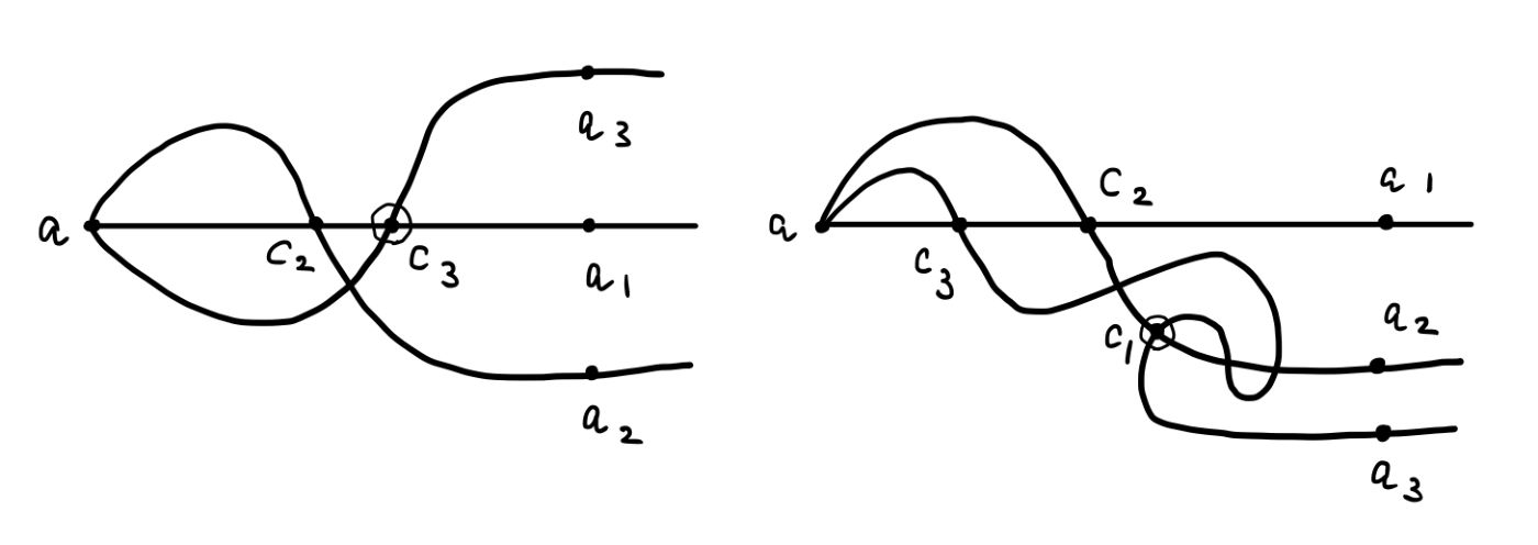
Case 2. $(\alpha_{3}(c_{3},a_{3})\backslash c_{3})\cap(\alpha_{2}(c_{2},a_{2})\backslash c_{2})\not=\emptyset$ . Then, let $c_{1}$ be the last point, along $\alpha_{3}$ , of the intersection $\alpha_{3}(c_{3},a_{3})\cap\alpha_{2}(c_{2},a_{2})$ . In this case, we take $c_{1}$ to be a vertex of the new theta curve and replace $\alpha_{i},i=1,2,3$ by

\alpha_{2}(c_{1},c_{2})\cup\alpha_{1}(c_{2},a_{1}),\alpha_{2}(c_{1},a_{2}),\alpha_{3}(c_{1},a_{3}).

(ii) Suppose $c_{3}\in\alpha_{1}(a,c_{2})$ . In this case, we replace $\alpha_{i}$ with $\alpha_{i}^{\prime}$ after we switch the roles of $\alpha_{2}$ and $\alpha_{3}$ , so that $c_{2}$ and $c_{3}$ are switched and we are in (i).

In all cases, any pair of $\alpha_{i}^{\prime}$ intersect only in the new vertex, and $(\alpha_{1}^{\prime}\cup\alpha_{2}^{\prime}\cup\alpha_{3}^{\prime})\subset(\alpha_{1}\cup\alpha_{2}\cup\alpha_{3})$ .

We replace $\beta_{i}$ similarly. Clearly we obtain in this way an $M$ -fat embedded theta curve. ∎

Definition ( $M$ -coarse cactus).

Let $X$ be a geodesic metric space. If there is an $M>0$ such that $X$ has no embedded, $M$ -fat theta curves then we say that $X$ is an $M$ -coarse cactus or simply a coarse cactus.

We give now a proof that a coarse cactus has asymptotic dimension at most one imitating the proof of Proposition2.1.

Theorem 3.2.

Let $C$ be an $M$ -coarse cactus. Then $\asdim C\leq 1$ . Moreover, it is uniform with $M$ fixed. Further, for any $m\geq M$ , we can take $D(m)=10^{5}m$ .

Note that, for $m<M$ , we could put, for example, $D(m)=10^{5}M$ , so that we can set $D(m)=10^{5}\max\{m,M\}$ for all $m$ .

Proof.

Let $m>0$ be given. It is enough to show that there is a covering of $C$ by uniformly bounded sets such that any ball of radius $m$ intersects at most 2 such sets. Without loss of generality we may assume $m\geq M$ . Fix $e\in C$ . Consider $f(x)=d(e,x)$ . We will pick $N=100m$ and consider the “annulus”

A_{k}=\{x|kN\leq f(x)<(k+1)N\}.

We define an equivalence relation on $A_{k}$ : $x\sim y$ if there are $x_{1}=x,x_{2},...,x_{n}=y$ such that $x_{i}\in A_{k}$ and $d(x_{i},x_{i+1})\leq 10m$ for all $i$ . Since every $x\in C$ lies in exactly one $A_{k}$ this equivalence relation is defined on all $C$ . Let’s denote by $B_{i}$ , $(i\in I)$ the equivalence classes of $\sim$ . By definition if $B_{i},B_{j}$ lie in some $A_{k}$ then a ball $B$ of radius $m$ intersects at most one of them. It follows that a ball of radius $m$ can intersect at most two equivalence classes. So it suffices to show that the $B_{i}$ ’s are uniformly bounded. We claim that $\diam(B_{i})\leq 1000N$ , which shows it suffices to take

D(m)=1000N=100000m.

We will argue by contradiction: let $x,y\in B_{i}\subseteq A_{k}$ such that $d(x,y)>1000N$ . We will show that there is an $N$ -fat theta curve in $C$ , which is a contradiction since $N>M$ , and Lemma 3.1 applies.

Since $\diam A_{k}\leq 2(k+1)N$ , we may assume $k\geq 499$ , so that $d(e,x)\geq 499N$ for $x\in A_{k}$ .

Let $\gamma_{1}:[0,\ell_{1}]\to C,\gamma_{3}:[0,\ell_{3}]\to C$ be geodesics (parametrized with respect to arc length) from $e$ to $x,y$ respectively.

By the definition of $\sim$ there is a path $\alpha:[0,\ell]\to C$ from $x$ to $y$ that lies in the $10m$ -neighborhood of $A_{k}$ . We further assume that $\alpha$ is simple. Let $a\in\alpha$ such that

d(a,x)=d(a,y).

Note $d(a,x)=d(a,y)>500N$ .

We consider a geodesic $\gamma_{2}:[0,\ell_{2}]\to C$ joining $e$ to $a$ . We claim that the theta curve

\Theta=\gamma_{1}\cup\gamma_{2}\cup\gamma_{3}\cup\alpha

with vertices $e,a$ is $N$ -fat. Explicitly the 3 arcs of $\Theta$ are $p_{1}=\gamma_{1}\cup\alpha(x,a)$ , $p_{2}=\gamma_{2}$ and $p_{3}=\gamma_{3}\cup\alpha(a,y)$ .

To see that $\Theta$ is $N$ -fat it is enough to define subarcs $p_{i}^{\prime}\subseteq p_{i}$ so that the conditions of the definition of $N$ -fat theta curves are satisfied.

We set $p_{i}^{\prime}=\gamma_{i}[\ell_{i}-20N,\ell_{i}-10N],i=1,2,3$ . We follow the notation of the definition of $M$ -fat theta curve, and we denote by $\alpha_{i},\beta_{i}$ ( $i=1,2,3)$ the arcs of the theta curve containing $a,e$ respectively. We verify the properties (1), (2), (3). Note that $(k-1)N\leq\ell_{i}\leq(k+2)N$ , and $499\leq k$ . Also,

\alpha\cap(p_{1}^{\prime}\cup p_{2}^{\prime}\cup p_{3}^{\prime}\cup\beta_{1}\cup\beta_{2}\cup\beta_{3})=\emptyset.

(1).If there are $s\in p_{i}^{\prime},t\in p_{j}^{\prime}$ such that $d(s,t)<N$ then it follows, by the triangle inequality, that $d(a,x)<20N+N+20N=41N$ or $d(a,y)<41N$ or $d(x,y)<41N$ which is a contradiction since $d(a,x)>500N$ , $d(a,y)>500N$ , and $d(x,y)>1000N$ . See Figure 3.

(2). In the case of $p_{1}^{\prime}$ , $p_{1}^{\prime}\cap\alpha_{1}=\emptyset,p_{1}^{\prime}\cap\beta_{1}=\emptyset$ is trivial by definition. If $p_{1}^{\prime}\cap\alpha_{2}\not=\emptyset$ , then $d(x,a)\leq 20N+10N=30N$ , impossible. If $p_{1}^{\prime}\cap\alpha_{3}\not=\emptyset$ then, $p_{1}^{\prime}\cap\alpha=\emptyset$ implies that $p_{1}^{\prime}\cap(\gamma_{3}\cap\alpha_{3})\not=\emptyset$ , so that $d(x,y)\leq 20N+10N=30N$ , impossible. If $p_{1}^{\prime}\cap\beta_{2}\not=\emptyset$ , then let $a^{\prime}\in\gamma_{2}$ be a point in the intersection. See Figure 3. Then $d(a,a^{\prime})\leq 22N$ . This is because

d(e,x)=d(e,a^{\prime})+d(a^{\prime},x)\leq d(e,a)-d(a,a^{\prime})+20N,

but since $|d(e,x)-d(e,a)|\leq 2N$ , we conclude $d(a,a^{\prime})\leq 22N$ . Therefore $d(a,x)\leq d(a,a^{\prime})+d(a^{\prime},x)\leq 22N+20N=42N$ , impossible. If $p_{1}^{\prime}\cap\beta_{3}\not=\emptyset$ , then $d(x,y)\leq 42N$ , impossible. We are done with $p_{1}^{\prime}$ .

In the case of $p_{2}^{\prime}$ . $p_{2}^{\prime}\cap\alpha_{2}=\emptyset,p_{2}^{\prime}\cap\beta_{2}=\emptyset$ is trivial. If $p_{2}^{\prime}\cap\alpha_{1}\not=\emptyset$ , then $d(a,x)\leq 20N+10N=30N$ , impossible (use $p_{2}^{\prime}\cap\alpha=\emptyset$ ). Same for $p_{2}^{\prime}\cap\alpha_{3}=\emptyset$ . If $p_{2}^{\prime}\cap\beta_{1}\not=\emptyset$ , then as we argued for $p_{1}^{\prime}\cap\beta_{2}=\emptyset$ , we would have $d(a,x)\leq 42N$ , impossible. The argument is same for $p_{2}^{\prime}\cap\beta_{3}=\emptyset$ . Therefore the condition holds for $p_{2}^{\prime}$ .

In the case of $p_{3}^{\prime}$ . The argument is exactly same as $p_{1}^{\prime}$ .

(3). If $t\in\alpha$ , then $d(e,t)\geq(k-1)N$ . If $t\in\alpha_{i}\cap\gamma_{i}$ for some $i$ , then

d(e,t)\geq\ell_{i}-10N\geq kN-11N.

So, if $t\in\alpha_{1}\cup\alpha_{2}\cup\alpha_{3}$ , then $d(e,t)\geq kN-11N$ . On the other hand, if $s\in\beta_{i}$ for some $i$ , then

d(e,s)\leq\ell_{i}-20N\leq kN-18N.

It follows that $d(t,s)\geq 7N\geq 700M$ . This completes the proof. ∎

We conclude this section with a lemma that is a consequence of the Jordan-Schoenflies curve theorem.

Lemma 3.3 (The theta-curve lemma).

Let $\Theta(p,q,r)$ be an embedded theta curve in $\mathbb{R}^{2}$ , and $e\in\mathbb{R}^{2}$ a point with $e\not\in\Theta$ . Then after swapping the labels $p,q,r$ if necessary, the simple loop $p\cup r$ divides $\mathbb{R}^{2}$ into two regions such that one contains $e$ and the other contains (the interior of) $q$ .

Proof.

By the Jordan-Schoenflies curve theorem (cf. [7]), after applying a self-homeomorphism of $\mathbb{R}^{2}$ , we may assume the simple loop $p\cup r$ is the unit circle in $\mathbb{R}^{2}$ , which divides the plane into two regions, $D_{1},D_{2}$ . If $e$ and $q$ are not in the same region, we are done. So, suppose both are in, say, $D_{1}$ . Then the arc $q$ divides $D_{1}$ into two regions, and call the one that contains $e$ , $D_{1}^{\prime}$ . After swapping $p,r$ if necessary, the boundary of $D_{1}^{\prime}$ is the simple loop $p\cup q$ . Now, apply the Jordan-Schoenflies curve theorem to the loop $p\cup q$ , then it divides the plane into two regions such that one is $D_{1}^{\prime}$ and the other one contains $r$ . Finally we swap $q,r$ and we are done. ∎

4. Asymptotic dimension of planar sets and graphs

Definition (Planar sets and graphs).

Let $(P,d_{P})$ be a geodesic metric space. We say it is a planar set if there is an injective continuous map,

\phi:P\to\mathbb{R}^{2}.

Let $P$ be a graph. We say $P$ is planar if there is an injective map

\phi:P\to\mathbb{R}^{2}

such that on each edge of $P$ , the map $\phi$ is continuous.

We view a connected graph as a geodesic space where each edge has length $1$ . We denote this metric by $d_{P}$ . We do not assume that the above map $\phi$ is continuous with respect to $d_{P}$ when $P$ is a graph.

4.1. Annuli are coarse-cacti

Let $(P,d_{P})$ be a geodesic metric space and pick a base point $e$ . For $r>m>0$ , set

A(r,r+m)=\{x\in P|r\leq d_{P}(e,x)<r+m\},

which we call an annulus, although it is not always a topological annulus.

We start with a key lemma.

Lemma 4.1.

Suppose $(P,d_{P})$ is a planar set or a planar graph. Then, for any $r,m>0$ , each connected component, $A$ , of $A(r,r+m)$ with the path metric $d_{A}$ has no embedded $m$ -fat theta curve.

Proof.

Case 1: Planar sets. We argue by contradiction. Suppose $A$ contains an embedded $m$ -fat theta-curve $\Theta(p,q,s)$ .

As we noted after the definition of a fat theta curve (recall $p^{\prime}\subset p$ ):

p\setminus N_{m}(q\cup s)\not=\emptyset,q\setminus N_{m}(s\cup p)\not=\emptyset,s\setminus N_{m}(p\cup q)\not=\emptyset.

Here, $N_{m}$ is for the open $m$ -neighborhood w.r.t. $d_{A}$ .

Using the map $\phi$ , we can identify $P$ with its image in $\mathbb{R}^{2}$ . Since $\Theta$ is (continuously) embedded by $\phi$ , we view it as a subset in $\mathbb{R}^{2}$ . Then by the theta-curve lemma (Lemma 3.3), after swapping $p,q,s$ if necessary, the simple loop $p\cup s$ divides $\mathbb{R}^{2}$ into two regions such that one contains $e$ and the other contains (the interior of) the arc $q$ .

Take a point

x\in q\setminus N_{m}(s\cup p).

Join $e$ and $x$ by a geodesic $\gamma$ in the space $P$ . Then by the Jordan curve theorem, $\gamma$ must intersect $p\cup s$ since $x\not\in D$ . See Figure 4.

Figure 4.

\gamma=[e,x]

must intersect

p\cup s

Let $y$ be a point on $\gamma$ that is on $p\cup s$ . Then

r\leq d_{P}(e,y)<r+m,\,\,r\leq d_{P}(e,x)<r+m,

so that $d_{P}(x,y)<m$ , and moreover the segment between $x,y$ on $\gamma$ is contained in $A$ , therefore $d_{A}(x,y)<m$ . It means $x$ is in the open $m$ -neighborhood of $p\cup s$ with respect to $d_{A}$ , which contradicts the way we chose $x$ .

Case 2: Planar graphs. The argument is almost same as the case 1, so we will be brief. We also keep the notations. Suppose $A$ contains an embedded $m$ -fat theta-curve $\Theta(p,q,s)$ . $\Theta$ contains only finitely many edges, so that $\phi|_{\Theta}$ is continuous. We proceed as before, and take a geodesic $\gamma$ in $P$ . Again, it contains only finitely many edges, so that $\phi|_{\gamma}$ is continuous and gives a path $\phi(\gamma)$ in $\mathbb{R}^{2}$ . So, $\gamma$ must intersect $p\cup s$ . The rest is same. ∎

We will show a few more lemmas. Although we keep the planar assumption, we only use the conclusion of Lemma 4.1, ie, no embedded, fat theta curves in annuli.

Lemma 4.2.

Suppose $(P,d_{P})$ is a planar set or a planar graph. Given $r,m>0$ , let $A$ be a connected component of $A(r,r+5m)$ , and $d_{A}$ its path metric. Then for any $L>0$ there is a constant $D(L)$ , which depends only on $L$ and $m$ , such that $(A,d_{A})$ has a cover by $D(L)$ -bounded sets whose $L$ -multiplicity is at most 2.

Moreover, we can take $D(L)=10^{5}\max\{L,5m\}.$

Proof.

Apply Lemma 4.1 to $A$ , then $(A,d_{A})$ has no embedded, $5m$ -fat theta curve. Namely, $(A,d_{A})$ is a $5m$ -coarse cactus. Then, Theorem 3.2 implies that a desired constant $D(L)$ exists, which depends only on $L,m$ . The moreover part is also from the theorem. ∎

4.2. Asymptotic dimension of a plane

Lemma 4.2 implies a similar result with respect to the metric $d_{P}$ for $L=m$ if we reduce the width of the annulus:

Lemma 4.3.

Suppose $(P,d_{P})$ is a planar set or a planar graph. Given $r,m>0$ , let $A_{1}(r,r+3m)$ be a connected component of $A(r,r+3m)$ . Then there is a cover of $(A_{1}(r,r+3m),d_{P})$ , by $(10^{6}m)$ -bounded sets whose $m$ -multiplicity is at most $2$ .

Proof.

Let $A_{1}(r-m,r+4m)$ be the connected component of $A(r-m,r+4m)$ that contains $A_{1}(r,r+3m)$ . Apply the lemma 4.2 to $A_{1}(r-m,r+4m)$ with the path metric, setting $L=m$ , and obtain a cover whose $m$ -multiplicity is at most $2$ by $(10^{6}m)$ -bounded sets. Restrict the cover to $A_{1}(r,r+3m)$ . We argue this is a desired cover. First, this cover is $10^{6}m$ -bounded w.r.t. $d_{P}$ . That is clear since $d_{P}$ is not larger than the path metric on $A_{1}(r-m,r+4m)$ .

Also, its $m$ -multiplicity is 2 w.r.t. $d_{P}$ . To see it, let $x\in A_{1}(r,r+3m)$ be a point. Suppose $K$ is a set in the cover with $d_{P}(x,K)\leq m$ . Then a path that realizes the distance $d_{P}(x,K)$ is contained in $A_{1}(r-m,r+4m)$ , so that the distance between $x$ and $K$ is at most $m$ w.r.t. the path metric on $A_{1}(r-m,r+4m)$ . But there are at most 2 such $K$ for a given $x$ , and we are done. ∎

Lemma 4.3 implies a lemma for the entire annulus, if we reduce the width further, which is in general not connected.

Lemma 4.4.

Suppose $(P,d_{P})$ is a planar set or a planar graph. Then, for any $r,m>0$ , there is a cover of $(A(r,r+m),d_{P})$ by $(10^{6}m)$ -bounded sets whose $m$ -multiplicity is at most 2.

Figure 5. The shaded area in

A_{k}(r,r+3m)

A_{k}(r+m,r+2m)

for

k=i,j

[x,x^{\prime}]\subset A_{i}(r,r+3m),[y,y^{\prime}]\subset A_{j}(r,r+3m)

Proof.

We will construct a desired covering for $(A(r+m,r+2m),d_{P})$ , then rename $r+m$ by $r$ . (Strictly speaking, this renaming works only for $r>m$ . But if $r\leq m$ , then the diameter of $A(r,r+m)$ is $\leq 4m$ , so that the conclusion holds.)

The metric in the argument is $d_{P}$ unless otherwise said.

Let $A_{1}(r,r+3m)$ be a connected component of $A(r,r+3m)$ . By lemma 4.3, we have a covering of $(A_{1}(r,r+3m),d_{P})$ by $(10^{6}m)$ -bounded sets whose $m$ -multiplicity is 2. Then restrict the covering to the set

A_{1}(r+m,r+2m)=A_{1}(r,r+3m)\cap A(r+m,r+2m).

Apply the same argument to all other components, $A_{i}(r,r+3m)$ , of $A(r,r+3m)$ , and obtain a covering for

A_{i}(r+m,r+2m)=A_{i}(r,r+3m)\cap A(r+m,r+2m).

So far, we obtained a desired covering for each $A_{i}(r+m,r+2m)$ .

Consider the following decomposition,

A(r+m,r+2m)=\sqcup_{i}A_{i}(r+m,r+2m).

We will obtain a desired covering on the left hand side by gathering the covering we have for each set on the right hand side. We are left to verify that the sets $A_{i}(r+m,r+2m)$ ’s are $2m$ -separated from each other w.r.t. $d_{P}$ .

Indeed, let $A_{i}(r+m,r+2m),A_{j}(r+m,r+2m)$ be distinct sets. Then

A_{i}(r+m,r+2m)\subset A_{i}(r,r+3m),A_{j}(r+m,r+2m)\subset A_{j}(r,r+3m),

A_{i}(r,r+3m)\cap A_{j}(r,r+3m)=\emptyset.

Now, take a point $x\in A_{i}(r+m,r+2m)$ and a point $y\in A_{j}(r+m,r+2m)$ . Join $x,y$ by a geodesic, $\gamma$ , in $P$ . See Figure 5. Let $x^{\prime}\in\gamma$ be the first point where $\gamma$ exits $A_{i}(r,r+3m)$ . Then we have $d_{P}(x,x^{\prime})\geq m.$ Let $y^{\prime}\in\gamma$ be the last point where $\gamma$ enters $A_{j}(r,r+3m)$ . Then $d_{P}(y^{\prime},y)\geq m$ . Since $A_{i}(r,r+3m)$ and $A_{j}(r,r+3m)$ are disjoint,

d_{P}(x,y)>d_{P}(x,x^{\prime})+d_{P}(y^{\prime},y)=2m.

∎

4.3. Proof of Theorems 1.1, 1.2 and Corollary 1.3

We prove Theorems 1.1 and 1.2 at one time.

Proof.

By assumption, $(P,d_{P})$ is either a planar set (Theorem 1.1) or a planar graph (Theorem 1.2). Given $m>0$ , define annuli

A_{n}=A(nm,(n+1)m),n\geq 0.

Set $D(m)=10^{6}m$ . By Lemma 4.4 each $(A_{n},d_{P})$ has a covering by $D(m)$ -bounded sets whose $m$ -multiplicity is at most 2.

Gathering all of the coverings for the annuli, we have a covering of $(P,d_{P})$ by $D(m)$ -bounded sets whose $\frac{m}{3}$ -multiplicity is at most 4 since any ball of radius $\frac{m}{3}$ intersect at most two annuli as $A_{n}$ and $A_{n+2}$ are at least $m$ -apart for all $n$ with respect to $d_{P}$ . We are done by renaming $\frac{m}{3}$ by $m$ , and changing $D(m)$ to $D(m)=3(10^{6}m)$ accordingly. ∎

There is nothing more to argue for Corollary 1.3 since it is only a special case of Theorem 1.2 for finite graphs.

5. Questions and remarks

An obvious open question is the following:

Question 5.1.

Is the asymptotic dimension of a plane at most two for any geodesic metric?

Note added in proof. Jørgensen-Lang [16] have answered the question affirmatively by now. An argument goes like this (slightly different from [16]). For a map $f:X\to Y$ between metric spaces, Brodskiy-Dydak-Levin-Mitra [6] introduced the notion of the asymptotic dimension of $f$ , $\asdim f$ , and proved a Hurewicz type theorem, [6, Theorem 4.11]: $\asdim X\leq\asdim f+\asdim Y$ . Now apply this to the distance function from a base point, $f:P\to\mathbb{R}$ . Using Lemma 4.4 one argues $\asdim f\leq 1$ , and since $\asdim\mathbb{R}=1$ , it follows $\asdim P\leq 2$ . This is only for the asymptotic dimension, and they [16] showed the Assouad-Nagata dimension of $P$ is at most 2 by exhibiting a linear bound for $D(m)$ . Also, concerning Question 5.1 another proof of a slightly more general result is given by Bonamy-Bousquet-Esperet-Groenland-Pirot-Scott [3].

It is reasonable to ask whether the asymptotic bound for minor excluded graphs is uniform:

Question 5.2.

Given $m\geq 3$ , is there an $M>0$ such that if $\Gamma$ be a connected graph excluding the complete graph $K_{m}$ as a minor then $\Gamma$ has asymptotic dimension at most $M$ ? In fact one may ask whether it is possible to take $M=2$ .

Note added in proof. Bonamy et al [3] have answered this by now in the bounded degree case and Liu [19] in general.

In contrast to Theorem 1.1,

Proposition 5.3.

$\mathbb{R}^{3}$ has a Riemannian metric whose asymptotic dimension is infinite.

Probably this result is known to experts but we give a proof as we did not find it in the literature. Note that any finite graph can be embedded in $\mathbb{R}^{3}$ and one sees easily that by changing the metric one can make these embeddings say $(2,2)$ quasi-isometric. Indeed one may take a small neighborhood of the graph and define a metric so that the distance from an edge to the surface of this neighborhood is sufficiently large. Fix $n>3$ and take a unit cubical grid in $\mathbb{R}^{n}$ , then consider a sequence of finite subgraphs $\Gamma_{i}$ in the grid of size $i>0$ . We join $\Gamma_{i}$ with $\Gamma_{i+1}$ by an edge (for all $i$ ) and we obtain an infinite graph, $\Lambda^{n}$ , whose asymptotic dimension is equal to $n$ . This graph also embeds in $\mathbb{R}^{3}$ and one can arrange a Riemannian metric on $\mathbb{R}^{3}$ such that the embedding is $(2,2)$ quasi-isometric. For this metric the asymptotic dimension of $\mathbb{R}^{3}$ is at least $n$ . Finally we can embed the disjoint union of $\Lambda^{n},n>3$ in $\mathbb{R}^{3}$ and arrange a Riemannian metric on $\mathbb{R}^{3}$ such that the embedding is $(2,2)$ quasi-isometric. Now the asymptotic dimension of $\mathbb{R}^{3}$ is infinite for this metric.

References

[1] K. Appel, W. Haken. Every planar map is four colorable. Bulletin of the American mathematical Society. 1976;82(5):711-712.
[2] C. Bavard, P. Pansu. Sur le volume minimal de ${R}^{2}$ . Annales scientifiques de l’Ecole Normale Supérieure 1986. Vol. 19, No. 4, 479-490.
[3] M. Bonamy, N. Bousquet, L. Esperet, C. Groenland, F. Pirot and A. Scott. Surfaces have (asymptotic) dimension 2. preprint 2020. arXiv:2007.03582.
[4] I. Benjamini, J. Cao. A new isoperimetric comparison theorem for surfaces of variable curvature. Duke Mathematical Journal. 1996;85(2):359-396.
[5] B. H.Bowditch, ”The minimal volume of the plane.” Journal of the Australian Mathematical Society 55, no. 1 (1993): 23-40.
[6] N. Brodskiy, J. Dydak, M. Levin, A. Mitra. A Hurewicz theorem for the Assouad-Nagata dimension. J. Lond. Math. Soc. (2) 77 (2008), no. 3, 741-–756.
[7] Stewart S. Cairns, An elementary proof of the Jordan-Schoenflies theorem. Proc. Amer. Math. Soc. 2 (1951), 860-–867.
[8] G. A. Dirac and S. Schuster, A theorem of Kuratowski, Indagationes Math. 16 (1954) 343–-348.
[9] J.R.Gilbert, J.P. Hutchinson, R.E. Tarjan A separator theorem for graphs of bounded genus J. Algorithms 5 (1984) 391-407.
[10] M.Gromov, Asymptotic invariants of infinite groups, in Geometric Group Theory, v. 2, 1-295, London Math. Soc. Lecture Note Ser., vol. 182, Cambridge Univ. Press, Cambridge, 1993.
[11] R. Grimaldi, P. Pansu.Remplissage et surfaces de revolution. Journal de mathématiques pures et appliquées. 2003;82(8):1005-1046.
[12] Frank Harary, George E.Uhlenbeck, On the number of Husimi trees. I. Proc. Nat. Acad. Sci. U.S.A. 39 (1953), 315-–322.
[13] J.Hass Isoperimetric regions in nonpositively curved manifolds. preprint 2016. arXiv:1604.02768.
[14] J.Hersch, Quatre proprietes isoperimetriques de membranes spheriques homogenes, C.R. Acad. Sci. Paris 270 (1970) 1645-1648
[15] Hugh Howards, Michael Hutchings, Frank Morgan (1999)The Isoperimetric Problem on Surfaces, The American Mathematical Monthly, 106:5, 430-439
[16] Martina Jørgensen, Urs Lang. Geodesic spaces of low Nagata dimension. preprint, 2020, arXiv:2004.10576
[17] P.Klein, S.A.Plotkin, and S. Rao, Excluded minors, network decomposition, and multicommodity flow. In Proceedings of the twenty-fifth annual ACM symposium on Theory of computing ( 682-690).1993, June.
[18] RJ. Lipton , RE. Tarjan .A separator theorem for planar graphs. SIAM Journal on Applied Mathematics. 1979;36(2):177-89.
[19] C.H.Liu, Asymptotic dimension of minor-closed families and beyond. preprint 2020.arXiv:2007.08771.
[20] F. Morgan, M.Hutchings, H.Howards The isoperimetric problem on surfaces of revolution of decreasing Gauss curvature. Transactions of the American Mathematical Society. 2000;352(11):4889-909.
[21] T. Nishizeki, N. Chiba Planar graphs: Theory and algorithms. North-Holland Mathematics Studies, 140. 1988
[22] Mikhail I. Ostrovskii, David Rosenthal, Metric dimensions of minor excluded graphs and minor exclusion in groups. Internat. J. Algebra Comput. 25 (2015), no. 4, 541–-554.
[23] M.Ritoré The isoperimetric problem in complete surfaces of nonnegative curvature. The Journal of Geometric Analysis. 2001, 11(3):509–517.
[24] W.T.Tutte, A theorem on planar graphs. Transactions of the American Mathematical Society, 82(1), 99-116.1956.

Asymptotic dimension of planes and planar graphsThanks: The first author is supported in part by Grant-in-Aid for Scientific Research (No. 15H05739, 20H00114). He would like to thank Mathematical Institute of University of Oxford for their hospitality.

Abstract.

1. Introduction

1.1. Statements

Theorem 1.1.

Theorem 1.2.

Corollary 1.3.

Theorem 1.4 (Ostrovskii-Rosenthal).

1.2. Idea of proofs

Acknowledgements

2. Asymptotic dimension of cacti

2.1. Cactus

Definition (Cactus).

Proposition 2.1.

Proof.

Corollary 2.2.

3. Coarse cacti

Definition (MM-fat theta curve).

Lemma 3.1.

Proof.

Definition (MM-coarse cactus).

Theorem 3.2.

Proof.

Lemma 3.3 (The theta-curve lemma).

Proof.

4. Asymptotic dimension of planar sets and graphs

Definition (Planar sets and graphs).

4.1. Annuli are coarse-cacti

Lemma 4.1.

Proof.

Lemma 4.2.

Proof.

4.2. Asymptotic dimension of a plane

Lemma 4.3.

Proof.

Lemma 4.4.

Proof.

4.3. Proof of Theorems 1.1, 1.2 and Corollary 1.3

Proof.

5. Questions and remarks

Question 5.1.

Question 5.2.

Proposition 5.3.

References

Definition ( $M$ -fat theta curve).

Definition ( $M$ -coarse cactus).