跳到论文正文
W Papers独立论文阅读器 arXiv:2002.01503 论文正文 计算阅读时间 · 0%
引用这篇论文根据当前论文元数据生成,正式投稿前建议核对。


License: arXiv.org perpetual non-exclusive license
arXiv:2002.01503v1 [math.DS] 04 Feb 2020

Solution estimates for linear differential equations with delayJournal: Applied Mathematics and Computation

Leonid Berezansky Address: Dept. of Math., Ben-Gurion University of the Negev, Beer-Sheva 84105, Israel    Elena Braverman Address: Dept. of Math. and Stats., University of Calgary,2500 University Drive N.W., Calgary, AB, Canada T2N 1N4; e-mail maelena@ucalgary.ca, phone 1-(403)-220-3956, fax 1-(403)–282-5150 (corresponding author)
Abstract

In this paper, we give explicit exponential estimates |x⁡(t)|≤M​e−γ⁡(t−t0)\displaystyle|x(t)|\leq Me^{-\gamma(t-t_{0})}, where t≥t0t\geq t_{0}, M>0M>0, for solutions of a linear scalar delay differential equation

x˙​(t)+∑k=1mbk​(t)​x​(hk​(t))=f⁡(t),t≥t0,x⁡(t)=ϕ⁡(t),t≤t0.\dot{x}(t)+\sum_{k=1}^{m}b_{k}(t)x(h_{k}(t))=f(t),~~t\geq t_{0},~x(t)=\phi(t),~t\leq t_{0}.

We consider two different cases: when γ>0\gamma>0 (corresponding to exponential stability) and the case of γ<0\gamma<0 when the solution is, generally, growing.

In the first case, together with the exponential estimate, we also obtain an exponential stability test, in the second case we get estimation for solution growth. Here both the coefficients and the delays are measurable, not necessarily continuous.

Keywords: 
linear delay differential equations, explicit solution estimates, variable delays and coefficients, exponential stability AMS subject classification: 34K20, 34K25, 34K06

1 Introduction

Exponential or asymptotic stability of solutions is one of the most important properties of a functional differential equation (FDE). There are many publications on stability of a FDE. We cite here the papers [6, 7, 8, 9, 16, 17, 18, 22, 26, 28] and the monographs [4, 13, 14, 15, 21] fully or partially devoted to asymptotic stability of this class of equations. Asymptotic stability describes long time behavior of solutions. But in applications of FDEs, usually it is necessary to know estimates of solutions on finite intervals. The following well-known topics are close to one considered in the paper: Lyapunov exponents, asymptotic integration, and growth rates [2, 3, 5, 10, 11, 12, 19, 20, 23, 24, 25, 27].

In this paper, we propose exponential estimates for solutions of a scalar delay differential equation (DDE) with variable coefficients and delays

x˙(t)+∑k=1mbk(t)x(hk(t))=0,t≥t0,hk(t)≤t,k=1,…,m.\dot{x}(t)+\sum_{k=1}^{m}b_{k}(t)x(h_{k}(t))=0,~~t\geq t_{0},~h_{k}(t)\leq t,~k=1,\dots,m. (1.1)

Estimates for non-homogeneous equations are also considered. We investigate two different cases, one when the equation is exponentially stable and the second when it is not, or when asymptotic behaviour of solutions is unknown.

For the equation with one delay

x˙​(t)+a⁡(t)​x​(h⁡(t))=0,\dot{x}(t)+a(t)x(h(t))=0,

for example, the first case occurs when a⁡(t)≥a0>0a(t)\geq a_{0}>0 and the equation is exponentially stable, the second case is for a⁡(t)≥0a(t)\geq 0 but the equation is not exponentially stable, or for a⁡(t)a(t) being non-positive or oscillatory.

All our conditions can be applied to a wide class of scalar linear differential equations with variable coefficients and delays, without the assumption that these parameters are continuous functions, leading to solution estimates. For equations with variable coefficients and delays, such solution estimates are obtained for the first time, and for ordinary differential equations are sharp.

The paper is organized as follows. After some definitions and auxiliary results in Section 2, Section 3 contains an estimate for the fundamental function of an equation with a non-delay term. Section 4 is the main part of the paper. Here we consider solution estimates in the two above mentioned cases. Section 5 presents illustrating examples. Section 6 contains a discussion and suggests some projects for future research.

2 Preliminaries

We consider equation (1.1) under the following conditions:

(a1) bk:[0,∞)→ℝb_{k}:[0,\infty)\to{\mathbb{R}} are Lebesgue measurable essentially bounded functions;

(a2) the functions hkh_{k} are Lebesgue measurable on [0,∞)[0,\infty), and for some finite constants δk≤τk\delta_{k}\leq\tau_{k}, 0≤δk≤t−hk​(t)≤τk0\leq\delta_{k}\leq t-h_{k}(t)\leq\tau_{k}, k=1,…,mk=1,\dots,m, t≥t0≥0t\geq t_{0}\geq 0, τ=maxk⁡τk\tau=\max_{k}\tau_{k}.

Together with equation (1.1), we consider for any t0≥0t_{0}\geq 0 an initial value problem for the non-homogeneous equation

x˙​(t)+∑k=1mbk​(t)​x​(hk​(t))=f⁡(t),t≥t0;x⁡(t)=ϕ⁡(t),t≤t0,\dot{x}(t)+\sum_{k=1}^{m}b_{k}(t)x(h_{k}(t))=f(t),~t\geq t_{0};~~x(t)=\phi(t),~t\leq t_{0}, (2.1)

where
(a3) f:[t0,∞)→ℝf:[t_{0},\infty)\to{\mathbb{R}} is a Lebesgue measurable locally essentially bounded function, the initial function ϕ:[t0−τ,t0]→ℝ\phi:[t_{0}-\tau,t_{0}]\rightarrow{\mathbb{R}} is bounded and Borel measurable.

By the solution of problem (2.1) we mean a locally absolutely continuous function x:[t0,∞)→ℝx:[t_{0},\infty)\to{\mathbb{R}} satisfying almost everywhere the equation, whenever t≥t0t\geq t_{0}, and the initial conditions if t≤t0t\leq t_{0}.

For any fixed ss, the solution X⁡(t,s)X(t,s) of the problem with the zero initial function and the initial value being equal to one

∂X⁡(t,s)∂t+∑k=1mbk​(t)​X​(hk​(t),s)=0,t≥s;X⁡(t,s)=0,t<s,X⁡(s,s)=1\frac{\partial X(t,s)}{\partial t}+\sum_{k=1}^{m}b_{k}(t)X(h_{k}(t),s)=0,~t\geq s;~~X(t,s)=0,~t<s,~~X(s,s)=1

is called the fundamental function.

According to [4, Theorem 4.3.1], the solution of (2.1) exists and is unique. Also, the solution has the representation

x⁡(t)=X⁡(t,t0)​x​(t0)−∑k=1m∫t0t0+τkX⁡(t,s)​bk​(s)​ϕ​(hk​(s))​𝑑s+∫t0tX⁡(t,s)​f​(s)​𝑑s.x(t)=X(t,t_{0})x(t_{0})-\sum_{k=1}^{m}\int_{t_{0}}^{t_{0}+\tau_{k}}X(t,s)b_{k}(s)\phi(h_{k}(s))ds+\int_{t_{0}}^{t}X(t,s)f(s)ds. (2.2)

In (2.2), we assume ϕ⁡(t)=0\phi(t)=0, t>t0t>t_{0}.

We call equation (1.1) uniformly exponentially stable if, for some positive numbers MM and γ\gamma, not depending on t0t_{0} and ϕ\phi, a solution of homogeneous (2.1), where f≡0f\equiv 0, satisfies

|x⁡(t)|≤M​e−γ⁡(t−t0)​supt∈[t0−τ,t0]|ϕ⁡(t)|,t≥t0.|x(t)|\leq Me^{-\gamma(t-t_{0})}\sup_{t\in[t_{0}-\tau,t_{0}]}|\phi(t)|,~~t\geq t_{0}. (2.3)

We will say that the fundamental function X⁡(t,s)X(t,s) of (1.1) has an exponential estimate if there exist M0>0M_{0}>0 and γ0>0\gamma_{0}>0 such that

|X⁡(t,s)|≤M0​e−γ0​(t−s), for any ​t≥s≥0.|X(t,s)|\leq M_{0}e^{-\gamma_{0}(t-s)},\mbox{~~for any~~~}t\geq s\geq 0. (2.4)

We will further apply the Bohl-Perron theorem stated below.

Lemma 1.

[4, Theorem 4.7.1] Assume that (a1)-(a2) hold. If the solution of the problem

x˙​(t)+∑k=1mbk​(t)​x​(hk​(t))=f⁡(t),x⁡(t)=0,t≤t0\dot{x}(t)+\sum_{k=1}^{m}b_{k}(t)x(h_{k}(t))=f(t),~x(t)=0,~t\leq t_{0} (2.5)

is bounded on [t0,∞)[t_{0},\infty) for any essentially bounded function f:[t0,∞)→ℝf:[t_{0},\infty)\to{\mathbb{R}}, equation (1.1) is uniformly exponentially stable.

The main objective of the present paper is to obtain explicit estimates (2.3)-(2.4) and their generalizations for homogeneous equation (1.1). We consider the case when the equation is exponentially stable and when it is unstable, or asymptotic behaviour is unknown. In the former case γ>0\gamma>0, while in the latter case γ<0\gamma<0. We also get estimates for non-homogeneous equations (2.1).

3 Estimates for an Auxiliary Equation

In this section, for the fundamental function Y⁡(t,s)Y(t,s) of the equation involving both delay terms and a non-delay term

y˙​(t)=c⁡(t)​y​(t)−∑k=1mdk​(t)​y​(hk​(t)),t≥t0\dot{y}(t)=c(t)y(t)-\sum_{k=1}^{m}d_{k}(t)y(h_{k}(t)),~t\geq t_{0} (3.1)

we deduce a uniform estimate

|Y⁡(t,s)|≤K​ for ​t≥s≥t0.|Y(t,s)|\leq K\mbox{~~for~~}t\geq s\geq t_{0}. (3.2)

We assume that for c,dkc,d_{k}, assumption (a1) holds, while the delay functions hkh_{k} satisfy (a2).

Denote ‖f‖J=ess​supt∈J⁡|f⁡(t)|\|f\|_{J}=\esssup_{t\in J}|f(t)|, where J=[t0,t1]J=[t_{0},t_{1}] or J=[t0,∞)J=[t_{0},\infty), d⁡(t):=∑k=1mdk​(t)\displaystyle d(t):=\sum_{k=1}^{m}d_{k}(t).

Lemma 2.

If there is an α0>0\alpha_{0}>0 such that

d⁡(t)−c⁡(t)≥α0,K0:=(‖c‖[t0,∞)+∑k=1m‖dk‖[t0,∞))​∑k=1mτk​‖dkd−c‖[t0,∞)<1d(t)-c(t)\geq\alpha_{0},~~K_{0}:=\left(\|c\|_{[t_{0},\infty)}+\sum_{k=1}^{m}\|d_{k}\|_{[t_{0},\infty)}\right)\sum_{k=1}^{m}\tau_{k}\left\|\frac{d_{k}}{d-c}\right\|_{[t_{0},\infty)}<1 (3.3)

then (3.1) is uniformly exponentially stable. Moreover, the fundamental function Y⁡(t,s)Y(t,s) of (3.1) satisfies (3.2) with K=(1−K0)−1.K=(1-K_{0})^{-1}.

Proof.

For brevity of notations, we set y⁡(t)=Y⁡(t,t0)y(t)=Y(t,t_{0}). Then, yy satisfies (3.1), where the initial value is y⁡(t0)=1y(t_{0})=1, with the zero initial function. Let J=[t0,t1]J=[t_{0},t_{1}], where t1>t0t_{1}>t_{0} is arbitrary. Equality (3.1) implies the estimate

‖y˙‖J≤(‖c‖[t0,∞)+∑k=1m‖dk‖[t0,∞))​‖y‖J.\|\dot{y}\|_{J}\leq\left(\|c\|_{[t_{0},\infty)}+\sum_{k=1}^{m}\|d_{k}\|_{[t_{0},\infty)}\right)\|y\|_{J}. (3.4)

Equation (3.1) can be written as

y˙​(t)=−[d⁡(t)−c⁡(t)]​y​(t)+∑k=1mdk​(t)​∫hk​(t)ty˙​(ξ)​𝑑ξ.\dot{y}(t)=-[d(t)-c(t)]y(t)+\sum_{k=1}^{m}d_{k}(t)\int_{h_{k}(t)}^{t}\dot{y}(\xi)d\xi.

Integrating, we get for yy

y(t)=e−∫t0t[d(ξ)−c(ξ)]dξ+∫t0te−∫st[d(ξ)−c(ξ)]dξ[d(s)−c(s)][∑k=1mdk​(s)d⁡(s)−c⁡(s)∫hk​(s)sy˙(ξ)dξ]ds.y(t)=e^{-\int_{t_{0}}^{t}[d(\xi)-c(\xi)]d\xi}+\int_{t_{0}}^{t}e^{-\int_{s}^{t}[d(\xi)-c(\xi)]d\xi}[d(s)-c(s)]\left[\sum_{k=1}^{m}\frac{d_{k}(s)}{d(s)-c(s)}\int_{h_{k}(s)}^{s}\dot{y}(\xi)d\xi\right]ds.

Then, by the above equality, (3.4) and the definition of K0K_{0} in (3.3),

‖y‖J≤1+∑k=1mτk​‖dkd−c‖[t0,∞)​‖y˙‖J≤1+K0​‖y‖J.\|y\|_{J}\leq 1+\sum_{k=1}^{m}\tau_{k}\left\|\frac{d_{k}}{d-c}\right\|_{[t_{0},\infty)}\|\dot{y}\|_{J}\leq 1+K_{0}\|y\|_{J}.

Then ‖Y⁡(t,t0)‖J≤(1−K0)−1\|Y(t,t_{0})\|_{J}\leq(1-K_{0})^{-1}, and the expression in the right-hand side does not depend on t1t_{1}.

Hence ‖Y⁡(t,t0)‖[t0,∞)≤(1−K0)−1\displaystyle\|Y(t,t_{0})\|_{[t_{0},\infty)}\leq(1-K_{0})^{-1}. Again, the number in the right-hand side does not depend on t0t_{0}. Thus estimate (3.2) holds.

To prove exponential stability, we apply the Bohl-Perron theorem. Let f:[t0,∞)→ℝf:[t_{0},\infty)\to{\mathbb{R}} be globally essentially bounded, and yy be a solution of

y˙​(t)=c⁡(t)​y​(t)−∑k=1mdk​(t)​y​(hk​(t))+f⁡(t),t≥t0,y⁡(t)=0,t≤t0.\dot{y}(t)=c(t)y(t)-\sum_{k=1}^{m}d_{k}(t)y(h_{k}(t))+f(t),~t\geq t_{0},~y(t)=0,t\leq t_{0}. (3.5)

Equality (3.5) implies

‖y˙‖J≤(‖c‖[t0,∞)+∑k=1m‖dk‖[t0,∞))​‖y‖J+‖f‖[t0,∞).\|\dot{y}\|_{J}\leq\left(\|c\|_{[t_{0},\infty)}+\sum_{k=1}^{m}\|d_{k}\|_{[t_{0},\infty)}\right)\|y\|_{J}+\|f\|_{[t_{0},\infty)}. (3.6)

Similarly to the above argument, equation (3.5) can be rewritten and integrated:

y˙​(t)=\displaystyle\dot{y}(t)= −[d⁡(t)−c⁡(t)]​y​(t)+∑k=1mdk​(t)​∫hk​(t)ty˙​(ξ)​𝑑ξ+f⁡(t),\displaystyle-[d(t)-c(t)]y(t)+\sum_{k=1}^{m}d_{k}(t)\int_{h_{k}(t)}^{t}\dot{y}(\xi)d\xi+f(t),
y⁡(t)=\displaystyle y(t)= ∫t0te−∫st[d(ξ)−c(ξ)]dξ[d(s)−c(s)][∑k=1mdk​(s)d⁡(s)−c⁡(s)∫hk​(s)sy˙(ξ)dξ]ds\displaystyle\int_{t_{0}}^{t}e^{-\int_{s}^{t}[d(\xi)-c(\xi)]d\xi}[d(s)-c(s)]\left[\sum_{k=1}^{m}\frac{d_{k}(s)}{d(s)-c(s)}\int_{h_{k}(s)}^{s}\dot{y}(\xi)d\xi\right]\,ds
+∫t0te−∫st[d(ξ)−c(ξ)]dξ[d(s)−c(s)]f⁡(s)d⁡(s)−c⁡(s)ds.\displaystyle+\int_{t_{0}}^{t}e^{-\int_{s}^{t}[d(\xi)-c(\xi)]d\xi}[d(s)-c(s)]\frac{f(s)}{d(s)-c(s)}\,ds.

Since d⁡(s)−c⁡(s)≥α0>0d(s)-c(s)\geq\alpha_{0}>0 and ‖f‖[t0,∞)<∞\|f\|_{[t_{0},\infty)}<\infty, we have ‖fd−c‖[t0,∞)<∞\|\frac{f}{d-c}\|_{[t_{0},\infty)}<\infty. Then, by (3.6),

‖y‖J≤∑k=1mτk​‖dkd−c‖[t0,∞)​‖y˙‖J+‖fd−c‖[t0,∞)≤K0​‖y‖J+M0,\|y\|_{J}\leq\sum_{k=1}^{m}\tau_{k}\left\|\frac{d_{k}}{d-c}\right\|_{[t_{0},\infty)}\|\dot{y}\|_{J}+\left\|\frac{f}{d-c}\right\|_{[t_{0},\infty)}\leq K_{0}\|y\|_{J}+M_{0},

where

M0=∑k=1mτk​‖dkd−c‖[t0,∞)​‖f‖[t0,∞)+‖fd−c‖[t0,∞).M_{0}=\sum_{k=1}^{m}\tau_{k}\left\|\frac{d_{k}}{d-c}\right\|_{[t_{0},\infty)}\|f\|_{[t_{0},\infty)}+\left\|\frac{f}{d-c}\right\|_{[t_{0},\infty)}.

Hence for the constant M=(1−K0)−1​M0>0M=(1-K_{0})^{-1}M_{0}>0, we have ‖y‖J≤M\|y\|_{J}\leq M, where MM does not depend on the interval JJ. Therefore ‖x‖[t0,∞)<∞\|x\|_{[t_{0},\infty)}<\infty. Appliing Lemma 1, we conclude that (3.1) is uniformly exponentially stable. ∎

Remark 1.

In Lemma 2, instead of K0K_{0}, we can take any number K1∈(K0,1)K_{1}\in(K_{0},1).

Remark 2.

Equation (3.1) is uniformly exponentially stable under the assumptions of the lemma. In contrast to a known result on exponential stability of an equation y˙+c⁡(t)​y​(t)+d⁡(t)​y​(h⁡(t))=0\dot{y}+c(t)y(t)+d(t)y(h(t))=0 with a dominating non-delay term c⁡(t)>|d⁡(t)|≥0c(t)>|d(t)|\geq 0, we consider the case c⁡(t)≤0c(t)\leq 0, d⁡(t)>c⁡(t)d(t)>c(t). In this sense, the delay term is dominating over the non-delay term.

4 Main Results

4.1 Exponentially stable equations

We start with an exponential estimate for an exponentially stable equation.

Theorem 1.

Assume that there are constants λ>0\lambda>0 and α>0\alpha>0 such that the following inequalities hold:

a⁡(t):=∑k=1meλ​(t−hk​(t))​bk​(t)−λ≥α,t≥t0,a(t):=\sum_{k=1}^{m}e^{\lambda(t-h_{k}(t))}b_{k}(t)-\lambda\geq\alpha,\quad t\geq t_{0}, (4.1)
M1:=(λ+∑k=1meλ​τk​‖bk‖[t0,∞))​∑k=1mτk​‖aka‖[t0,∞)<1,M_{1}:=\left(\lambda+\sum_{k=1}^{m}e^{\lambda\tau_{k}}\|b_{k}\|_{[t_{0},\infty)}\right)\sum_{k=1}^{m}\tau_{k}\left\|\frac{a_{k}}{a}\right\|_{[t_{0},\infty)}<1, (4.2)

where ak​(t)=eλ​(t−hk​(t))​bk​(t)a_{k}(t)=e^{\lambda(t-h_{k}(t))}b_{k}(t).

Then for the solution of problem (2.1), the following estimate is valid

|x⁡(t)|≤M0​e−λ⁡(t−t0)​[|x⁡(t0)|+∑k=1meλ​τk−1λ​‖bk‖[t0,∞)​‖ϕ‖[t0−τ,t0]]+M0λ​‖f‖[t0,t],|x(t)|\leq M_{0}e^{-\lambda(t-t_{0})}\left[|x(t_{0})|+\sum_{k=1}^{m}\frac{e^{\lambda\tau_{k}}-1}{\lambda}\|b_{k}\|_{[t_{0},\infty)}\|\phi\|_{[t_{0}-\tau,t_{0}]}\right]+\frac{M_{0}}{\lambda}\|f\|_{[t_{0},t]}, (4.3)

where M0:=(1−M1)−1M_{0}:=(1-M_{1})^{-1}.

Proof.

Consider first the case f≡0f\equiv 0. After the substitution x⁡(t)=e−λ⁡(t−t0)​z​(t)x(t)=e^{-\lambda(t-t_{0})}z(t) into (2.1), we get

z˙​(t)=λ​z​(t)−∑k=1meλ​(t−hk​(t))​bk​(t)​z​(hk​(t)).\dot{z}(t)=\lambda z(t)-\sum_{k=1}^{m}e^{\lambda(t-h_{k}(t))}b_{k}(t)z(h_{k}(t)). (4.4)

Equation (4.4) has the form of (3.1) with

c⁡(t)=λ,dk​(t)=eλ​(t−hk​(t))​bk​(t),d⁡(t)=∑k=1meλ​(t−hk​(t))​bk​(t).c(t)=\lambda,~~d_{k}(t)=e^{\lambda(t-h_{k}(t))}b_{k}(t),~~d(t)=\sum_{k=1}^{m}e^{\lambda(t-h_{k}(t))}b_{k}(t).

Then in (4.1), a⁡(t)a(t) corresponds to d⁡(t)−c⁡(t)d(t)-c(t). Let Z⁡(t,s)Z(t,s) be the fundamental function of (4.4). Inequalities (4.1) and (4.2) imply (3.3). By Lemma 2, |Z⁡(t,s)|≤M0|Z(t,s)|\leq M_{0}. Let X⁡(t,s)X(t,s) be a fundamental function of (2.1). Then, for X⁡(t,s)X(t,s) we have the exponential equality X⁡(t,s)=e−λ⁡(t−s)​Z​(t,s)X(t,s)=e^{-\lambda(t-s)}Z(t,s). Hence |X⁡(t,s)|≤M0​e−λ⁡(t−s)|X(t,s)|\leq M_{0}e^{-\lambda(t-s)}. By (2.2), for the solution xx of problem (2.1) we have

|x⁡(t)|≤\displaystyle|x(t)|\leq |X⁡(t,t0)​||x⁡(t0)|+∑k=1m∫t0t0+τk|X⁡(t,s)||​bk​(s)|​|ϕ⁡(hk​(s))|​𝑑s\displaystyle~|X(t,t_{0})||x(t_{0})|+\sum_{k=1}^{m}\int_{t_{0}}^{t_{0}+\tau_{k}}|X(t,s)||b_{k}(s)||\phi(h_{k}(s))|ds
≤\displaystyle\leq M0​e−λ⁡(t−t0)​|x⁡(t0)|+M0λ​∑k=1m‖bk‖[t0,∞)​(e−λ⁡(t−t0−τk)−e−λ⁡(t−t0))​‖ϕ‖[t0−τ,t0],\displaystyle~M_{0}e^{-\lambda(t-t_{0})}|x(t_{0})|+\frac{M_{0}}{\lambda}\sum_{k=1}^{m}\|b_{k}\|_{[t_{0},\infty)}\left(e^{-\lambda(t-t_{0}-\tau_{k})}-e^{-\lambda(t-t_{0})}\right)\|\phi\|_{[t_{0}-\tau,t_{0}]},

which implies (4.3) with f≡0f\equiv 0.

For the general case we apply (2.2), the estimate for X⁡(t,s)X(t,s) and the inequalities

|∫t0tX⁡(t,s)​f​(s)​𝑑s|≤M0​‖f‖[t0,t]​∫t0te−λ⁡(t−t0)​𝑑s≤M0λ​‖f‖[t0,t].\left|\int_{t_{0}}^{t}X(t,s)f(s)\,ds\right|\leq M_{0}\|f\|_{[t_{0},t]}\int_{t_{0}}^{t}e^{-\lambda(t-t_{0})}ds\leq\frac{M_{0}}{\lambda}\|f\|_{[t_{0},t]}.

∎

Remark 3.

Note that if the conditions of Theorem 1 hold, (1.1) is uniformly exponentially stable.

Remark 4.

Let us apply Theorem 1 to a non-delay equation

x˙​(t)+b⁡(t)​x​(t)=f⁡(t),t≥t0,x⁡(t0)=x0,\dot{x}(t)+b(t)x(t)=f(t),~~t\geq t_{0},~~x(t_{0})=x_{0}, (4.5)

where b⁡(t)≥b0>0b(t)\geq b_{0}>0. If we take λ=b0\lambda=b_{0}, conditions (4.1) and (4.2) hold, M0=1M_{0}=1. Estimate (4.3) becomes

|x⁡(t)|≤e−b0​(t−t0)​|x0|+1b0​‖f‖[t0,t],|x(t)|\leq e^{-b_{0}(t-t_{0})}|x_{0}|+\frac{1}{b_{0}}\|f\|_{[t_{0},t]},

where for constant positive bb and ff the equality holds. Hence estimate (4.3) in some sense is sharp.

The continuity of the functions u⁡(λ)=eλ​τku(\lambda)=e^{\lambda\tau_{k}} which tend to one as λ→0+\lambda\to 0^{+} implies the following result.

Corollary 1.

Assume that for some λ0>0\lambda_{0}>0, α>0\alpha>0,

∑k=1meλ0​(t−hk​(t))​bk​(t)−λ0≥α,∑k=1m‖bk‖[t0,∞)​∑k=1mτk​‖bk‖[t0,∞)<α.\sum_{k=1}^{m}e^{\lambda_{0}(t-h_{k}(t))}b_{k}(t)-\lambda_{0}\geq\alpha,~~\sum_{k=1}^{m}\|b_{k}\|_{[t_{0},\infty)}\sum_{k=1}^{m}\tau_{k}\|b_{k}\|_{[t_{0},\infty)}<\alpha.

Then equation (1.1) is uniformly exponentially stable, and for some λ∈(0,λ0]\lambda\in(0,\lambda_{0}], the solution of problem (2.1) satisfies estimate (4.3).

Theorem 1 and its corollary give only implicit conditions for the estimation of solutions of equation (1.1). The following theorem contains explicit conditions for the estimates.

Theorem 2.

Assume that

bk​(t)≥0,b0:=lim inft→∞∑k=1mbk​(t)>0,∑k=1m‖bk‖[t0,∞)​∑k=1mτk​‖bk∑i=1mbi‖[t0,∞)<1.b_{k}(t)\geq 0,~~b_{0}:=\liminf_{t\rightarrow\infty}\sum_{k=1}^{m}b_{k}(t)>0,~~\sum_{k=1}^{m}\|b_{k}\|_{[t_{0},\infty)}\sum_{k=1}^{m}\tau_{k}\left\|\frac{b_{k}}{\sum_{i=1}^{m}b_{i}}\right\|_{[t_{0},\infty)}<1. (4.6)

Then there exists a unique solution λ0∈(0,b0)\lambda_{0}\in(0,b_{0}) of the equation

(λ+∑k=1meλ​τk​‖bk‖[t0,∞))​∑k=1mτk​eλ​τk​‖bk∑k=1mbk−λ‖[t0,∞)=1.\left(\lambda+\sum_{k=1}^{m}e^{\lambda\tau_{k}}\|b_{k}\|_{[t_{0},\infty)}\right)\sum_{k=1}^{m}\tau_{k}e^{\lambda\tau_{k}}\left\|\frac{b_{k}}{\sum_{k=1}^{m}b_{k}-\lambda}\right\|_{[t_{0},\infty)}=1. (4.7)

If  0<λ<λ00<\lambda<\lambda_{0}, the solution of problem (2.1) satisfies (4.3).

Proof.

For 0<λ<b00<\lambda<b_{0}, where b0b_{0} is defined in (4.6), denote

g⁡(λ):=(λ+∑k=1meλ​τk​‖bk‖[t0,∞))​∑k=1mτk​eλ​τk​‖bk∑k=1mbk−λ‖[t0,∞).g(\lambda):=\left(\lambda+\sum_{k=1}^{m}e^{\lambda\tau_{k}}\|b_{k}\|_{[t_{0},\infty)}\right)\sum_{k=1}^{m}\tau_{k}e^{\lambda\tau_{k}}\left\|\frac{b_{k}}{\sum_{k=1}^{m}b_{k}-\lambda}\right\|_{[t_{0},\infty)}.

This function is well defined as ∑k=1mbk−λ>0\sum_{k=1}^{m}b_{k}-\lambda>0 for λ∈(0,b0)\lambda\in(0,b_{0}), the terms eλ​τke^{\lambda\tau_{k}} increase in λ\lambda, while ∑k=1mbk−λ\sum_{k=1}^{m}b_{k}-\lambda in the denominator is positive and decreasing, leading to the increase in the fraction, thus gg is monotone increasing in λ\lambda. Since by (4.6), g⁡(0)<1g(0)<1, g⁡(b0)=∞g(b_{0})=\infty and gg is monotone increasing, the equation g⁡(λ)=1g(\lambda)=1 has a unique solution λ∈(0,b0)\lambda\in(0,b_{0}), which is denoted by λ0\lambda_{0}. By the definition of gg, |∑k=1mbk​(t)−λ0|≥ε​bk​(t)\displaystyle\left|\sum_{k=1}^{m}b_{k}(t)-\lambda_{0}\right|\geq\varepsilon b_{k}(t) for k=1,…,mk=1,\dots,m and some ε>0\varepsilon>0. Let λ∈(0,λ0)\lambda\in(0,\lambda_{0}). Then

|bk​(t)∑k=1meλ​(t−hk​(t))​bk​(t)−λ|=bk​(t)∑k=1meλ​(t−hk​(t))​bk​(t)−λ<‖bk​(t)∑k=1mbk​(t)−λ0‖[t0,∞).\left|\frac{b_{k}(t)}{\sum_{k=1}^{m}e^{\lambda(t-h_{k}(t))}b_{k}(t)-\lambda}\right|=\frac{b_{k}(t)}{\sum_{k=1}^{m}e^{\lambda(t-h_{k}(t))}b_{k}(t)-\lambda}<\left\|\frac{b_{k}(t)}{\sum_{k=1}^{m}b_{k}(t)-\lambda_{0}}\right\|_{[t_{0},\infty)}.

Hence

(λ+∑k=1meλ​τk​‖bk‖[t0,∞))​∑k=1mτk​eλ​τk​‖bka‖[t0,∞)<g⁡(λ0)=1.\left(\lambda+\sum_{k=1}^{m}e^{\lambda\tau_{k}}\|b_{k}\|_{[t_{0},\infty)}\right)\sum_{k=1}^{m}\tau_{k}e^{\lambda\tau_{k}}\left\|\frac{b_{k}}{a}\right\|_{[t_{0},\infty)}<g(\lambda_{0})=1.

By Theorem 1, the solution of problem (2.1) satisfies (4.3). ∎

Corollary 2.

Assume that bk​(t)≡bk>0b_{k}(t)\equiv b_{k}>0, k=1,…,mk=1,\dots,m, b0:=∑k=1mbk\displaystyle b_{0}:=\sum_{k=1}^{m}b_{k} and ∑k=1mτk​bk<1\displaystyle\sum_{k=1}^{m}\tau_{k}b_{k}<1. Then there is a unique solution λ0∈(0,b0)\lambda_{0}\in(0,b_{0}) of

(λ+∑k=1meλ​τk​bk)​∑k=1mτk​eλ​τk​bk∑k=1mbk−λ=1.\left(\lambda+\sum_{k=1}^{m}e^{\lambda\tau_{k}}b_{k}\right)\sum_{k=1}^{m}\tau_{k}e^{\lambda\tau_{k}}\frac{b_{k}}{\sum_{k=1}^{m}b_{k}-\lambda}=1.

If  0<λ<λ00<\lambda<\lambda_{0}, the solution of problem (2.1) satisfies (4.3), , where ‖bk‖\|b_{k}\| is replaced by bkb_{k}.

4.2 The equation is not exponentially stable

We proceed to the case when the equation in (2.1) is not exponentially stable, or its asymptotic behaviour is unknown.

Theorem 3.

Let there exist λ>0\lambda>0 and α>0\alpha>0 such that

a⁡(t):=∑k=1me−λ​(t−hk​(t))​bk​(t)+λ≥α,a(t):=\sum_{k=1}^{m}e^{-\lambda(t-h_{k}(t))}b_{k}(t)+\lambda\geq\alpha, (4.8)
M2:=(λ+∑k=1me−λ​δk​‖bk‖[t0,∞))​∑k=1mτk​‖aka‖[t0,∞)<1,M_{2}:=\left(\lambda+\sum_{k=1}^{m}e^{-\lambda\delta_{k}}\|b_{k}\|_{[t_{0},\infty)}\right)\sum_{k=1}^{m}\tau_{k}\left\|\frac{a_{k}}{a}\right\|_{[t_{0},\infty)}<1, (4.9)

where ak​(t)=e−λ​(t−hk​(t))​bk​(t)a_{k}(t)=e^{-\lambda(t-h_{k}(t))}b_{k}(t). Then the solution of problem (2.1) satisfies

|x⁡(t)|≤M0​eλ⁡(t−t0)​[|x⁡(t0)|+∑k=1m1−e−λ​τkλ​‖bk‖[t0,∞)​‖ϕ‖[t0−τ,t0]+‖f‖[t0,t]λ],|x(t)|\leq M_{0}e^{\lambda(t-t_{0})}\left[|x(t_{0})|+\sum_{k=1}^{m}\frac{1-e^{-\lambda\tau_{k}}}{\lambda}\|b_{k}\|_{[t_{0},\infty)}\|\phi\|_{[t_{0}-\tau,t_{0}]}+\frac{\|f\|_{[t_{0},t]}}{\lambda}\right], (4.10)

where M0:=(1−M2)−1M_{0}:=(1-M_{2})^{-1}.

Proof.

First, let f≡0f\equiv 0. After substituting x⁡(t)=eλ⁡(t−t0)​z​(t)x(t)=e^{\lambda(t-t_{0})}z(t) into (2.1), we get

z˙​(t)=−λ​z​(t)−∑k=1me−λ​(t−hk​(t))​bk​(t)​z​(hk​(t)).\dot{z}(t)=-\lambda z(t)-\sum_{k=1}^{m}e^{-\lambda(t-h_{k}(t))}b_{k}(t)z(h_{k}(t)). (4.11)

Equation (4.11) has the form of (3.1), where

c⁡(t)=−λ,dk​(t)=e−λ​(t−hk​(t))​bk​(t),d⁡(t)=∑k=1me−λ​(t−hk​(t))​bk​(t),a⁡(t):=d⁡(t)−c⁡(t).c(t)=-\lambda,~d_{k}(t)=e^{-\lambda(t-h_{k}(t))}b_{k}(t),~d(t)=\sum_{k=1}^{m}e^{-\lambda(t-h_{k}(t))}b_{k}(t),~a(t):=d(t)-c(t).

Let Z⁡(t,s)Z(t,s) be the fundamental function of equation (4.11). By (4.8), d⁡(t)−c⁡(t)≥αd(t)-c(t)\geq\alpha.

Inequality (4.9) implies

K0=(‖c‖[t0,∞)+∑k=1m‖dk‖[t0,∞))​∑k=1mτk​‖dkd−c‖[t0,∞)≤M2<1.K_{0}=\left(\|c\|_{[t_{0},\infty)}+\sum_{k=1}^{m}\|d_{k}\|_{[t_{0},\infty)}\right)\sum_{k=1}^{m}\tau_{k}\left\|\frac{d_{k}}{d-c}\right\|_{[t_{0},\infty)}\leq M_{2}<1.

By Lemma 2 and Remark 1, |Z⁡(t,s)|≤M0|Z(t,s)|\leq M_{0}. For the fundamental function of (2.1) we have X⁡(t,s)=eλ⁡(t−s)​Z​(t,s)X(t,s)=e^{\lambda(t-s)}Z(t,s). Hence |X⁡(t,s)|≤M0​eλ⁡(t−s)|X(t,s)|\leq M_{0}e^{\lambda(t-s)}. By (2.2), the solution xx of problem (2.1) satisfies

|x⁡(t)|≤\displaystyle|x(t)|\leq |X⁡(t,t0)​||x⁡(t0)|+∑k=1m∫t0t0+τk|X⁡(t,s)||​bk​(s)|​|ϕ⁡(hk​(s))|​𝑑s\displaystyle~|X(t,t_{0})|~|x(t_{0})|+\sum_{k=1}^{m}\int_{t_{0}}^{t_{0}+\tau_{k}}|X(t,s)|~|b_{k}(s)|~|\phi(h_{k}(s))|\,ds
≤\displaystyle\leq M0​eλ⁡(t−t0)​|x⁡(t0)|−M0λ​∑k=1m‖bk‖[t0,∞)​(eλ⁡(t−t0−τk)−eλ⁡(t−t0))​‖ϕ‖[t0−τ,t0],\displaystyle~M_{0}e^{\lambda(t-t_{0})}|x(t_{0})|-\frac{M_{0}}{\lambda}\sum_{k=1}^{m}\|b_{k}\|_{[t_{0},\infty)}\left(e^{\lambda(t-t_{0}-\tau_{k})}-e^{\lambda(t-t_{0})}\right)\|\phi\|_{[t_{0}-\tau,t_{0}]},

which implies (4.10) with f≡0f\equiv 0. For the general case, we apply

|∫t0tX⁡(t,s)​f​(s)​𝑑s|≤‖f‖[t0,t]​∫t0tM0​eλ⁡(t−s)​𝑑s≤M0λ​eλ⁡(t−t0)​‖f‖[t0,t].\displaystyle~\left|\int_{t_{0}}^{t}X(t,s)f(s)\,ds\right|\leq\|f\|_{[t_{0},t]}\int_{t_{0}}^{t}M_{0}e^{\lambda(t-s)}ds\leq\frac{M_{0}}{\lambda}e^{\lambda(t-t_{0})}\|f\|_{[t_{0},t]}.

∎

Remark 5.

Note that for m=1m=1, h1​(t)≡th_{1}(t)\equiv t, f≡0f\equiv 0, −b0≤b1​(t)≤0-b_{0}\leq b_{1}(t)\leq 0 almost everywhere, where b0>0b_{0}>0, for a solution xx of (2.1) the inequality

x(t)=x(t0)exp{−∫t0tb1(s)ds}≤|x(t0)|eb0​(t−t0)x(t)=x(t_{0})\exp\left\{-\int_{t_{0}}^{t}b_{1}(s)\,ds\right\}\leq|x(t_{0})|e^{b_{0}(t-t_{0})}

holds. For λ=−b0>0\lambda=-b_{0}>0, Theorem 3 implies this estimate which is sharp for b1≡−b0b_{1}\equiv-b_{0}.

Remark 6.

By [1, Corollary B.1], for X⁡(t,s)X(t,s), which is a fundamental function of (1.1), the inequality

|X⁡(t,s)|≤exp⁡{∫st∑k=1m|bk​(ξ)|​𝑑ξ}|X(t,s)|\leq\exp\left\{\int_{s}^{t}\sum_{k=1}^{m}|b_{k}(\xi)|d\xi\right\}

holds. Hence ∑k=1m|bk​(t)|≤λ0\displaystyle\sum_{k=1}^{m}|b_{k}(t)|\leq\lambda_{0} implies inequality (4.10) for the solution of problem (2.1), where M0=1M_{0}=1, λ=λ0\lambda=\lambda_{0}. Theorem 3 allows to obtain estimates for solutions of problem (2.1) with smaller than λ0\lambda_{0} exponents, see Examples 2 and 3.

Corollary 3.

Assume that there are constants λ>0\lambda>0 and α>0\alpha>0 such that

a⁡(t):=∑k=1me−λ​(t−hk​(t))​bk​(t)+λ≥αa(t):=\sum_{k=1}^{m}e^{-\lambda(t-h_{k}(t))}b_{k}(t)+\lambda\geq\alpha (4.12)

and

M3:=(λ+∑k=1me−λ​δk​‖bk‖[t0,∞))​∑k=1mτk​e−λ​δk​‖bk‖[t0,∞)<α.M_{3}:=\left(\lambda+\sum_{k=1}^{m}e^{-\lambda\delta_{k}}\|b_{k}\|_{[t_{0},\infty)}\right)\sum_{k=1}^{m}\tau_{k}e^{-\lambda\delta_{k}}\|b_{k}\|_{[t_{0},\infty)}<\alpha. (4.13)

Then for the solution of problem (2.1), estimate (4.10) holds, where M0:=αα−M3M_{0}:=\frac{\alpha}{\alpha-M_{3}}.

5 Examples

In this section, we illustrate Theorems 1, 2 and 3 with examples. In Example 1, we construct an exponential estimate with a negative exponent using explicit conditions of Theorem 2. Examples 2 and 3 apply Theorem 3 to an unstable equation. In Example 4, we consider a delay equation with oscillating coefficients and two terms. We apply Theorem 1 to establish uniform exponential stability of this equation, and construct an exponential estimate for solutions of the equation.

Example 1.

For the non-homogeneous equation with one delay

x˙​(t)+0.2​(2−sin⁡t)​x​(t−2−sin⁡t12)=f⁡(t),t≥0,\dot{x}(t)+0.2(2-\sin t)x\left(t-\frac{2-\sin t}{12}\right)=f(t),~t\geq 0, (5.1)

we calculate

τ=112​maxt⁡(2−sin⁡t)=0.25,‖b‖[0,∞)=0.2​maxt⁡(2−sin⁡t)=0.6.\tau=\frac{1}{12}\max_{t}(2-\sin t)=0.25,~~\|b\|_{[0,\infty)}=0.2\max_{t}(2-\sin t)=0.6.

We will apply here Theorem 2.

To find λ0\lambda_{0} we first consider the function w⁡(t)=b⁡(t)b⁡(t)−λ=0.2​(2−sin⁡t)0.2​(2−sin⁡t)−λw(t)=\frac{b(t)}{b(t)-\lambda}=\frac{0.2(2-\sin t)}{0.2(2-\sin t)-\lambda}, where 0<λ<0.20<\lambda<0.2. The critical values of this function are solutions of the equation cos⁡t=0\cos t=0. Hence ‖w‖[t0,∞)=w⁡(π2)=11−5​λ\|w\|_{[t_{0},\infty)}=w(\frac{\pi}{2})=\frac{1}{1-5\lambda}.

Equation (4.7) for (5.1) has the form

(λ+0.6​eλ/4)​14​eλ/4​11−5​λ=1.\left(\lambda+0.6e^{\lambda/4}\right)\frac{1}{4}e^{\lambda/4}\,\frac{1}{1-5\lambda}=1.

Numerically we compute the solution of this equation λ0≈0.159229\lambda_{0}\approx 0.159229, the assumptions of Theorem 2 hold for λ<0.159229\lambda<0.159229, say, for λ=0.15<λ0\lambda=0.15<\lambda_{0}. It is possible to check numerically that for λ=0.15<λ0\lambda=0.15<\lambda_{0},

a⁡(t):=0.2​(2−sin⁡t)​e(2−sin⁡t)​λ/12−λ≥α>0.05,a(t):=0.2(2-\sin t)e^{(2-\sin t)\lambda/12}-\lambda\geq\alpha>0.05,
‖ba‖[0,∞)=‖0.2​(2−sin⁡t)0.2​(2−sin⁡t)​e(2−sin⁡t)​λ/12−λ‖[0,∞)<3.85<4.\left\|\frac{b}{a}\right\|_{[0,\infty)}=\left\|\frac{0.2(2-\sin t)}{0.2(2-\sin t)e^{(2-\sin t)\lambda/12}-\lambda}\right\|_{[0,\infty)}<3.85<4.

Since M1=(λ+eλ​τ​‖b‖[0,∞))​τ​eλ​τ​‖ba‖[0,∞)≤(0.15+0.6​e0.15⋅0.25)​0.25​e0.15⋅0.25⋅4<0.803<1,\displaystyle M_{1}=\left(\lambda+e^{\lambda\tau}\|b\|_{[0,\infty)}\right)\tau e^{\lambda\tau}\left\|\frac{b}{a}\right\|_{[0,\infty)}\leq\left(0.15+0.6e^{0.15\cdot 0.25}\right)0.25e^{0.15\cdot 0.25}\cdot 4<0.803<1, the assumptions of Theorem 1 are also satisfied, M0<1/(1−0.803)<5.1M_{0}<1/(1-0.803)<5.1, and exponential estimates imply. We have ‖b‖[0,∞)​(eλ​τ−1)/λ<0.153\displaystyle\|b\|_{[0,\infty)}(e^{\lambda\tau}-1)/\lambda<0.153, thus the solution of (5.1) with x⁡(0)=1x(0)=1, ϕ⁡(t)=sin⁡(20​t)−1\phi(t)=\sin(20t)-1, ‖ϕ‖[−0.25,0]=2\|\phi\|_{[-0.25,0]}=2, f≡0f\equiv 0 satisfies

|x⁡(t)|≤5.1​e−0.15​t​[|x⁡(0)|+0.153​‖ϕ‖[−0.25,0]]≤5.1⋅1.306​e−0.15​t≤6.67​e−0.15​t.|x(t)|\leq 5.1e^{-0.15t}\big[|x(0)|+0.153\|\phi\|_{[-0.25,0]}\big]\leq 5.1\cdot 1.306e^{-0.15t}\leq 6.67e^{-0.15t}.

For f⁡(t)≡0f(t)\equiv 0, the comparison with the numerical solution is illustrated in Fig. 1, left.

Next, apply Theorem 1, where the right-hand side is f⁡(t)=0.05​(1+sin⁡(2​t))f(t)=0.05(1+\sin(2t)), ‖f‖[0,∞)=0.1\|f\|_{[0,\infty)}=0.1, M0/λ​‖f‖[0,∞)≤0.1​5.1/0.15=3.4M_{0}/\lambda\|f\|_{[0,\infty)}\leq 0.1~5.1/0.15=3.4, and we get |x⁡(t)|≤6.67​e−0.15​t+3.4\displaystyle|x(t)|\leq 6.67e^{-0.15t}+3.4. See Fig. 1, right, for the comparison with numerical results.

Refer to caption
Refer to caption
Figure 1: The absolute value of the numerical solution of (5.1) with x⁡(0)=1x(0)=1, ϕ⁡(t)=sin⁡(20​t)−1\phi(t)=\sin(20t)-1 compared to the theoretical estimate from Theorem 1 for (left) f≡0f\equiv 0; (right) f⁡(t)=0.05​(1+sin⁡(2​t))f(t)=0.05(1+\sin(2t)). The scale in xx is logarithmic.
Example 2.

As it is well known, the autonomous equation

x˙​(t)+2​x​(t−1)=0\dot{x}(t)+2x(t-1)=0 (5.2)

is unstable. Let a⁡(t)=λ+2​e−λ=αa(t)=\lambda+2e^{-\lambda}=\alpha. The assumptions of Corollary 3 are satisfied whenever

M2α=(λ+2​e−λ)​e−λ​2λ+2​e−λ=2​e−λ<1,\frac{M_{2}}{\alpha}=\left(\lambda+2e^{-\lambda}\right)e^{-\lambda}\frac{2}{\lambda+2e^{-\lambda}}=2e^{-\lambda}<1,

or λ>ln⁡2≈0.693147\lambda>\ln 2\approx 0.693147. Take λ=0.8>ln⁡2\lambda=0.8>\ln 2, then α=2​e−λ+λ>1.6986\alpha=2e^{-\lambda}+\lambda>1.6986, M2=2​(λ+2​e−λ)​e−λ<1.527<αM_{2}=2(\lambda+2e^{-\lambda})e^{-\lambda}<1.527<\alpha, M0=α/(α−M2)<10\displaystyle M_{0}=\alpha/(\alpha-M_{2})<10. In particular, |x⁡(t)|≤10​e0.8​t​|x⁡(0)||x(t)|\leq 10e^{0.8t}|x(0)| for the zero initial function. By Remark 6, we can get |x⁡(t)|≤e2​t|x(t)|\leq e^{2t}, which is a less sharp estimate for any t≥1.92t\geq 1.92.

Example 3.

Further, consider the problem

x˙​(t)+0.2​(2−sin⁡t)​x​(t−15+sin⁡t)=0,t≥0,x⁡(t)=0,t<0,x⁡(0)=1.\dot{x}(t)+0.2(2-\sin t)x\left(t-15+\sin t\right)=0,~t\geq 0,~x(t)=0,~t<0,x(0)=1. (5.3)

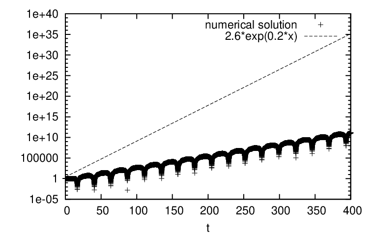
Here ‖b‖[0,∞)=0.6\|b\|_{[0,\infty)}=0.6, τ=16\tau=16, δ=14\delta=14, take λ=0.2\lambda=0.2. Then a⁡(t)=e−0.2​(15−sin⁡t)​0.2​(2−sin⁡t)+0.2>0.2=αa(t)=e^{-0.2(15-\sin t)}0.2(2-\sin t)+0.2>0.2=\alpha, we evaluate numerically ‖b/a‖[0,∞)<2.6735\|b/a\|_{[0,\infty)}<2.6735. Thus

M2=16e−2.8‖ba‖[0,∞)(0.2+0.6e−0.2⋅14)≈0.61515<1.M_{2}=16e^{-2.8}\left\|\frac{b}{a}\right\|_{[0,\infty)}\left(0.2+0.6e^{-0.2\cdot 14}\right)\approx 0.61515<1.

Then M0<2.6M_{0}<2.6, and we get the estimate |x⁡(t)|<2.6​e0.2​t\displaystyle|x(t)|<2.6e^{0.2t} for the solution of (5.3), see Fig. 2 for the comparison with the absolute value of the numerical solution.

By Remark 6, we get |x⁡(t)|<e0.6​t\displaystyle|x(t)|<e^{0.6t}, which is less sharp for t≥2.389t\geq 2.389.

For the chosen initial conditions, the exponential estimate computed numerically has λ≈0.09\lambda\approx 0.09. However, higher growth rates are possible for the same or even smaller delays and the same coefficient. Let ⌊t⌋\lfloor t\rfloor be the maximal integer not exceeding tt. In the problem

x˙​(t)+0.2​(2−sin⁡t)​x​(h⁡(t))=0,t≥0,x⁡(t)=0,t<0,x⁡(0)=1,h⁡(t)=4​π​⌊t4​π⌋,\dot{x}(t)+0.2(2-\sin t)x(h(t))=0,~t\geq 0,~x(t)=0,~t<0,x(0)=1,~h(t)=4\pi\left\lfloor\frac{t}{4\pi}\right\rfloor, (5.4)

the maximal delay of 4​π4\pi is less than 14. Direct computation implies

x⁡(t)=1−∫0t0.2​(2−sin⁡s)​𝑑s,s∈[0,4​π],x⁡(4​π)=1−0.2​∫04​π(2−sin⁡s)​𝑑s=1−1.6​π<0.x(t)=1-\int_{0}^{t}0.2(2-\sin s)~ds,~s\in[0,4\pi],~~x(4\pi)=1-0.2\int_{0}^{4\pi}(2-\sin s)~ds=1-1.6\pi<0.

Next, x⁡(8​π)=(1−1.6​π)−(1−1.6​π)​1.6​π=(1−1.6​π)2x(8\pi)=(1-1.6\pi)-(1-1.6\pi)1.6\pi=(1-1.6\pi)^{2}, x⁡(4​π​k)=(1−1.6​π)kx(4\pi k)=(1-1.6\pi)^{k}. Here the growth coefficient λ=ln⁡(1.6​π−1)/(4​π)≈0.11\lambda=\ln(1.6\pi-1)/(4\pi)\approx 0.11.

Refer to caption
Figure 2: The absolute value of the solution of (5.3) with x⁡(0)=1x(0)=1, ϕ⁡(t)=0\phi(t)=0 compared to the theoretical estimate from Theorem 3. The scale in xx is logarithmic.

For both (5.2) and (5.3), Theorem 3 gives an estimate with a lower exponent than Remark 6.

Finally, consider an example with oscillating coefficients.

Example 4.

For the equation

x˙​(t)+0.2​(0.5−sin⁡(t))​x​(t−2−sin⁡t6)+0.2​(0.5+sin⁡(t))​x​(t−2−sin⁡t12)=0,t≥0,\dot{x}(t)+0.2(0.5-\sin(t))x\left(t-\frac{2-\sin t}{6}\right)+0.2(0.5+\sin(t))x\left(t-\frac{2-\sin t}{12}\right)=0,~t\geq 0, (5.5)

we have τ1=0.5\tau_{1}=0.5, τ2=0.25\tau_{2}=0.25, ‖b1‖[0,∞)=‖b2‖[0,∞)=0.3\|b_{1}\|_{[0,\infty)}=\|b_{2}\|_{[0,\infty)}=0.3. Take λ=0.02\lambda=0.02, then we estimate numerically that

a⁡(t)≥α≈0.18,‖b1/a‖[0,∞)<1.691,‖b2/a‖[0,∞)<1.669,a(t)\geq\alpha\approx 0.18,~\|b_{1}/a\|_{[0,\infty)}<1.691,~\|b_{2}/a\|_{[0,\infty)}<1.669,

in (4.2) we have

M1<(0.02+0.3​e0.01+0.3​e0.005)​(0.5​e0.01⋅1.691+0.25​e0.005⋅1.669)<0.7953,M_{1}<\left(0.02+0.3e^{0.01}+0.3e^{0.005}\right)\left(0.5e^{0.01}\cdot 1.691+0.25e^{0.005}\cdot 1.669\right)<0.7953,

and M0<4.89M_{0}<4.89, thus for x⁡(0)=1x(0)=1, ϕ⁡(t)≡0\phi(t)\equiv 0, the solution of (5.5) satisfies

|x⁡(t)|≤4.89​e−0.02​t.|x(t)|\leq 4.89e^{-0.02t}. (5.6)
Remark 7.

Inequality (5.6) implies that equation (5.5) with two oscillating coefficients is uniformly exponentially stable. We do not know other stability tests for this class of equations.

6 Conclusions and Discussion

As we mentioned in Introduction, there are several related topics, in particular, asymptotic integration or obtaining asymptotic formulas for solutions of a given equation. Such asymptotic expressions of the form x⁡(t)=(C+o⁡(1))​eα​t\displaystyle x(t)=(C+o(1))e^{\alpha t} have been constructed for various classes of differential equations: scalar and vector, linear and nonlinear, equations with concentrated and distributed delays, including integro-differential equations. The review paper [3] includes a detailed outline of these results with historical notes. Asymptotic formulas give a good approximation for long time behavior of solutions, but are useless for finite intervals. Estimates obtained in the present paper apply to finite intervals, and constitute a natural addition to asymptotic formulas. Most papers on asymptotic integration consider specific classes of equations, such as equations with a dominating non-delay term, autonomous equations, equations with a single delay. We have considered scalar equations with several variable delays and measurable coefficients. Another advantage of our results is an explicit form for these estimates, which we illustrated by examples of different types.

When investigating asymptotic stability, most authors considered equations with positive coefficients. If both positive and negative coefficients were involved, it was usually assumed that a positive part dominates over the negative one, see, for example, [4, 6, 7, 9, 16, 18, 22]. In Theorem 1, we got uniform exponential stability conditions, when the equation contains several delays, and all the coefficients may be oscillatory, see Example 5.5. We suggest that in this case, not only the estimate, but also the stability test is new.

Assume that bkb_{k} in Theorem 2 are proportional. Then (4.6) leads to the following uniform exponential stability condition

0≤bk(t)≤βk,lim inft→∞∑k=1mbk(t)>0,t−τk≤hk(t)≤t,k=1,…,m,∑k=1mbkτk<10\leq b_{k}(t)\leq\beta_{k},~\liminf_{t\rightarrow\infty}\sum_{k=1}^{m}b_{k}(t)>0,~t-\tau_{k}\leq h_{k}(t)\leq t,~k=1,\dots,m,~\sum_{k=1}^{m}b_{k}\tau_{k}<1 (6.1)

for (2.1), and to a relevant estimate of solutions. Note that for (2.1) with several variable delays and coefficients, one in the right-hand side of (6.1) is the best possible constant [22].

Let us state possible extensions of the results of the present paper.

  1. 1.

    Obtain explicit estimates of solutions for nonlinear equations in general, and for specific cases, for example, models of population dynamics. These include, but not limited to, the Hutchinson, the Mackey-Glass and the Nicholson blowflies equations.

  2. 2.

    Extend the estimates to a vector DDE. Consider other types of delay, such as distributed, as well as equations of the second and higher order, and stochastic differential equations.

  3. 3.

    In this paper, we presented pointwise estimates. It would be interesting to obtain estimates in an integral form.

  4. 4.

    For the case of a single delay

    x˙​(t)+b⁡(t)​x​(h⁡(t))=f⁡(t),b⁡(t)≥b0>0,t−h⁡(t)≤τ,\dot{x}(t)+b(t)x(h(t))=f(t),~~b(t)\geq b_{0}>0,t-h(t)\leq\tau,

    we obtain estimates for ‖b‖​τ<1\|b\|\tau<1. Relax this condition, replacing 11 with either 32\frac{3}{2} or a sharp constant in (1,1.5)(1,1.5).

Acknowledgment

The second author acknowledges the support of NSERC, the grant RGPIN-2015-05976. Both authors are grateful to the reviewer for valuable comments and suggestions.

References

  • [1] R.  Agarwal, L. Berezansky, E. Braverman, A. Domoshnitsky, Nonoscillation Theory of Functional Differential Equations with Applications, Springer, New York, 2012.
  • [2] J. A. D. Appleby and D. D. Patterson, Subexponential growth rates in functional differential equations, Discrete Contin. Dyn. Syst. 2015, Dynamical systems, differential equations and applications. 10th AIMS Conference. Suppl., 56–65.
  • [3] J. A. D. Appleby and D. D. Patterson, Hartman-Wintner growth results for sublinear functional differential equations, Electron. J. Differential Equations 2017 (2017), Paper No. 21, 45 pp.
  • [4] N. V. Azbelev and P. M. Simonov, Stability of Differential Equations with Aftereffect. Stability and Control: Theory, Methods and Applications, 20. Taylor &\& Francis, London, 2003.
  • [5] L. Barreira and C. Valls, A Perron-type theorem for nonautonomous delay equations, Cent. Eur. J. Math. 11(7) (2013) ,1283–1295.
  • [6] L. Berezansky and E. Braverman, On exponential stability of linear differential equations with several delays, J. Math. Anal. Appl. 324 (2006), 1336–1355.
  • [7] L. Berezansky and E. Braverman, Explicit stability conditions for linear differential equations with several delays, J. Math. Anal. Appl. 332 (2007), 246–264.
  • [8] L. Berezansky and E. Braverman, Nonoscillation and exponential stability of delay differential equations with oscillating coefficients, J. Dyn. Control Syst. 15 (2009), 63–82.
  • [9] L. Berezansky and E. Braverman, New stability conditions for linear differential equations with several delays, Abstr. Appl. Anal. 2011, Art. ID 178568, 19 pp.
  • [10] J. Diblík, Asymptotic representation of solutions of equation y˙​(t)=β⁡(t)​[y⁡(t)−y⁡(τ⁡(t))]\dot{y}(t)=\beta(t)[y(t)-y(\tau(t))], J. Math. Anal. Appl. 217 (1998), 200–215.
  • [11] J. Diblík, Long-time behaviour of solutions of delayed-type linear differential equations, Electron. J. Qual. Theory Differ. Equ. 2018, Paper No. 47, 23 pp.
  • [12] A. Domoshnitsky, M. Gitman and R. Shklyar, Stability and estimate of solution to uncertain neutral delay systems, Bound. Value Probl. 2014, 2014:55, 14 pp.
  • [13] E. Fridman, Introduction to Time-Delay Systems. Analysis and Control. Systems &\& Control: Foundations &\& Applications, Birkhäuser/Springer, Cham, 2014.
  • [14] M. Gil’, Stability of Vector Differential Delay Equations. Frontiers in Mathematics, Birkhäuser &\& Springer Basel AG, Basel, 2013.
  • [15] K. Gu, V. L. Kharitonov and J. Chen, Stability of Time-delay Systems, Control Engineering, Birkhäuser Boston, Inc., Boston, MA, 2003.
  • [16] S. A. Gusarenko and A. I. Domoshnitsky, Asymptotic and oscillation properties of first-order linear scalar functional-differential equations, Differential Equations 25, 1989, 1480–1491.
  • [17] I. Győri, F. Hartung and J. Turi, Preservation of stability in delay equations under delay perturbations, J. Math. Anal. Appl. 220 (1998), 290–312.
  • [18] I. Győri and F. Hartung, Stability in delay perturbed differential and difference equations, Topics in functional differential and difference equations (Lisbon, 1999), Fields Inst. Commun., 29, Amer. Math. Soc., Providence, RI, 2001, 181–194.
  • [19] I. Győri and L. Horváth, Sharp estimation for the solutions of inhomogeneous delay differential and Halanay-type inequalities, Electron. J. Qual. Theory Differ. Equ. 2018, Paper No. 54, 18 pp.
  • [20] V. L. Kharitonov and D. Hinrichsen, Exponential estimates for time delay systems, Systems Control Lett. 53 (2004), 395–405.
  • [21] V. Kolmanovskii and A. Myshkis, Introduction to the Theory and Applications of Functional-Differential Equations, Mathematics and its Applications, 463, Kluwer Academic Publishers, Dordrecht, 1999.
  • [22] T. Krisztin, On stability properties for one-dimensional functional-differential equations, Funkcial. Ekvac. 34 (1991), 241–256.
  • [23] Ch. G. Philos and I. K. Purnaras, On the behavior of the solutions for certain first order linear autonomous functional differential equations, Rocky Mountain J. Math. 36 (2006), 1999–2019.
  • [24] M. Pinto and J. Collardo, Asymptotic integration of nonautonomous delay-differential systems, J. Math. Anal. Appl. 199 (1996), 654–675.
  • [25] M. Pituk, A Perron type theorem for positive solutions of functional differential equations, Electron. J. Qual. Theory Differ. Equ. 2018, Paper No. 57, 11 pp.
  • [26] J. W. H. So, J. S. Yu and M. P. Chen, Asymptotic stability for scalar delay differential equations, Funkcial. Ekvac. 39 (1996), 1–17.
  • [27] S. G. Xu, J. Lam and M. Y. Zhong, New exponential estimates for time-delay systems, IEEE Trans. Automat. Control 51 (2006), 1501–1505.
  • [28] T. Yoneyama and J. Sugie, On the stability region of scalar delay-differential equations, J. Math. Anal. Appl. 134 (1988), 408–425.