Solving Vehicle Routing Problem Using Quantum Approximate Optimization Algorithm
Abstract
In this paper, we describe the usage of the Quantum Approximate Optimization Algorithm (QAOA), which is a quantum-classical heuristic, to solve a combinatorial optimization and integer programming task known as Vehicle Routing Problem (VRP). We outline the Ising formulation for VRP and present a detailed procedure to solve VRP by minimizing its simulated Ising Hamiltonian using the IBM Qiskit platform. Here, we attempt to find solutions for the VRP problems: , , and , where each (n, k) represents a VRP problem with locations and vehicles. We find that the performance of QAOA is not just dependent upon the classical optimizer used, the number of steps p in which an adiabatic path is realized, or the way parameters are initialized, but also on the problem instance itself.
Keywords:
Ising Model, Combinatorial Optimization, Variational Quantum AlgorithmsI Introduction
A majority of the real world applications involve mapping the task at hand to an optimization problem, whose solutions are either fully known or can be approximated by relaxing some of its constraints. In general, the increment in problem size or augmentation of additional constraints can increase the hardness of the problem. This means that the computational resources required in solving them scale-up exponentially, making them computationally intractable. Hence, researchers worldwide have been working on developing efficient tools and techniques for solving these problems efficiently with the available computing power.
With the recent development of quantum processors by IBM bib_IBM, Rigetti bib_Pyquil, Google bib_Google etc, various proposals have been made to use them to find solutions for optimization problems. In general, quantum computing devices are supposed to have a computational advantage over classical processors by using quantum resources such as superposition and entanglement. However, the computational capabilities of these current generation quantum processors also known as Noisy Intermediate-Scale Quantum (NISQ) bib_Preskill devices, are considerably restricted due to their intermediate size (in terms of qubits count), limited connectivity, imperfect qubit-control, short coherence time and minimal error-correction. Hence, they are only able to run algorithms with limited circuit depth. The Quantum Approximate Optimization Algorithm (QAOA) bib_Farhi is one of such algorithm which belongs to the class of quantum-classical hybrid variational algorithms. It can be thought of as a coarsely trotterized adiabatic time evolution in steps to i.e., the ground state of a Hamiltonian which encodes the problem from i.e., the ground state of the Hamiltonian which is known and easier to prepare. Thus, it can be used to solve combinatorial optimization problems mapped to the minimization of an Ising Hamiltonian on near-term devices. As the Ising problem is itself NP-hard, QAOA is an expected candidate for demonstrating quantum supremacy. Here, in this paper, we use QAOA to solve the Vehicle Routing Problem (VRP), which is an NP-hard combinatorial optimization problem bib_Feld.
Structure – In Section II, we discuss VRP and present its Ising formulation in Section III. Then, in Section IV, we explain QAOA in detail and present our simulation results in Section V. Finally, in Section VI, we discuss the performance and limitations of using QAOA to solve combinatorial optimizations problem in general.
II Vehicle Routing Problem
Vehicle Routing Problem is an NP-hard combinatorial optimization problem. Any problem instance of VRP involves vehicles, and locations (other than the depot ). Its solution is the set of routes in which all of the vehicles begin and end in the , such that each location is visited exactly once. The optimal route is the one in which the total distance travelled by vehicles is least. In a way, this problem is a generalization of the classic Travelling Salesman Problem bib_TSP_Bik, where now a group of salesmen begin and end at the same location while having to collectively serve locations such that each location is served exactly once.
In most real world applications, the VRP problem bib_VRP_Bik is generally augmented by constraints, such as vehicle capacity or limited coverage-time. However, here we only focus on showing how to solve the most basic version of VRP without any of these additional constraints.
III Ising Formulation of VRP
To solve a problem instance of VRP using QAOA, we first need to map it to the minimization of an Ising Hamiltonian bib_Lucas. We do this by first finding the , which encodes the given problem instance.
Let be the binary decision variable which has the value if there exists an edge from to with weight , else it is . To represent a solution to VRP problem, there will be decision variables. Next, we for every edge we define two sets and . The set will contain the nodes to which node sends an edge. Similarly, the set will contain all the nodes which send an edge to node . Hence, the VRP can be forumalted as
| (1) |
Subjected to the following constraints:
| (2) |
| (3) |
| (4) |
| (5) |
Here, Eqs. (2), (3) impose the node-visiting constraint so that each node is visited exactly once. Also, the Eqs. (4), (5) impose the constraint to enforce that all the vehicles begin from and return back to depot , i.e., the node . Now, using Eqs. (1-5), the energy functional of the above problem can be written as:
| (6) |
| (7) |
| (8) |
| (9) |
| (10) |
| (11) |
Here, is a constant, which is dependent on the problem instance itself. Next, for , we can represent all the decision variables using the following vector :
| (12) |
Using , we also define the following vectors for every node : and . The first vector is with , if , . Similarly, the second vector is with , if , . These two additional vectors could be understood more clearly using the following two Eqs. (13-14):
| (13) |
| (14) |
From Eq. (12), we can represent minimization of as a quadratic unconstrained binary optimization (QUBO) problem which is isomorphic to the ising problem. In general, a QUBO problem for a graph may be defined as:
| (15) |
Here the quadratic coefficient represents the edge weight i.e., coupling or interaction between two nodes, the linear coefficient represents the node weight i.e., contribution from individual nodes, and the term is a constant offset. In order to find these coefficient in the QUBO forumations bib_DWAVE of given in Eq. (6) we first put in Eqs. (13-14) in Eqs. (8-9) respectively, then expand and regroup Eq. (6) according to Eq. (15).
| (16) |
From Eq. (16), we get the coefficients Q , g and c:
| (17) |
| (18) |
| (19) |
Here, is a vector with first elements and rest elements , vector is with if , , else and is a weight vector. From this, to construct Ising Hamiltonian for we expand Eq. (15) by using Eqs. (17-19) and rewrite all the binary variables using spin variables .
| (20) |
By regrouping bib_DWAVE together similar terms from the expansion, one can express for as:
| (21) |
| (22) |
| (23) |
| (24) |
Replacing with i.e. the Pauli-Z operator acting on qubit, gives the quantum mechanical description of which is implementable on a quantum computer.
IV Quantum Approximate Optimization Algorithm
Adiabatic quantum computation (AQC)bib_Albash was the first quantum computation model to be used for solving hard combinatorial optimization problems. Unlike the gate-based quantum computation model, it was based on adiabatic theorem from quantum mechanics. In this model, to perform any computation we need two Hamiltonians called and . Amongst them, the ground state of should be an easily preparable state such as and ground state of encode the solution to our problem. Both Hamiltonians and , should be local, i.e. they only involve terms for interactions between a constant number of particles. The instantaneous Hamiltonian for the system is:
| (25) |
In AQC, , i.e., the difference between the ground state and first excited state energy of bounds the step size one can take to follow adiabatic pathway bib_Ahar. Hence, the computation time to solve any problem rises exponentially as becomes infinitesimally small. This limits its capability to solve a certain instance of hard optimization problems.
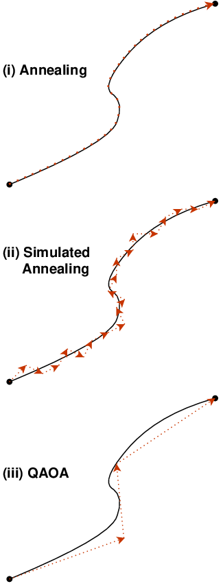
In Quantum Approximate Optimization Algorithm (QAOA), we eliminate this restriction on the step size. Instead, whole of the adiabatic pathway is discretized in some steps, where represents precision (Fig. 1). To do this, we trotterize the unitary into steps using the parameters as follows:
| (26) |

In gate-model quantum computation this means bib_Ahar that starting from some initial product state , we apply a parameterized gate sequence to produce the state . For some optimal value of the parameters: , this is the ground state of . The parameters are provided by a classical processor, and also optimized by a classical optimization routine based on the result of energy measurement for final state . Hence, QAOA belongs to the class of hybrid quantum-classical variational algorithms.
V Simulations and Results
We have executed QAOA using IBM Qiskit to solve VRP for three problem instances: , , and , where each represents a problem with locations and vehicles with a distance matrix representing the squared euclidean distances between locations. One needs qubits to encode the problem instance, i.e., state of each qubit represents the possibility of an edge between two nodes. The mixing Hamiltonian and the cost Hamiltonian for this problem are:
| (27) |
| (28) |
In , we have terms of , terms of , and is an offset. In each of the following cases, we begin with the state , which is the ground state of given in Eq. (27). This state is prepared by applying Hadamard on all qubits initialized to . From Eq. (26), this state is evolved as:
| (29) |
For the evolved state , we calculate energy by measuring the expectation value of as:
| (30) |
Running a classical optimization routine on Eq. (30), we get the optimal value of as . To get the final result we measure the state . As shown in Fig. (2), the state can collapse to any of the possibilities. To visualize the solution, we represent the index of the collapsed state as length bit string which represents flattened version of the adjacency matrix of the graph.
V.1 Experiment 1
In the first experiment, we have solved the problem instance , described by the following distance matrix:
| (31) |


To encode the problem, we used qubits. Using COBYLA optimizer, for we were able to get the correct solution with sufficient probability. In Fig. (2), we have shown the probability distribution of our result for . States corresponding to indexes and are equiprobable and solution states. We present the visualization of the state indexed in Fig. (4) using the following adjacency matrix :
| (32) |
The cost in both cases come out to be .
V.2 Experiment 2
In the second experiment, we have solved the problem instance , described by the following distance matrix:
| (33) |

To encode the problem, we used qubits. We tried COBYLA, NELDER MEAD, and L-BFGS-B optimizers, for different values of ranging from to . Fig. (5) represents the visualization of the state indexed: , i.e., the state we got, using the following adjacency matrix :
| (34) |

The cost in this case comes out to be .
Where as, Fig. (6) represents the visualization of the state indexed:
, i.e., the optimal state we should have got, using the following adjacency matrix :
| (35) |
The cost in this case comes out to be . Therefore, as shown in Fig. (5), the solution we got was not the optimal one i.e., given in Fig. .
V.3 Experiment 3
In the third experiment, we have solved the problem instance , described by the following distance matrix:
| (36) |
To encode the problem, we used qubits. Using COBYLA optimizer, for we were able to get the correct solution with sufficient probability. In Fig. (3), we have shown the probability distribution of our result for for top 12 feasible solutions. States corresponding to indexes and are equiprobable and solution states.
We present the visualization of the state in Fig. (7) using the following adjacency matrix :
| (37) |

The cost in both cases come out to be .
VI Discussions
Here, we have used Quantum Approximate Optimization Algorithm to solve the Vehicle Routing Problem. In past, QAOA has been widely used in solving various combinatorial hard optimization problems bib_Wang; bib_Gutmann; bib_Cedric. However, looking at the results from Exp. (V.1), (V.2), and (V.3), we conclude that in general, for a finite value of , there is no guarantee that the solution achieved by QAOA corresponds to the most optimal solution of the original combinatorial optimization problem bib_Will. This is because, in QAOA instead of the following the adiabatic time evolution path, we try to guess it using steps. So, the first straightforward reason could be that the chosen value does not produce a good enough guess. Then, another reason which could explain failure of QAOA at larger values of , could be the emergence of new local minimums in our solution energy-landscape which traps both gradient-free and gradient-based optimizers, and make them converge prematurely.
Moreover, in the previous studies bib_Will; bib_Alam; bib_Guerr, it has been shown that while running QAOA on near term quantum processors, noise-based errors affect both the fidelity of state: , prepared by a quantum routine, and the minimized expectation value of , i.e., . Characterizing the behaviour of noisy quantum hardware is essential in developing error correction code, and noise-resilient algorithms. Therefore, in future, we would like to do a noise analysis of QAOA for solving the problem of VRP with additional constraints, or any other combinatorial optimization problem.
Data Availability
The code created to run these simulations and related supplementary data could be made available to any reader upon reasonable request.
Acknowledgments
U. would like to thank IISER Kolkata and Bikash’s Quantum (OPC) Pvt. Ltd. for providing hospitality during the course of the project work. B.K.B. acknowledges the support of Institute fellowship provided by IISER Kolkata.
References
- (1)
- (2) Qiskit: An Open-source Framework for Quantum Computing, 10.5281/zenodo.2562110 (2019).
- (3) R. Smith, M. J. Curtis, and W. J. Zeng, A Practical Quantum Instruction Set Architecture, arXiv:1608.03355 [quant-ph] (2016).
- (4) Google AI Quantum Lab. Retrieved December 16, 2019, from https://research.google/teams/applied-science/quantum/.
- (5) J. Preskill, Quantum Computing in the NISQ era and beyond, Quantum 2, 79 (2018).
- (6) E. Farhi, J. Goldstone, and S. Gutmann, A Quantum Approximate Optimization Algorithm, arXiv:1411.4028 [quant-ph] (2014).
- (7) S. Feld, C. Roch, T. Gabor, C. Seidel, F. Neukart, I. Galter, W. Mauerer, and C. Linnhoff-Popien, A Hybrid Solution Method for the Capacitated Vehicle Routing Problem Using a Quantum Annealer, Front. ICT 6, 13 (2019).
- (8) K. Srinivasan, S. Satyajit, B. K. Behera, and P. K. Panigrahi, Efficient quantum algorithm for solving travelling salesman problem: An IBM quantum experience, arXiv:1805.10928 [quant-ph] (2018).
- (9) A. Nowbagh, B. K. Behera, and P. K. Panigrah, A Quantum Approach for Solving Vehicle Routing Problem: An IBM Quantum Experience, DOI:10.13140/RG.2.2.18975.30887 (2019).
- (10) A. Lucas, Ising formulations of many NP problems, Front. Phys. 2, 5 (2014).
- (11) D-Wave Systems: Difference between BQM, Ising, and QUBO problems? Retrieved December 16, 2019, from https://support.dwavesys.com/hc/en-us/community/posts/360017439853-Difference-between-BQM-Ising-and-QUBO-problems.
- (12) G. Verdon, M. Broughton, and J. Biamonte, A quantum algorithm to train neural networks using low-depth circuits, arxiv:1712.05304 [quant-ph] (2019)
- (13) T. Albash, and D. A. Lidar, Adiabatic Quantum Computing, Rev. Mod. Phys. 90, 015002 (2018).
- (14) D. Aharonov, W. V. Dam, J. Kempe, Z. Landau, S. Lloyd, and O. Regev, Adiabatic Quantum Computation is Equivalent to Standard Quantum Computation. 45th Annual IEEE Symposium on Foundations of Computer Science (2004).
- (15) Z. Wang, S. Hadfield, Z. Jiang, and E. G. Rieffel, Quantum approximate optimization algorithm for MaxCut: A fermionic view, Phys. Rev. A 97, 1-13 (2018)
- (16) E. Farhi, J. Goldstone, and S. Gutmann, A Quantum Approximate Optimization Algorithm Applied to a Bounded Occurrence Constraint Problem, arXiv:1411.4028 [quant-ph] (2014).
- (17) C. Lin, and Y. Zhu, Performance of QAOA on Typical Instances of Constraint Satisfaction Problems with Bounded Degree. arXiv:1601.01744 [quant-ph]. (2016).
- (18) M. Willsch, D. Willsch, F. Jin, H. D. Raedt, and K. Michielsen, Benchmarking the Quantum Approximate Optimization Algorithm, arxiv:1907.02359 [quant-ph] (2019).
- (19) M. Alam, A. Ash-Saki, and S. Ghosh, Analysis of Quantum Approximate Optimization Algorithm under Realistic Noise in Superconducting Qubits, arxiv:1907.09631 [quant-ph] (2019).
- (20) G. Guerreschi, and A. Y. Matsuura, QAOA for Max-Cut requires hundreds of qubits for quantum speed-up, Sci. Rep. 9, 6903 (2019).