Experimental adaptive Bayesian estimation of multiple phases with limited data
Abstract
Achieving ultimate bounds in estimation processes is the main objective of quantum metrology. In this context, several problems require measurement of multiple parameters by employing only a limited amount of resources. To this end, adaptive protocols, exploiting additional control parameters, provide a tool to optimize the performance of a quantum sensor to work in such limited data regime. Finding the optimal strategies to tune the control parameters during the estimation process is a non-trivial problem, and machine learning techniques are a natural solution to address such task. Here, we investigate and implement experimentally for the first time an adaptive Bayesian multiparameter estimation technique tailored to reach optimal performances with very limited data. We employ a compact and flexible integrated photonic circuit, fabricated by femtosecond laser writing, which allows to implement different strategies with high degree of control. The obtained results show that adaptive strategies can become a viable approach for realistic sensors working with a limited amount of resources.
Quantum sensing devices are among the most promising quantum technologies. Their implementation relies on the use of quantum probes to attain enhanced performances in the estimation of one or more parameters compared to classical ones. Quantum metrology aims at identifying the best strategy able to provide this quantum advantage Giovannetti et al. 2004; Giovannetti et al. 2006; Paris 2009; Schnabel et al. 2010; Giovannetti et al. 2011; Pezzè et al. 2018; Pirandola et al. 2018. This is achieved by carefully tailoring the probe state, the interaction, and the measurement, in order to extract the information on the relevant parameter, and by the optimal choice of the estimator through data post-processing Gianani et al. 2019. When performing a single parameter estimation, the optimal strategy is unequivocally identified through the saturation of the Cramér-Rao bound (CRB), which establishes the maximum achievable precision on the measured parameter Helstrom 1976. The CRB is asymptotically saturated with the number of resources employed to probe the system during the measurement. Conversely, the realisation of quantum sensors, able to perform estimations in realistic scenarios, poses two constraints to sensing devices: the resources to be used for probing are limited, and systems can show high complexity, often involving more than one parameter. Due to the finite number of available resources, it becomes of paramount importance to optimize the estimation protocols in order to reach the sought accuracy bounds employing the smallest number of resources possible. Such problem has been explored recently with several theoretical analysis. A possible approach towards the protocol optimization is that of exploiting adaptive strategies. These have been successfully employed in single-parameter estimation Berry and Wiseman 2000; Armen et al. 2002; Wheatley et al. 2010; Higgins et al. 2007; Berni et al. 2015; Paesani et al. 2018; Rubio and Dunningham 2019a; Lumino et al. 2018; Daryanoosh et al. 2018. In this regard, machine learning (ML) approaches have provided a significant speed up in the saturation of the ultimate bounds Hentschel and Sanders 2009; Lovett et al. 2013; Lumino et al. 2018; Palittapongarnpim et al. 2017.
On the other hand, measuring multiple parameters at once might be necessary in complex systems characterized by a set of parameters, where a time or spatial dependency can prevent the successful realization of subsequent single-parameter estimations. The parameters considered can span from multiple phases Polino et al. 2019; Humphreys et al. 2013a; Pezzè et al. 2017, to phase and phase diffusion in frequency-resolved phase measurements Genoni et al. 2012; Vidrighin et al. 2014; Altorio et al. 2015, and phase and loss in absorbing systems Albarelli et al. 2019a. In other instances where a system depends solely on one parameter, a multiparameter approach could still be favourable as other parameters can be interrogated as a control to monitor the quality of the sensor itself Roccia et al. 2018; Cimini et al. 2019a; Cimini et al. 2019b. In general, the saturable bounds for quantum multiparameter strategies are not as defined as in the single parameter case, and trade-offs in the achievable precision for each of the parameters have to be sought Albarelli et al. 2019b; Ragy et al. 2016; Szczykulska et al. 2016; Nichols et al. 2018; Gessner et al. 2019.
In this context, it becomes of paramount importance to identify both a suitable estimation scenario and a corresponding platform for an experimental investigation of adaptive multiparameter estimation protocols. A notable scenario to investigate is multiphase estimation Macchiavello 2003; Humphreys et al. 2013b; Ballester 2004; Liu et al. 2016; Gagatsos et al. 2016; Pezzè et al. 2017; Ge et al. 2018; Ciampini et al. 2016; Gessner et al. 2018; Gatto et al. 2019; Guo et al. 2019; Polino et al. 2019. Not only such scenario provides a benchmark for multiparameter quantum metrology, but it has a plethora of practical applications in quantum imaging Szczykulska et al. 2016; Albarelli et al. 2019b. A fundamental step is to find a suitable experimental platform to realize multiphase estimation. A viable solution is provided by integrated photonics, which enables the implementation of complex circuits with reconfiguration capabilities Carolan et al. 2015; Orieux and Diamanti 2016; Wang et al. 2018; Atzeni et al. 2018; Taballione et al. 2019; Wang et al. 2019 with applications ranging from quantum simulation, to computation, and communication. This platform represents a promising system for optical quantum metrology, since interferometers with several embedded phases can be employed as a benchmark platform to study multiparameter estimation problems. In this direction, first results on multiphase estimation with quantum input probes have been recently reported Polino et al. 2019, using a three-arm interferometer fabricated by femtosecond laser writing Della Valle et al. 2008; Gattass and Mazur 2008. Here, we report on multiphase estimation experiments performed with an integrated platform using different adaptive protocols. We identify the strategy providing better performances in terms of optimal estimation and computational resources. In particular, we have experimentally tested the proposed approach by feeding with single-photon states an integrated three-mode interferometer realized by the femtosecond laser writing technique. The employed technique is a Bayesian learning protocol which exploits advantages of Montecarlo approach, such as its independence of integration space dimensions Granade et al. 2012. This solution seems to be ideal for adaptive multiparameter problems, where complex optimizations could involve multiple integrations. Here we employ experimentally for the first time an adaptive strategy optimized in the limited data regime for multiphase estimation. Using this algorithm, we demonstrate that the convergence to the CRB can be experimentally achieved after only few photons. Importantly, such convergence is achieved for both the simultaneously estimated phases. Our results improve research for identifying optimal learning strategy and finding experimental platforms suitable to test multiparameter estimation problems also in the limited data regime.
Results
Bayesian multiparameter estimation
In multiparameter estimation, the aim is to measure simultaneously an unknown set of parameters by reaching the maximum precision allowed by the amount of resources employed in the process. In general, the set of parameters is encoded within the evolution of a system, either described through a unitary operator or a more general map . The value of the unknown parameters can be estimated by preparing a suitable probe state and sending it to evolve throughout the system. Information on the unknown parameters can be retrieved by measuring the output state with a set of measurement operators , where represents the set of possible outcomes. Such process is then repeated times to improve precision in the estimation process. After probes have been prepared and measured, the obtained sequence of measurement outcomes has to be converted in a set of parameters estimates through a suitably chosen function . A possible choice of estimator is provided by Bayesian protocols. This class of estimators is based on encoding the initial knowledge on the parameters in a probability function , called prior distribution, which is updated according to the Bayes rule at each step of the estimation protocol. The posterior distribution after probes reads , where is the likelihood function of the system expressing the conditional probability of obtaining the measurement sequence for given values of the parameters , and is a normalization constant. Then, the mean of the posterior distribution can be exploited as the estimate of the unknown parameters . Bayesian protocols present several important properties. In particular, it can be shown that such approach is asymptotically unbiased, meaning that the estimated values converge to the true values when is large enough. This is related to the quadratic loss , whose average value over all measurement sequences is commonly employed as a figure of merit to quantify the convergence of the estimation process. The coefficients can be chosen to reflect different weights between the parameters, while for equally relevant parameters they can be set as . Hereafter, we will consider this latter scenario and thus define the quadratic loss as . Furthermore, in a Bayesian framework the posterior distribution also provides a confidence region for the parameters estimates, which is represented by the covariance matrix of . This latter figure of merit is obtained for each single estimation experiment composed of a sequence of probes, and has no counterpart in frequentist approaches Li et al. 2019. In general, Bayesian bounds for both the quadratic loss and the covariance matrix depend on the amount of a priori knowledge available Li et al. 2019; Rubio et al. 2018; Rubio and Dunningham 2019a; Rubio and Dunningham 2019b. Asymptotically for large values of , corresponding to the regime where the amount of information acquired in the estimation process far exceeds the a priori knowledge, the covariance matrix satisfies the Cramér-Rao inequality , where is the Fisher information matrix Liu et al. 2019 and thus corresponds to its inverse. Such quantity also provides an asymptotic bound for the quadratic loss as .
Adaptive protocols can be employed when, besides the set of unknown parameters , the user has access to an additional set of control parameters that can be changed throughout the estimation process. More specifically, after each of the probes is sent and measured, the acquired knowledge is employed to change the values of for the next probe to maximize the extraction of information in the subsequent measurement. Within a Bayesian framework, such knowledge is encoded in the posterior distribution. Hence, after each step of the estimation protocol, the user can decide the values of the control parameters starting from (see Fig. 1a). Adaptive protocols represent a relevant tool in phase estimation process. Indeed, the adoption of adaptive strategies becomes a crucial requirement even in the single-parameter case to optimize the algorithm performances Wiseman 1995; Berry and Wiseman 2000; Armen et al. 2002; Hentschel and Sanders 2009; Wheatley et al. 2010; Granade et al. 2012; Lovett et al. 2013; Wiebe and Granade 2016; Paesani et al. 2018; Lumino et al. 2018, with the aim of achieving the ultimate bounds provided by the Cramér-Rao inequality for small values of Lumino et al. 2018. Furthermore, in more complex systems characterized by a phase-dependent Fisher information matrix, adaptive strategies become crucial to reach equal performances for all values of the unknown parameter(s) Cimini et al. 2019b.
Adaptive protocols for multiarm interferometers
Given the general scenario described in the previous section, it is crucial to identify and test experimentally protocols to saturate the ultimate bounds with a very limited number of probes. In this context, multiarm interferometers represent a benchmark platform to perform simultaneous estimation of multiple phases. The platform is schematically shown in Fig. 1b, and represents the -mode generalization of a Mach-Zehnder interferometer in the multimode regime Spagnolo et al. 2012; Chaboyer et al. 2015; Ciampini et al. 2016; Polino et al. 2019. More specifically, it is composed by a sequence of a first multiport splitter, employed to prepare the probe state, a series of phase shifts between all the optical modes, and a second multiport splitter which defines the output measurement. Both multiport splitters can be in principle designed according to appropriate decompositions Reck et al. 1994; Clements et al. 2016 to implement any linear unitary transformation. The internal phase shifts can be divided in two layers. The first one corresponds to the unknown parameters to be measured, while the second one takes the role of the control parameters for adaptive estimation; we note that in our implementation the number of controls . Here, is the number of independent parameters, since one of the phases is considered as the reference mode. Both the unknown parameters and the control ones contribute to the overall phase differences within the interferometer.
We study different adaptive protocols for Bayesian learning of the unknown phases of this platform injected by a single-photon state, by focusing both theoretically and experimentally on the three-mode scenario () with two independent parameters (). More specifically, we choose both for state preparation and state measurement transformation a balanced tritter described by unitary matrix with Spagnolo et al. 2013. Injecting a single photon on input port corresponds to generating a sequence of probe states of the form , which represents a single-photon state exiting in the balanced superposition of the three modes. The Fisher information matrix in this scenario shows a phase-dependent profile , meaning that without adaptive strategies the asymptotic precision will be different depending on the actual phase values. In particular, by looking at the inverse of , we obtain , which is obtained for six different phase pairs . For those pairs, minimum asymptotic quadratic loss is achieved.
Bayesian protocols require in general expensive computational resources, due to the need of evaluating complex integrals to determine the normalization constant , as well as the estimated values and their corresponding covariance matrices. A possible solution is to perform a discretization of the parameters space, thus converting integrals to sums. In this case, the bin size has to be chosen depending on the minimum error expected at the end of the estimation process. However, such solution becomes quickly unmanageable when the number of parameter increases, since such discretization has to be performed in a -dimensional space. A different solution has been explored in Granade et al. 2012 for Bayesian learning problems by using a Sequential Monte Carlo (SMC) approach. Indeed, Monte Carlo methods seems to be a natural solution, due to their capability of reaching convergence independently from the integration space dimension. The SMC method approximates the infinite dimensional support with a finite number of elements , called particles, with associated probability weights . The error in the approximation can be arbitrarily reduced by increasing the number of particles, leading to a trade-off between computational time and accuracy of the approximation. In the context of Bayesian analysis, any distribution in the particles approximation is expressed as .
We now consider the case of an initial prior knowledge corresponding to a uniform distribution. In the particles scenario, this prior information is approximated by a set of randomly drawn pair of phases with equal weights to satisfy the normalization condition . During the experiment, the information about the unknown phases is updated according to the Bayes rule after each measurement outcome . In the particle approximation, having fixed control phases, this corresponds to updating the particle weights as , while keeping the particles unchanged. The estimation of is then provided by the expectation value of the posterior distribution . As discussed in Granade et al. 2012, the particle approximation needs some additional steps to avoid the introduction of further errors throughout the estimation process. In particular, after a few iterations the non-zero weights will be mostly concentrated on a small subset of , reducing the validity of the approximation. To avoid such effect, it is possible to employ resampling techniques Liu and West 2012. More specifically, when the particle weights become too concentrated according to a given threshold condition, a new set of particles is generated by adding a small random perturbation to the original particles (see Supplementary information IA for more details). The weights are then reset to , and the estimation process restarts. Within this framework, we now have to define the adaptive rule to determine the value of the control parameters at each step depending on the actual knowledge. More specifically, at each step of the estimation process one has to decide the control parameters (here, the additional phases ) for the next probe. To this end, we consider different strategies.
A first approach (i) is based on choosing the control phases according to , where . This strategy looks to set the interferometer phases to those values leading to a minimum bound for according to the Cramér-Rao inequality. While this approach is tailored to work in the asymptotic regime of large , its performances are not guaranteed to be optimal for small . An upside of this approach is that setting the control parameters does not require complex optimization steps, since an analytic rule can be easily defined.
In order to devise a strategy working in the small regime, one can consider a second strategy (ii) which is specifically tailored to work for all values of . To this end, we adapted the protocol described in Granade et al. 2012 to the multiparameter scenario implemented by our system. By this approach, the choice of the control phases is performed to optimize a given figure of merit, known as utility function (). Canonical choices for are information gain or quadratic loss. In our case, we choose . Hence, at each step the minimization algorithm finds the best control phases that, averaged over all possible measurement outcomes, leads to a minimum value for the sum of the parameters confidence intervals. This is thoroughly discussed in Sec. IB of the Supplementary Information. Given that this method relies on numerical optimization steps, it is more expensive in terms of computational resources than the previous strategy based on the Fisher information matrix. Conversely, it provides the advantage of searching the optimal control phases for all values of , thus covering the limited data regime where asymptotic approaches may not be the proper choice.
We have then performed numerical simulations to characterize the performances of the two algorithms. More specifically, we have sampled random pairs of phases in the interval . For each pair, we simulated estimation processes where single-photon probes are sent in the interferometer. The results are shown in Fig. 2. We first tested the performances of both algorithms (i) and (ii). We observe that, concerning strategy (i), the protocol fails to approach the Cramér-Rao bound even for . This is related to the periodicity of the likelihood function, which presents multiple equivalent points. Approach (i) seeks for setting the phase differences to a fixed point, and it is not able to resolve such periodicity issue. Better results are obtained by applying at each step a random (but known) set of control phases (iii), which shows better convergence while not reaching the Cramér-Rao bound. However, the application of this strategy is capable of resolving the multiple periodicity. One can then consider a modified version (i’) of the asymptotic protocol (i), where the first control phases are drawn from a uniform distribution, while for the strategy works as (i). Numerical evidence shows that the best choice for this parameter is . We observe that, with this modified strategy, the Cramér-Rao bound is approached for . Better results are obtained with the optimized strategy (ii), in particular in the small regime. For , we observe that both strategies (i’) and (ii) provide similar performances since the experiment progressively approaches a large scenario where the Fisher information matrix defines the system sensitivity. In this work we experimentally implement the optimal strategy to guarantee a faster convergence of the estimation process.
Integrated circuit for multiphase estimation
The platform employed in this experiment is an integrated three-arm interferometer. This system has been employed in Ref. Polino et al. 2019 for the simultaneous estimation of two relative phase shifts between the arms of a three mode interferometer (Fig. 3). We first discuss the circuit layout and parameters, while we subsequently describe the working condition used for the multiphase estimation experiments reported below.
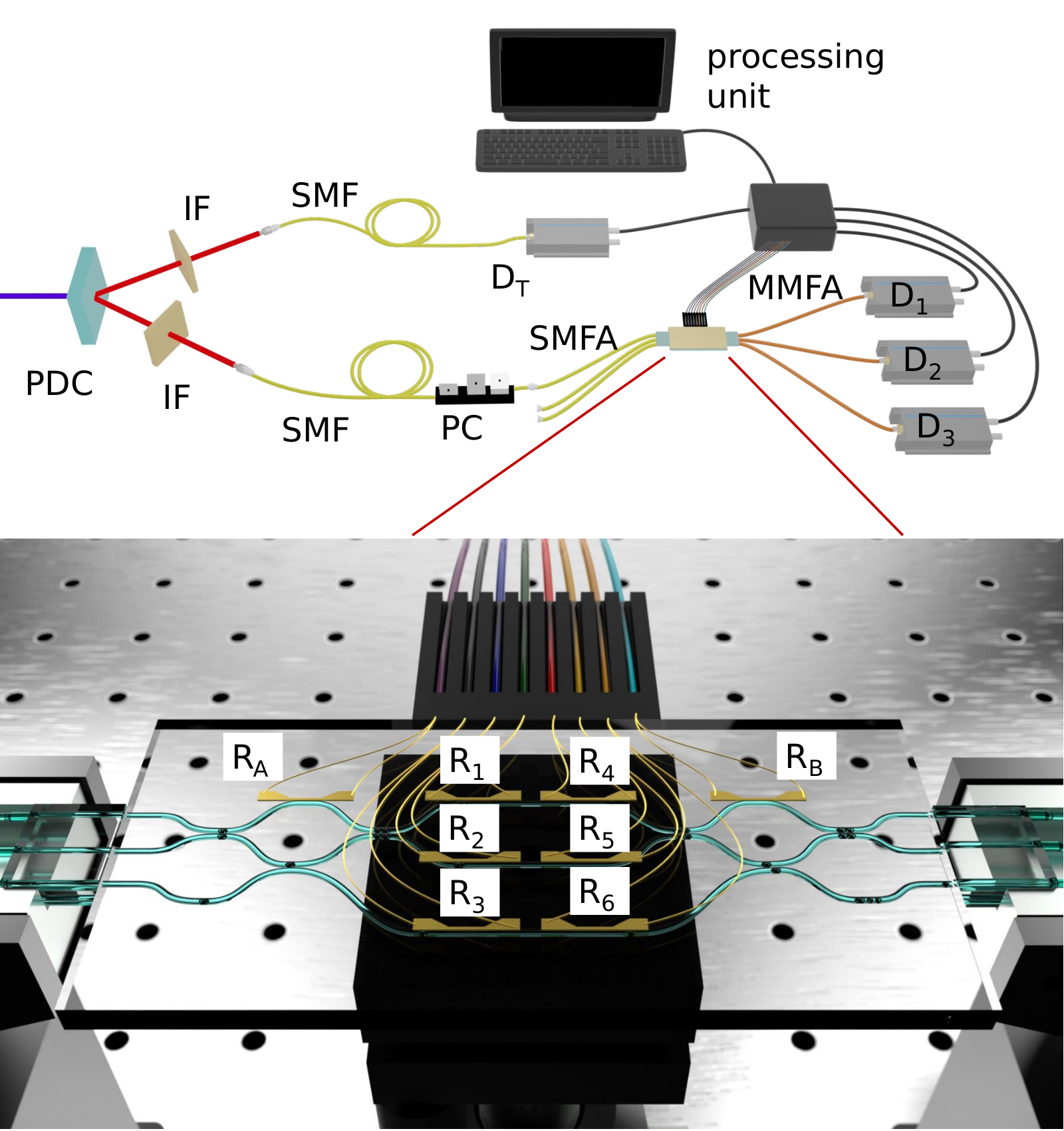
The platform is a three-arm interferometer realized in a glass chip through femtosecond laser writing Della Valle et al. 2008; Gattass and Mazur 2008. The interferometer, optimized for operation at nm, is implemented by two cascaded tritters (three-mode beam splitters) and interspersed with phase shifters. Each tritter is decomposed in a 2-D planar configuration Reck et al. 1994 consisting of three balanced directional couplers and one phase shifter () for tritter (). These phase shifters, as well as those placed between the two tritters, can be tuned by means of the thermo-optic effect, using microresistors that are patterned in a thin gold layer covering the chip surface. When an electrical current is applied to the resistor, an optical path change on the waveguide is induced by the dissipated heat Flamini et al. 2015. In particular, let us consider the dissipated power on resistor subjected to a current , where we also include that the value of the resistor depends on the current due to its temperature change. The two induced relative phase shifts between the arms of the interferometer with respect to the reference mode, have the following general dependence on the dissipated powers:
| (1) |
where and stands for the static phases of the interferometer. Parameters and are the linear and quadratic response coefficients relative to the dissipated power , respectively, while represent the nonlinear coefficients associated to the product of the two powers and to include cross-talk effects. In our device 8 independent resistors are present (Fig. 3). Resistors and are exploited to tune tritter phases and , respectively. Conversely, resistors , along mode 1, , along mode 2 and , along mode 3, are employed to tune the internal relative phase shifts of the interferometer, according to (1). The operations of tritters and are described through the unitary evolutions and , respectively, while the action of each phase shifter along mode is described through a unitary matrix (). The overall evolution of the interferometer is given by .
In order to characterize the relevant parameters necessary to fully describe the evolution of the interferometer, we measure the output probabilities when single photons are injected along input 1, tuning the current applied on each resistor. The probabilities have been theoretically modeled by modifying the ideal expression with additional terms, taking into account non-ideal visibilities and dark counts of the detectors. In this way, we performed an overall fit of all the measured probabilities to determine the 58 chip parameters (Supplementary Information II) and finely reconstruct the likelihood probability of our system.
According to the scheme of Fig. 1b, the unknown phases to be estimated are the pairs (), relative to the chosen reference arm . The 8 resistors allow us to finely tune and control all the relevant phase shifts of the interferometer. The tritters phases can be tuned and are chosen in order to maximize the sensitivity of the interferometer. Using single photon probes, the optimal configuration for our interferometer employs mode 1 as input and mode 2 as reference. In this case, the trace of the inverse of Fisher Information matrix, minimized over all possible internal phases, is . The unknown phases are tuned by means of resistors and , according to (1), while the control phases are tuned by resistors and (see Methods).
Experimental adaptive multiphase estimation
We perform the experiment by continuously adapting the present tunable circuit following the optimized Bayesian-SMC method [strategy (ii)]. This allows us to achieve best attainable estimation with a limited number of resources. The probes are heralded single photons at nm generated by a degenerate type-II SPDC process inside a BBO crystal, pumped by a pulsed nm laser. A photon from each pair is sent through the circuit, entering in input 1, and acts as probe, while the other photon acts as the trigger for the heralding process (see Fig. 3). An event is then recorded as the coincidence between the trigger detector and one of the three outputs of the circuit. The interaction of the probe with the chip operator encodes information about onto its state. Finally, the result of the measurement is collected and used to identify the optimal settings for the next experimental step.

The phases to be estimated can be chosen by setting the currents flowing in three resistors (see Methods). In order to test the protocol over different estimation experiments, we have identified pair of phases uniformly distributed (Fig. 4). Resistors are used to tune the control phases necessary for the adaptive strategy. After the first event, where currents are chosen at random, we implement strategy (ii): optimal control phases are calculated by minimizing the expected posterior variance. The nearest available control currents , limited by the precision of our power supply (Keithley 2230), are calculated and effective control phases are applied to the device. The calculation of the prior distribution for each step is made through the particle approximation. A uniform grid of pairs of phases (Fig. 5a) is assumed as initial set for the prior distribution. This choice is performed yo avoid any possible harmful periodicity during the estimation process. Examples of prior information evolution during an experiment are reported in Fig. 5b-d. In Fig. 5 c the resampling step is shown, where particles with zero weight of the previous step (Fig. 5b) are rearranged in more significant locations (see Sec. IA of Supplementary Information for more details). Each pair is estimated times, adopting resources (photons) as for the numerical simulations discussed above. Single experiments are reported in details in Sec. II of Supplementary information. Algorithm performances are shown in Fig. 6. A first evaluation consists in averaging the experimental quadratic loss for each pair of phases over all independent runs. As a result, the overall quadratic loss saturates the CRB with a limited number of resources, in agreement with the numerical simulations described above. Furthermore, saturation occurs both for off- and diagonal matrix elements of the CRB. In particular, the latter show that the CRB is reached with similar performances in the estimation of both phases. This result is a fundamental feature for multiparameter metrology tasks when both parameters are treated equally. In our case the resulting difference in estimation of the two parameters is less than , when compared to the sensitivity bound. Furthermore, a heuristic estimation of the convergence time to saturate CRB can be calculate by studying the difference . A characteristic time can be computed by using as fit function, with the fitting parameters. The value obtained for is , which underlines the good performance of the adaptive adopted technique in using small number of probes. Another significant property of Bayesian approach is the ability to provide the statistical error in each step of the estimation process, calculated as the variance of the posterior distribution. Final estimated pairs fall on average within the error from true set values of phases (Fig. 4). All these experimental results demonstrate the quality of Bayesian-SMC strategy, confirming it as largely suitable for multiparameter estimation problems. Implementation of this strategy has been enabled onlyby the high reconfigurability of our employed integrated device, which highlights the fundamental role of an appropriate platform for metrology tasks which involve more than one parameter.
Discussion
Multiparameter estimation is a fundamental problem for the realization of realistic quantum sensors in several scenarios. In this task, there are still several open problems and a comprehensive framework has yet to be defined. Hence, it is crucial to identify an experimental platform versatile enough to address different possible approaches. Multiphase estimation provides an ideal scenario with different practical applications. Furthermore, it represents a testbed for different multiparameter estimation protocols. Applying these to real world scenario requires a further step, that is, the optimization of the available resources, so as to attain the minimum reachable uncertainties after a sufficiently small number of measurements. This can be achieved by implementing adaptive strategies.
Here, we have reported the first experimental implementation of a multiphase Bayesian adaptive protocol on an integrated platform, optimized to operate in the limited data regime. We have reviewed different adaptive strategies and selected the one optimizing the cost function given by the trace of the covariance matrix. This has been employed to perform several simultaneous estimations of uniformly distributed pairs of phases. As we have shown, the achievable bounds are attained for both unknown phases after a limited number of probes. Our experiment permits to underline the suitability of such an integrated circuit for performing multiparameter estimation tasks, as well as to exploit the capabilities of the proposed Bayesian adaptive strategy.
This work provides a versatile approach for future perspectives in multiparameter quantum metrology. In particular, these techniques can be directly generalized for multi-photon quantum probes which would provide insight on the achievable quantum accuracy limit. At the same time, the algorithm here described can be applied to more complex integrated platforms, which enable optimized extraction of information. Further perspectives include the study of different multiparameter scenarios, as well as practical applications to quantum sensing of delicate samples Crespi et al. 2012.
Methods
Tuning of circuit parameters for adaptive two-phase estimation
We discuss in more details how we exploit the phases in our interferometer. The pair () represents the unknown phases relative to a reference arm with phase (Fig. 1b). All the relevant phases of the circuit can be finely tuned by means of 8 resistors.
The first step performed aimed at finding the optimal choice for the tritter phases , to maximize the sensitivity of the interferometer. To achieve this goal, we first evaluate the Fisher information matrix associated to the device from the experimentally estimated parameters, Then, we numerically minimize over all possible values of , and internal phases , in the allowed range of dissipated powers (the upper threshold being W, to avoid possible damages to the resistors). We identify such minimum for all combinations of possible inputs and reference arms. The best scenario for our interferometer corresponds to use mode 2 as reference mode and arm 1 as input mode for single photons, with the following values of phases: rad, rad, rad and rad. In this working point, the trace of the inverse of Fisher Information matrix is . We now have to assign each resistor () to tune both the unknown phase shifts , and the control phases for the adaptive algorithms. More specifically, we choose to employ resistors and to tune . Conversely, the control phases are those modified by dissipating power in and . Hence, considering (1) as , we find the following expressions:
| (2) | |||||
| (3) |
with . Note that, in principle, only 4 resistors would be sufficient to tune independently the 4 phase shifts (2 unknown and 2 controls). However, we employed 5 resistors in order to obtain large tunability of the device within limits of the damage threshold of each resistor.
References
- Giovannetti et al. (2004) V. Giovannetti, S. Lloyd, and L. Maccone, Science 306, 1330 (2004).
- Giovannetti et al. (2006) V. Giovannetti, S. Lloyd, and L. Maccone, Physical Review Letters 96, 010401 (2006).
- Paris (2009) M. G. Paris, International Journal of Quantum Information 7, 125 (2009).
- Schnabel et al. (2010) R. Schnabel, N. Mavalvala, D. E. McClelland, and P. K. Lam, Nature communications 1, 121 (2010).
- Giovannetti et al. (2011) V. Giovannetti, S. Lloyd, and L. Maccone, Nature Photonics 5, 222 (2011).
- Pezzè et al. (2018) L. Pezzè, A. Smerzi, M. K. Oberthaler, R. Schmied, and P. Treutlein, Reviews of Modern Physics 90, 035005 (2018).
- Pirandola et al. (2018) S. Pirandola, B. R. Bardhan, T. Gehring, C. Weedbrook, and S. Lloyd, Nature Photonics 12, 724 (2018).
- Gianani et al. (2019) I. Gianani, M. G. Genoni, and M. Barbieri, arXiv preprint arXiv:1909.02313 (2019).
- Helstrom (1976) C. W. Helstrom, Quantum detection and estimation theory (Academic press, 1976).
- Berry and Wiseman (2000) D. Berry and H. Wiseman, Physical review letters 85, 5098 (2000).
- Armen et al. (2002) M. A. Armen, J. K. Au, J. K. Stockton, A. C. Doherty, and H. Mabuchi, Physical Review Letters 89, 133602 (2002).
- Wheatley et al. (2010) T. Wheatley, D. Berry, H. Yonezawa, D. Nakane, H. Arao, D. Pope, T. Ralph, H. Wiseman, A. Furusawa, and E. Huntington, Physical Review Letters 104, 093601 (2010).
- Higgins et al. (2007) B. L. Higgins, D. W. Berry, S. D. Bartlett, H. M. Wiseman, and G. J. Pryde, Nature 450, 393 (2007).
- Berni et al. (2015) A. A. Berni, T. Gehring, B. M. Nielsen, V. Händchen, M. G. Paris, and U. L. Andersen, Nature Photonics 9, 577 (2015).
- Paesani et al. (2018) S. Paesani, A. A. Gentile, J. Santagati, R.and Wang, N. Wiebe, D. P. Tew, J. L. O’Brien, and M. G. Thompson, Physical Review Letters 118, 100503 (2018).
- Rubio and Dunningham (2019a) J. Rubio and J. Dunningham, New Journal of Physics 21, 043037 (2019a).
- Lumino et al. (2018) A. Lumino, E. Polino, A. S. Rab, G. Milani, N. Spagnolo, N. Wiebe, and F. Sciarrino, Physical Review Applied 10, 044033 (2018).
- Daryanoosh et al. (2018) S. Daryanoosh, S. Slussarenko, D. W. Berry, H. M. Wiseman, and G. J. Pryde, Nature Communications 9, 4606 (2018).
- Hentschel and Sanders (2009) A. Hentschel and B. C. Sanders, Physical Review Letters 104, 063603 (2009).
- Lovett et al. (2013) N. B. Lovett, C. Crosnier, M. Perarnau-Llobet, and B. C. Sanders, Physical Review Letters 110, 220501 (2013).
- Palittapongarnpim et al. (2017) P. Palittapongarnpim, P. Wittek, E. Zahedinejad, S. Vedaie, and B. C. Sanders, Neurocomputing 268, 116 (2017).
- Polino et al. (2019) E. Polino, M. Riva, M. Valeri, R. Silvestri, G. Corrielli, A. Crespi, N. Spagnolo, R. Osellame, and F. Sciarrino, Optica 6, 288 (2019).
- Humphreys et al. (2013a) P. C. Humphreys, M. Barbieri, A. Datta, and I. A. Walmsley, Physical Review Letters 111, 070403 (2013a).
- Pezzè et al. (2017) L. Pezzè, M. A. Ciampini, N. Spagnolo, P. C. Humphreys, A. Datta, I. A. Walmsley, M. Barbieri, F. Sciarrino, and A. Smerzi, Physical Review Letters 119, 130504 (2017).
- Genoni et al. (2012) M. G. Genoni, S. Olivares, D. Brivio, S. Cialdi, D. Cipriani, A. Santamato, S. Vezzoli, and M. G. A. Paris, Physical Review A 85, 043817 (2012).
- Vidrighin et al. (2014) M. D. Vidrighin, G. Donati, M. G. Genoni, X.-M. Jin, W. S. Kolthammer, M. S. Kim, A. Datta, M. Barbieri, and I. A. Walmsley, Nature Communications 5, 3532 (2014).
- Altorio et al. (2015) M. Altorio, M. G. Genoni, M. D. Vidrighin, F. Somma, and M. Barbieri, Physical Review A 92, 032114 (2015).
- Albarelli et al. (2019a) F. Albarelli, J. F. Friel, and A. Datta, arXiv preprint arXiv:1906.05724 (2019a).
- Roccia et al. (2018) E. Roccia, V. Cimini, M. Sbroscia, I. Gianani, L. Ruggiero, L. Mancino, M. G. Genoni, M. A. Ricci, and M. Barbieri, Optica 5, 1171 (2018).
- Cimini et al. (2019a) V. Cimini, I. Gianani, L. Ruggiero, T. Gasperi, M. Sbroscia, E. Roccia, D. Tofani, F. Bruni, M. A. Ricci, and M. Barbieri, Physical Review A 99, 053817 (2019a).
- Cimini et al. (2019b) V. Cimini, M. Mellini, G. Rampioni, M. Sbroscia, L. Leoni, M. Barbieri, and I. Gianani, Optics Express 27, 35245 (2019b).
- Albarelli et al. (2019b) F. Albarelli, M. Barbieri, M. G. Genoni, and I. Gianani, arXiv preprint arXiv:1911.12067 (2019b).
- Ragy et al. (2016) S. Ragy, M. Jarzyna, and R. Demkowicz-Dobrzański, Physical Review A 94, 052108 (2016).
- Szczykulska et al. (2016) M. Szczykulska, T. Baumgratz, and A. Datta, Advances in Physics: X 1, 621 (2016).
- Nichols et al. (2018) R. Nichols, P. Liuzzo-Scorpo, P. A. Knott, and G. Adesso, Physical Review A 98, 012114 (2018).
- Gessner et al. (2019) M. Gessner, A. Smerzi, and L. Pezzè, arXiv preprint arXiv:1910.14014 (2019).
- Macchiavello (2003) C. Macchiavello, Physical Review A 67, 062302 (2003).
- Humphreys et al. (2013b) P. C. Humphreys, M. Barbieri, A. Datta, and I. A. Walmsley, Physical review letters 111, 070403 (2013b).
- Ballester (2004) M. A. Ballester, Physical Review A 70, 032310 (2004).
- Liu et al. (2016) J. Liu, X.-M. Lu, Z. Sun, and X. Wang, Journal of Physics A: Mathematical and Theoretical 49, 115302 (2016).
- Gagatsos et al. (2016) C. N. Gagatsos, D. Branford, and A. Datta, Physical Review A 94, 042342 (2016).
- Ge et al. (2018) W. Ge, K. Jacobs, Z. Eldredge, A. V. Gorshkov, and M. Foss-Feig, Physical review letters 121, 043604 (2018).
- Ciampini et al. (2016) M. A. Ciampini, N. Spagnolo, C. Vitelli, L. Pezzè, A. Smerzi, and F. Sciarrino, Scientific Reports 6, 28881 (2016).
- Gessner et al. (2018) M. Gessner, L. Pezzè, and A. Smerzi, Physical Review Letters 121, 130503 (2018).
- Gatto et al. (2019) D. Gatto, P. Facchi, F. A. Narducci, and V. Tamma, Physical Review Research 1, 032024 (2019).
- Guo et al. (2019) X. Guo, C. R. Breum, J. Borregaard, S. Izumi, M. V. Larsen, T. Gehring, M. Christandl, J. S. Neergaard-Nielsen, and U. L. Andersen, Nature Physics (2019).
- Carolan et al. (2015) J. Carolan, C. Harrold, C. Sparrow, E. Martín-López, N. J. Russell, J. W. Silverstone, P. J. Shadbolt, N. Matsuda, M. Oguma, M. Itoh, et al., Science 349, 711 (2015).
- Orieux and Diamanti (2016) A. Orieux and E. Diamanti, Journal of Optics 18, 083002 (2016).
- Wang et al. (2018) J. Wang, S. Paesani, Y. Ding, R. Santagati, P. Skrzypczyk, A. Salavrakos, J. Tura, R. Augusiak, L. Mancinska, D. Bacco, D. Bonneau, J. W. Silverstone, Q. Gong, A. Antonio, K. Rottwitt, L. K. Oxenlowe, J. L. O’Brien, A. Laing, and M. G. Thompson, Science 360, 285 (2018).
- Atzeni et al. (2018) S. Atzeni, A. S. Rab, G. Corrielli, E. Polino, M. Valeri, P. Mataloni, N. Spagnolo, A. Crespi, F. Sciarrino, and R. Osellame, Optica 5, 311 (2018).
- Taballione et al. (2019) C. Taballione, T. A. Wolterink, J. Lugani, A. Eckstein, B. A. Bell, R. Grootjans, I. Visscher, D. Geskus, C. G. Roeloffzen, J. J. Renema, et al., Optics express 27, 26842 (2019).
- Wang et al. (2019) J. Wang, F. Sciarrino, A. Laing, and M. G. Thompson, Nature Photonics (2019).
- Della Valle et al. (2008) G. Della Valle, R. Osellame, and P. Laporta, Journal of Optics A: Pure and Applied Optics 11, 013001 (2008).
- Gattass and Mazur (2008) R. R. Gattass and E. Mazur, Nature Photonics 2, 219 (2008).
- Granade et al. (2012) C. E. Granade, C. Ferrie, N. Wiebe, and D. G. Cory, New Journal of Physics 14, 103013 (2012).
- Li et al. (2019) Y. Li, L. Pezzè, M. Gessner, Z. Ren, W. Li, and A. Smerzi, Entropy 20, 628 (2019).
- Rubio et al. (2018) J. Rubio, P. Knott, and J. Dunningham, Journal of Physics Communications 2, 015027 (2018).
- Rubio and Dunningham (2019b) J. Rubio and J. Dunningham, arXiv preprint arXiv:1906.04123 (2019b).
- Liu et al. (2019) J. Liu, H. Yuan, X.-M. Lu, and X. Wang, Journal of Physics A: Mathematical and Theoretical 53, 023001 (2019).
- Wiseman (1995) H. M. Wiseman, Physical Review Letters 75, 4587 (1995).
- Wiebe and Granade (2016) N. Wiebe and C. E. Granade, Physical Review Letters 117, 010503 (2016).
- Spagnolo et al. (2012) N. Spagnolo, L. Aparo, C. Vitelli, A. Crespi, R. Ramponi, R. Osellame, P. Mataloni, and F. Sciarrino, Scientific Reports 2, 862 (2012).
- Chaboyer et al. (2015) Z. Chaboyer, T. Meany, L. G. Helt, M. J. Withford, and M. J. Steel, Scientific Reports 5, 9601 (2015).
- Reck et al. (1994) M. Reck, A. Zeilinger, H. J. Bernstein, and P. Bertani, Physical Review Letters 73, 58 (1994).
- Clements et al. (2016) W. R. Clements, P. C. Humphreys, B. J. Metcalf, W. S. Kolthammer, and I. A. Walmsley, Optica 3, 1460 (2016).
- Spagnolo et al. (2013) N. Spagnolo, C. Vitelli, L. Aparo, P. Mataloni, F. Sciarrino, A. Crespi, R. Ramponi, and R. Osellame, Nature Communications 4, 1606 (2013).
- Liu and West (2012) J. Liu and M. West, Combined parameter and state estimation in simulation-based filtering (Springer-Verlag, 2012).
- Flamini et al. (2015) F. Flamini, L. Magrini, A. S. Rab, N. Spagnolo, V. D’Ambrosio, P. Mataloni, F. Sciarrino, T. Zandrini, A. Crespi, R. Ramponi, et al., Light: Science & Applications 4, e354 (2015).
- Crespi et al. (2012) A. Crespi, M. Lobino, J. C. Matthews, A. Politi, C. R. Neal, R. Ramponi, R. Osellame, and J. L. O’Brien, Applied Physics Letters 100, 233704 (2012).
Acknowledgments
We acknowledge very fruitful discussions with Nathan Wiebe, and useful discussions with Francesco Hoch on the integrated device calibration. This work is supported by the Amaldi Research Center funded by the Ministero dell’Istruzione dell’Università e della Ricerca (Ministry of Education, University and Research) program “Dipartimento di Eccellenza” (CUP:B81I18001170001), by MIUR via PRIN 2017 (Progetto di Ricerca di Interesse Nazionale): project QUSHIP (2017SRNBRK), by QUANTERA HiPhoP (High dimensional quantum Photonic Platform; grant agreement no. 731473), and by the Regione Lazio programme “Progetti di Gruppi di ricerca” legge Regionale n. 13/2008 (SINFONIA project, prot. n. 85-2017-15200) via LazioInnova spa.