Probing the galactic halo with RR Lyrae stars I: The catalog
Abstract
We present a catalog of 5,290 RR Lyrae stars (RRLs) with metallicities estimated from spectra of the LAMOST Experiment for Galactic Understanding and Exploration (LEGUE) and the Sloan Extension for Galactic Understanding and Exploration (SEGUE) surveys. Nearly 70 per cent of them (3,642 objects) also have systemic radial velocities measured. Given the pulsating nature of RRLs, metallicity estimates are based on spectra of individual exposures, by matching them with the synthetic templates. The systemic radial velocities are measured by fitting the observed velocity as a function of phase assuming an empirical pulsating velocity template curve. Various tests show that our analyses yield metallicities with a typical precision of 0.20 dex and systemic radial velocities with uncertainties ranging from 5 to 21 km s-1 (depending on the number of radial velocity measurements available for a given star). Based on the well calibrated near-infrared or , and -[Fe/H] relations, precise distances are derived for these RRLs. Finally, we include Gaia DR2 proper motions in our catalog. The catalog should be very useful for various Galactic studies, especially of the Galactic halo.
Subject headings
stars: variables: RR Lyrae – Galaxy: abundances– Galaxy: halo– Galaxy: structureI. Introduction
Probing the Galactic structure is an important task to help understand the assemblage history of our Milky Way as well as that of galaxies in general. The Millky Way halo contains some of the oldest stars and structures found in our Galaxy, and thus provides information of the earliest stage of evolution of our Galaxy. Despite its crucial importance, our knowledge of the stellar halo is still far from complete, partly due to the lack of large samples of halo tracers to probe its properties.
Hitherto, the main halo tracers employed include blue horizontal branch (BHB) stars (Xue et al. 2008; Deason et al. 2011; Deason et al. 2014; Das et al. 2016, e.g.), K giants (Xue et al. 2015; Xu et al. 2018, e.g.), near-main-sequence turnoff stars (nMSTO) (Sesar et al. 2011; Pila-Diez et al. 2015, e.g.) and RR Lyrae stars ((Watkins et al. 2009, RRLs; e.g.). The available number of BHB stars is small since they are difficult to identify; distance estimation of K giants is not easy considering that their intrinsic luminosities vary by two orders of magnitude (depending on stellar age and metallicity); and the luminosities of nMSTO are not high enough to be useful for probing the distant outer halo of the Galaxy.
Compared to the other tracers, RRLs are ideal for studying the halo properties. First, RRLs are old (9 Gyr), low-mass metal-poor stars that reside in the instability strip of the horizontal branch (HB) and thus represent a fair sample of the halo populations (Smith 2004). Secondly, their well defined period-luminosity relation makes them good standard candles, allowing one to accurately map out the 3D structure of the halo. Thirdly, they retain a record of the chemical composition of the environment in which they were born, thus can be used to study the early stage chemical evolution of the Galaxy formation. Finally, they are relatively easy to identify based on their colors and variabilities, enabling the construction of samples of few contaminations. In short, RRLs are excellent tracers to study the structure, formation and evolution of the Galactic halo.
Nevertheless, time-domain photometric surveys alone can not provide precise measurements of metallicity and systemic radial velocity of RRLs. Such information has to be extracted from spectroscopic observations. Fortunately, a number of large-scale spectroscopic surveys have been carried out in the past two decades, including the RAVE (Steinmetz et al. 2006), the SDSS/SEGUE (Yanny et al. 2009), the SDSS/APOGEE (Majewski et al. 2017), the LAMOST (Deng et al. 2012; Liu et al. 2014) and the GALAH (De Silva et al. 2015) surveys.
The spectroscopic data, combined with information (e.g. period, phase and amplitude) derived from light curves provided by photometric surveys and astrometric information (e.g. parallax and proper motions) from the Gaia DR2, allow one to construct a large sample of RRLs with full phase space information of 3 dimensional position and velocity, as well as of metallicity, and to use the sample to probe the formation and evolution of the Galactic halo.
Values of metallicity and radial velocity of RRLs can not be measured by treating them as normal, steady stars, as RRLs are pulsating and their spectra vary with time on short time scales. To measure the metallicities of RRLs, the most precise method is to utilize high resolution spectra. High resolution spectroscopy is however quite costly of big telescope time, and no more than a hundred bright local RRLs have been observed this way (For et al. 2011; Kinman et al. 2012; Nemec et al. 2013; Govea et al. 2014; Pancino et al. 2015, e.g.). For low resolution spectra, the traditional method to measure the metallicities of RRLs is the so-called method, first proposed by Preston 1959. The index describes the difference between the spectral types as given by the H i Balmer lines and by the Ca ii K line measured with low-resolution spectra obtained at minimum light. Many studies have been carried out with this method to derive metallicities of RRLs, by calibrating the relation with either spectroscopic or photometric observations (Butler 1975; Freeman et al. 1975; Layden 1994, e.g.). Although this method is efficient, the scale relation between and [Fe/H] show some nonlinear variations in some cases, leading to some random and systemic errors in the final results.
In this paper, we present a new method to measure the metallicities of RRLs. For the modern large-scale spectroscopic surveys (e.g. the LAMOST and SDSS surveys), there are often two to three exposures made per visit, yielding two to three spectra on a short time span. In addition to the multiple spectra from a single visit, some fields are visited more than once. Excluding spectra affected by shock waves, the metallicity can be measured from the individual single-exposure spectra with a template matching technique (see Section 3.1 for detail). The mean value, weighted by the signal-to-noise ratios (SNRs), of estimates yielded by the individual single-exposure spectra, is then adopted as the final metallicity of the RRL.
In addition to metallicity, it is also crucial to precisely measure the systemic radial velocities of RRLs since they are of vital importance for a variety of Galactic studies, such as identifying halo substructures and exploring their origins by kinematics (Vivas et al. 2001; Keller et al. 2008; Miceli et al. 2008; Casetti-Dinescu et al. 2009; Watkins et al. 2009; Carlin et al. 2012, e.g.), and constraining the mass distribution of the Milky Way (Xue et al. 2008; Huang et al. 2016, e.g.).
However, accurately measuring systemic velocities of RRLs is quite challenging since the observed radial velocities contain a pulsation component which, of a typical amplitude of several tens of km s-1, needs to be accounted for. To derive the values of systemic velocity (), two approaches are generally adopted. In one approach, one schedules the observations at the right phase (i.e. ) such that the pulsation has nearly zero contribution to the observed radial velocity, i.e. . This approach is however not suitable for data collected with large scale, multi-object spectroscopic surveys as in our case. Alternatively, one can correct the measured radial velocities for contribution of pulsation assuming a pulsation model (or an empirical template), that describes the pulsation velocity as a function of phase. In this paper, we utilize the latter approach to measure the systemic velocities of RRLs, by adopting the empirical template of radial velocity curves of ab-type RRLs as constructed by Sesar 2012.
The paper is the first one in a series that utilize RRLs to explore the formation and evolution of the Galactic halo. The data used in the current work is described in Section 2. Estimation of metallicities of RRLs from the spectra is introduced in Section 3. Determinations of systemic radial velocities and distances are presented in Sections 4 and 5, respectively. In Section 6, we present the final catalog and describe its general properties. Finally, a summary is given in Section 7.
II. Data
In this Section, we first collect known RRLs identified in the various time-domain photometric surveys or variable source catalogs. Then available spectra are searched for those stars in the various large-scale spectroscopic surveys.
II.1. RR Lyrae stars from photometric surveys
To collect known RRLs, we use the catalogs of variable stars from the QUEST (Vivas et al. 2004; Mateu et al. 2012; Zinn et al. 2014), NSVS (Kinemuchi et al. 2006; Hoffman et al. 2009), LONEOS (Miceli et al. 2008), GCVS (Samus et al. 2009), LINEAR (Sesar et al. 2013) and the Catalina (Drake et al. 2013a; Drake et al. 2014) surveys. Data of the southern Hemisphere are not included since only spectroscopic data in the northern sky are used (see next Section). A prior is set to each survey (see Table 1), according to their observational epochs (higher prior for those surveys more close to the spectroscopic observations described as follows) and the typical number of photometric observations. For each survey, we compile all the available parameters of identified RRLs into a single catalog, including period, amplitude, epoch, mean -band magnitude, variable star type and distance if derived. In total, we obtain a list of 32,243 unique RRLs from those surveys.
Table 1 summarizes the properties of the individual surveys included in the current study. Fig. 1 plots the distributions of the stars in Galactic coordinates, in distances (adopted directly from the literature), in mean band magnitudes and in periods. If a parameter of a given star is available from more than one survey, then the value from the survey with highest prior is adopted.
Finally, we note that the catalogs of Drake et al. 2013b and Drake et al. 2014 do not provide the epochs of maximum light for the catalogued RRLs. For those stars, we have calculated the missing values by ourselves from the light curves provided by the Catalina survey11 1 http://nesssi.cacr.caltech.edu/DataRelease/RRL.html.
| Survey | Filters | Area ( ) | Range of V magnitude | The typical number of | Obsevation year | Sources | Prior | Reference |
|---|---|---|---|---|---|---|---|---|
| photometric observations | ||||||||
| Catalina | 5 | 1 | ||||||
| QUEST | 2 | 2 | ||||||
| NSVS | ROTSE-NT | 0 | 3 | |||||
| LINEAR | no spectra filter | 8,000 | 4 | 4 | ||||
| LONEOS | LONEOS-NT | 0 | 5 | |||||
| SDSS Str82 | 3 | 6 | ||||||
| GCVS | – | – | – | – | – | 1 | 7 |
Notes. The references are: 1– Drake et al. 2013a; Drake et al. 2014 ; 2–Vivas et al. 2004; Mateu et al. 2012; Zinn et al. 2014; 3– Kinemuchi et al. 2006; Hoffman et al. 2009 ; 4–Sesar et al. 2013; 5–Miceli et al. 2008; 6–Watkins et al. 2009; Sesar et al. 2010; Suveges et al. 2012; 7– Samus et al. 2009.

II.2. Spectroscopy
In the current work, our major spectroscopic data set comes from the LAMOST Galactic spectroscopic surveys (Deng et al. 2012; Zhao et al. 2012; Liu et al. 2014). LAMOST (also named Guoshoujing Telescope) is an innovative quasi-meridian reflecting Schmidt telescope capable of simultaneously recording spectra of up to 4000 objects in a large field of view (FoV) of 5 degrees in diameter. The spectra cover the wavelength range from 3700 to 9100 Å with a resolving power . Typically 2 3 exposures are obtained for each plate, with typical integration time per expsystemic velocityosure of 10 to 40 minutes, depending on the brightness of targeted sources. Since the LAMOST FoV is circular, field overlapping cannot be avoided in order to achieve a contiguous sky coverage. About 25 percent of all targets have been observed twice and over 2 percent three times (Yuan et al. 2015). This greatly benefits the measurements of systemic radial velocity of RRLs reported in this work. By June 2016, the LAMOST Galactic surveys, initiated in October 2012, have obtained 6 million quality spectra, mostly of Galactic stars. This number is still increasing at a rate of 1 million per annum.
Another main source of spectra comes from the SDSS/SEGUE (Yanny et al. 2009). As a major component of the SDSS-II, SEGUE operated from 2005 August to 2008 July, and obtained more than 240,000 spectra of Galactic stars of magnitudes , with a spectral coverage and resolution similar to those of LAMOST. In order to obtain spectra of sufficient signal-to-noise ratios (SNRs), the typical total integration time for bright plates of sources of () is 1 hr and that for plates of fainter sources of is 2 hr. The integration time of the individual exposures ranges between 10 30 minutes. SEGUE-2, the successor of SEGUE, obtained additional 155,520 spectra with the same instrument. All the data from SEGUE and SEGUE-II are included in the SDSS Data Release 12 (Alam et al. 2005, SDSS DR12;).
The spectral database of SDSS DR12 is downloaded and then cross-matched with the aforementioned compiled catalog of photometrically identified RRLs. In total, 3,834 common stars are found, with a total of 20,772 single-exposure spectra. Similarly, a total of 3,016 common sources (with a total of 10,667 single-exposure spectra) are found between the photometric catalog of RRLs and the LAMOST DR2 of value-added catalog (Xiang et al. 2015; Xiang et al. 2017). By combining the two data sets, a total of 6,268 RRLs with a total 31,439 single-exposure spectra are obtained. Typical SNRs of those single-exposure spectra are around 15.
III. spectroscopic metallicities
As mentioned, we utilize single-exposure spectra instead of those combined to measure the metallicities, given the pulsating nature of RRLs.
III.1. Measurement method
To estimate the metallicities of RRLs from single-exposure spectra, we adopt a template matching method by comparing the observed spectra with the synthetic ones based on the least- technique. The synthetic spectra library was generated with code SPECTRUM (Gray 1999) of version 2.76, utilizing the Kurucz stellar model atmospheres of Castelli & Kurucz 2004 that cover the wavelength range from 3850 to 5600 Å at a resolution of 2.5 Å. We degrade the model spectral resolution to match that of LAMOST and SDSS (R 1800). Considering the typical ranges of atmospheric parameters of RRLs, we limit our synthetic spectra to parameter ranges: effective temperature 6000 7500 K in step of 100 K, surface gravity 1.5 log 4.0 dex in step of 0.25 dex, and metallicity 3.0 [Fe/H] 0.0 dex in step of 0.1 dex. Considering the old (typically ¿ 9 Gyr) and metal-poor nature of RRLs, we fix the value of -element to iron abundance ratio to 0.4.
In order to more precisely obtain the parameters and [Fe/H], we match the observed spectra with the synthetic ones by two steps. Firstly, we measure the effective temperature by least- fitting. Considering that the Balmer lines are most sensitive to effective temperature, we give twice weights (weighted by the inverse variances of the spectral fluxes) to spectral pixels that cover for , , and lines when comparing the full observed spectra with the synthetic ones of wavelength range from 3850 to 5600 Å pixel by pixel. At this step, effective temperatures are well determined from single exposure spectra.22 2 Surface gravity and metallicity are also estimated at this step but they are not well constrained due to high weights on Balmer lines and thus not been used. The derived effective temperatures are then set as input values at the following second round of fitting. In the second step, values of the Ca ii K line (mostly sensitive to metallicity) and the continum with the synthetic one but fixing to the value deduced in the first step. In this step, spectral pixels covering Caii H and the Balmer lines, i.e. pixels of the wavelength ranges 3960 to 3980, 4092 to 4112, 4330 to 4350 and 4851 to 4925 Å are masked out. Best-fit values of [Fe/H] and log yielded this second round of optimization are adopted for the star. Fig. 2 plots the resulted stellar atmospheric parameters of an RRL as a function of phase. For this particular target, a total of 12 single-exposure spectra are available. We find that the estimated values of and log vary with the phase of pulsation, largely in consistent with the theoretical predictions.
By above two steps, the metallicities of RRLs are obtained from the individual single-exposure spectra. In principle, no matter what the pulsation stage of the RRL is when targeted, its metallicity should unchange and keep the same value. However, due to the effects of shock waves on the hydrogen and metal lines of RRL spectra (Fokin 1992; Gillet & Fokin 2004; Pancino et al. 2015), the estimated [Fe/H] could change significantly depending on the phase when the spectrum was taken. As Fig. 2 shows, the metallicities of an RRLs estimated during phase between 0 and 0.15 vary dramatically, reflecting the significant effects of shock waves during those phases during the pulsation cycle. To avoid the potential bias in the metallicity determinations caused by shock waves, we try to exclude single-exposure spectra possibly affected by the shock effects for parameter estimates. In general, shock waves mostly occur during the phase 0 to 0.15, and 0.85 to 1.0, but they also can happen at other phases. Considering that the Ca ii K line is easily affected by the shock wave effects, here, we adopt its equivalent width (EW) as a criteria to asses whether a spectrum in concern is affected by shock waves or not.
We first calculate the values of equivalent width of the Ca ii K line, EW(Ca ii K), of all model spectra and find the minima for each effective temperature. Then we fit the minima as a function of temperature with a second-order polynomial and find Min[EW(Ca ii K)]=15.62 0.0037 + 2.21. At the same time, we also calculate the EW(Ca ii K) for each of the single-exposure spectra of our sample stars. As Fig. 2 shows, we find that the values of metallicity measured from single-exposure spectra of EW(Ca ii K) less than the corresponding Min[EW(Ca ii K)], are different from those measured at other phases [c.f. Panel (d) of Fig. 2]. This indicates that those former spectra are affected by shock waves and metallicities yielded by those spectra are consequently ignored. The final adopted metallicity and its error are weighted mean by its errors, yielded by single-exposure spectra (see the Section 3.2.1 ), if having metallicity measurement greater than 2. If only one single spectrum available for a star, we directly use the metallicity of this single spectrum as the final adopted value of this star. Finally, we obtain the metallicities for 5,290 RRLs. It should be noted that, Fabrizio et al. 2019 also have estimated the metallicities of 2,382 fundamental RRLs by method very recently.
By comparing the metallicity estimate of common stars selected from LAMOST and SEGUE surveys with similar SNRs (i.e., SNR ), a negligible offset (around 0.04 dex) is found between the metallicity measurements from the spectra obtained by the two surveys. We therefore assume the metallicitiy scales yielded from the two surveys are the same.

III.2. Validation of metallicities
In this Section, we examine the accuracy of metallicities of RRLs measured by above method in the following ways: 1) Check the internal uncertainties using duplicate-observations; 2) Check both the random and systemic errors by comparing with metallicity measurements from high resolution spectroscopy.
III.2.1 Comparison of results from multi-epoch observations
To estimate the internal errors of the metallicities derived, we use multi-epoch observations of our sample stars. Doing so, the differences of two metallicity measurements of similar SNRs (i.e. ) as a function of the mean SNR are shown in Fig. 3. As the figure shows, the median differences are almost zero, with no significant systemic trend. As expected, the standard deviations of the differences decreases with SNR. We fit the standard deviations (divided by ) as a function of SNR, and find . For the observations reported here, the typical standard deviation is about 0.2 dex. We use the standard deviations derived by above function as the error () of the metallicity estimated by individual single-exposure spectrum when it’s SNR less than 40, and for SNR 40, the error are fixed to the value of dex.

III.2.2 Comparison of results with reference stars
In order to check the zero points of our metallicity measurements, we collect reference stars from the literature with reliable metallicity estimates either from high resolution spectroscopy or as a member star of a globular cluster(GC). For GC member stars, we use a compiled catalog of over 3000 variable stars in 103 GCs (Clement 2017). The properties (e.g. metallicities, radial velocities and distances) of those GCs are taken from Harris W. E. 2010. The metallicity scale adopted here is the one established by Carretta et al. 2009, which is a fundamental shift from the older metallicity scale (Zinn & West 1984) with superior abundance analysis methods based on more advanced model atmospheres. In addition, we have collected stars with metallicity and systemic radial velocity estimates measured with high resolution spectroscopy (Clementini et al. 1995; For et al. 2011; Kinman et al. 2012; Nemec et al. 2013; Govea et al. 2014; Pancino et al. 2015, e.g.). We have cross-matched our RRLs spectroscopic sample with above compiled catalogs and obtained 47 stars in common. Those common stars form our reference star sample. Tables 2 and 3 present respectively relevant information of the reference stars, for GC members and from high resolution spectroscopy.
| Cluster | RA (degree) | Dec (degree) | [Fe/H] | RV (km ) | (km ) | Distance (kpc) | |
|---|---|---|---|---|---|---|---|
| NGC 4147 | 182.544 | 18.581 | 1.80 | 183.2 | 0.70 | 19.3 | 1 |
| NGC 5053 | 198.997 | 17.741 | 2.27 | 44.0 | 0.40 | 17.4 | 2 |
| NGC 5024 | 198.359 | 18.162 | 2.10 | 62.9 | 0.30 | 17.9 | 3 |
| NGC 5272 | 205.392 | 28.507 | 1.50 | 147.6 | 0.20 | 10.2 | 11 |
| NGC 5466 | 211.373 | 28.507 | 1.98 | 106.9 | 0.20 | 16.0 | 2 |
| NGC 5904 | 229.827 | 2.283 | 1.29 | 53.2 | 0.40 | 7.5 | 1 |
| NGC 6341 | 259.300 | 43.207 | 2.31 | 120.0 | 0.10 | 8.3 | 1 |
| NGC 7089 | 323.471 | 0.799 | 1.65 | 5.3 | 2.0 | 11.5 | 2 |
| NGC 7078 | 322.580 | 12.316 | 2.37 | 107.0 | 0.20 | 10.4 | 2 |
| Pal 5 | 228.991 | 0.190 | 1.41 | 58.7 | 0.20 | 23.2 | 4 |
| Star | RA (degree) | Dec (degree) | [Fe/H] | Reference | |
|---|---|---|---|---|---|
| DR And | 16.295 | 34.218 | 1.37 | 0.12 | Pancino et al.(2015) |
| BK Eri | 42.483 | 1.420 | 1.72 | 0.21 | Pancino et al.(2015) |
| SZ Gem | 118.431 | 19.273 | 1.65 | 0.07 | Pancino et al.(2015) |
| SS Leo | 173.477 | 0.033 | 1.48 | 0.07 | Pancino et al.(2015) |
| UV Vir | 185.320 | 0.368 | 1.10 | 0.12 | Pancino et al.(2015) |
| UZ CVn | 187.615 | 40.509 | 2.21 | 0.13 | Pancino et al.(2015) |
| RV UMa | 203.325 | 53.988 | 1.20 | 0.08 | Pancino et al.(2015) |
| TW Boo | 221.275 | 41.029 | 1.47 | 0.05 | Pancino et al.(2015) |
| VIII-14 | 256.891 | 58.850 | 2.92 | - | Kinman et al. (2012) |
| V355 Lyr | 283.358 | 43.155 | 1.14 | 0.17 | Nemec et al. (2013) |
| KIC 11125706 | 285.245 | 48.745 | 1.09 | 0.08 | Nemec et al. (2013) |
| NQ Lyr | 286.952 | 42.300 | 1.89 | 0.10 | Nemec et al. (2013) |
| NR Lyr | 287.114 | 38.813 | 2.54 | 0.11 | Nemec et al. (2013) |
| FN Lyr | 287.593 | 42.459 | 1.98 | 0.09 | Nemec et al. (2013) |
| V838 Cyg | 288.516 | 48.200 | 1.01 | 0.10 | Nemec et al. (2013) |
| V1104 Cyg | 289.502 | 50.755 | 1.23 | 0.15 | Nemec et al. (2013) |
| V1107 Cyg | 289.939 | 47.1012 | 1.29 | 0.23 | Nemec et al. (2013) |
| V2470 Cyg | 289.991 | 46.889 | 0.59 | 0.13 | Nemec et al. (2013) |
| V894 Cyg | 293.254 | 46.240 | 1.66 | 0.12 | Nemec et al. (2013) |
As Fig. 4 shows, the values of metallicity estimated in the current work agree well with those of the compiled reference stars, with a negligible offset (0.04) and a standard deviation of 0.22 dex. The dispersion is comparable to that yielded by multi-epoch observations. All the tests manifest that intrinsic consistency of our measurements is good.
In addition, we have also compared the metallicity measurements yielded by the default SEGUE and LAMOST pipelines with the literature values for reference stars. As Fig. 4 shows, both pipelines over estimate the metallicities, sigificantly.

IV. systemic radial velocities
As mentioned in Section I, it is of crucial importance to measure the systemic radial velocities of RRLs. In this Section, we use the empirical template radial velocity curves of RRLs to fit the observed radial velocities as a function of phase as derived from the individual single-exposure spectra of RRLs in order to obtain their systemic radial velocities.
IV.1. Measurement method
Here, we adopt the empirical template radial velocity curves of ab-type RRLs constructed by Sesar 2012 for H, H and H lines. According to Fig. 3 of Sesar 2012, the uncertainty of systemic velocity yielded by fitting the empirical templates increases dramatically for observational phase greater than 0.7. On the other hand, spectra at phases less than 0.1 are liable to strong effects of shock waves. Consequently, we decide to only use single-exposure spectra taken at phases between 0.1 and 0.7. Amongst those, spectra affected by shock waves , as implied by the criteria EW(Ca ii K) ¡ Min[EW(Ca ii K)], are further excluded when deriving the systemic velocity by fitting with the radial velocity template.
For those adopted single-exposure spectrum, we derive the observed RV by fitting , , and line profiles with a Gaussian function, together with a first-order polynomial, and measure their centers (wavelength coverage from 4325 to 4357 Å for line, 4845 to 4878 Å for line and 6548 to 6580 Å for line, are respectively used in the fits.). Considering that we use spectra from two surveys (LAMOST and SDSS), radial velocities derived from spectra of the two surveys need be calibrated to a common scale. Doing so, common sources from the two surveys of similar phases () and high SNRs (¿ 50) are selected, yielding a total of 72 targets. Distributions of the RV differences (LAMOST values minus SDSS ones) for different lines (i.e. , , and ) are shown in Fig. 5. The medians and standard deviations estimated from the distributions are, respectively, , , and km for , , and . We then calibrate LAMOST RVs derived from the three lines to the scales of SDSS, using the median differences found above.
For a given star that has measured at several phases, one can derive the systemic velocity by fitting the following equation,

| (1) |
where is the observational phase, the amplitude of the radial velocity curve, fixed to the mean values reported in Table 1. of Sesar 2012, i.e. 111.9, 90.9 and 82.1 km for , , and respectively, and the radial velocity curve template. If only one radial velocity measurement is available, we directly interpolate the template to get the systemic radial velocity. As an example, Fig. 6 shows the fit for a source with 9 phase data points.
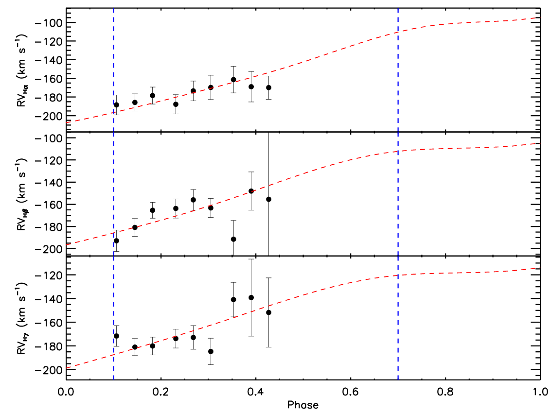
With above procedure, the final systemic radial velocity adopted for a given star is given by the weighted mean (by uncertainties) of measurements yielded by the three Balmer lines, i.e. , and . Basically, the measurement uncertainties are highly dependent on the number of radial velocity measurements used in the fitting.
To derive the random errors of systemic velocity measurements from the individual lines, we solve the following equations:
| (2) |
| (3) |
| (4) |
Here is the number of available radial velocity measurements for a given star and , and are standard deviations of the differences of systemic velocities measured from two out of three lines for given .
Table 4 lists those values for different values of for , , and lines. We compare values of and with those of and obtain mean values of differences 14.59, and 5.83 km for , and , respectively. The non-zero mean RV differences between H, H and H lines are largely due to the existing of a wavelength-dependent residual after the wavelength calibration. We therefore convert and to the scale of by subtracting 14.59 and 5.83 km from the measured values, respectively.
The final value of of a target is calculated by combining results from all three Balmer lines, namely,
| (5) |
| (6) |
| (km ) | (km ) | (km ) | |
|---|---|---|---|
| 1 | 25.19 | 15.81 | 28.81 |
| 2 | 20.17 | 8.57 | 20.46 |
| 3 | 15.25 | 6.57 | 13.85 |
| 12.05 | 5.72 | 10.83 |
We note that the systemic radial velocities of Type c RRLs can also derived, using the template radial velocity curves for Types RRLs, but only the systemic radial velocities of Type ab RRLs are recommended.
IV.2. Validation with reference stars
In order to check the uncertainties (both random and systemic) of our measurements, we collect RRLs from the literature with reliable radial velocity measurements from high-resolution spectroscopy, GC members are also included (Dambis 2009; Harris W. E. 2010; Kinman et al. 2012; Britavskiy 2018). In total, 108 common stars are found and their relevant information is listed in Table. 5 (The information of 29 GC members has been listed in Tables 2). Fig. 7 shows the comparisons. The standard derivations of the differences are 20.6, 14.6, 9.7 and 4.5 km for = 1, 2, 3, and 4, respectively. The median values of the differences are all around 2 km s-1, indicating no significant systemics of our final derived radial velocities. We do not correct such a small offset since it is much smaller than the standard deviations. The results show that once the number of radial velocity measurements available to fit the radial velocity curve is great than 2, the standard deviation of the systemic velocity derived is likely to be less than 10 km . The expected uncertainty drops to only 4.5 km for . This indicate our velocity measurements are quite robust.
Although the pulsation nature of RRLs makes the determinations of their systemic radial velocities more difficult than for other nonpulsating normal stars (Layden 1994; Vivas et al. 2005; Prior et al. 2009, e.g.), the current work shows that one can still use the large numbers of low resolution spectroscopic observations to derive systemic radial velocities with a precisions between 5 and 21 km . This precision is adequate for studying the Galactic halo properties considering that the line-of-sight velocity dispersion of halo stars is around 100 km s-1 (Huang et al. 2016, e.g.).
| Star | RA | Dec | error of | Reference | Star | RA | Dec | error of | Reference | ||
|---|---|---|---|---|---|---|---|---|---|---|---|
| (degree) | (degree) | (km ) | (km ) | – | (degree) | (degree) | (km ) | (km ) | – | ||
| DR Vir | 16.295 | 34.218 | 110.000 | 4.000 | B18 | XX And | 19.364 | 38.951 | 0.000 | 1.000 | D09 |
| CI And | 28.785 | 43.767 | 24.000 | 5.000 | D09 | BK Eri | 42.483 | 1.420 | 141.000 | 10.000 | D09 |
| SS Tau | 54.174 | 5.361 | 11.000 | 10.000 | D09 | TU Per | 47.270 | 53.193 | 314.200 | 0.500 | D09 |
| AR Per | 64.322 | 47.400 | 5.000 | 1.000 | D09 | SZ Vir | 118.431 | 19.273 | 346.000 | 6.000 | B18 |
| RR Gem | 110.390 | 30.883 | 64.000 | 1.000 | D09 | YY Lyn | 116.375 | 37.383 | 93.100 | 15.000 | K12 |
| ZZ Lyn | 117.591 | 37.700 | 147.000 | 15.000 | D09 | VY Lyn | 113.108 | 38.835 | 114.500 | 15.000 | K12 |
| AC Lyn | 118.675 | 38.906 | 25.800 | 15.000 | K12 | VX Lyn | 112.966 | 39.130 | 1.000 | 15.000 | D09 |
| WX Lyn | 113.910 | 39.257 | 26.000 | 15.000 | D09 | TZ Aur | 107.896 | 40.777 | 45.000 | 2.000 | D09 |
| VZ Lyn | 113.170 | 41.627 | 182.100 | 15.000 | K12 | TW Lyn | 116.276 | 43.112 | 39.000 | 1.000 | D09 |
| DD Hya | 123.132 | 2.835 | 156.000 | 1.000 | D09 | AN Cnc | 134.543 | 15.805 | 16.000 | 14.000 | D09 |
| AF Lyn | 128.989 | 41.020 | 121.700 | 15.000 | K12 | P 54-13 | 120.484 | 41.022 | 69.000 | 10.000 | K12 |
| T Sex | 148.369 | 2.057 | 29.000 | 1.000 | D09 | BS 16927 | 146.151 | 41.143 | 70.000 | 10.000 | K12 |
| TT Lyn | 135.784 | 44.586 | 65.000 | 2.000 | D09 | SW Leo | 163.981 | 2.982 | 46.000 | 11.000 | D09 |
| BK UMa | 162.579 | 42.569 | 171.400 | 5.000 | K12 | TV Leo | 167.841 | 5.892 | 96.000 | 5.000 | D09 |
| SS Leo | 173.477 | 0.033 | 163.000 | 2.000 | D09 | SZ Leo | 165.404 | 8.166 | 185.000 | 4.000 | D09 |
| AE Leo | 171.551 | 17.661 | 53.000 | 10.000 | D09 | BN UMa | 169.095 | 41.234 | 19.000 | 10.000 | K12 |
| BQ Vir | 189.114 | 2.426 | 129.000 | 9.000 | D09 | UV Vir | 185.320 | 0.368 | 99.000 | 11.000 | D09 |
| FU Vir | 189.610 | 13.016 | 90.000 | 8.000 | D09 | S Com | 188.190 | 27.029 | 55.000 | 1.000 | D09 |
| DV Com | 190.977 | 28.021 | 136.000 | 10.000 | D09 | EO Com | 194.342 | 28.889 | 72.000 | 10.000 | D09 |
| EM Com | 192.910 | 30.518 | 127.000 | 10.000 | D09 | CD Com | 183.142 | 30.801 | 203.000 | 10.000 | D09 |
| TU Com | 183.446 | 30.985 | 98.000 | 10.000 | D09 | CK UMa | 180.402 | 31.903 | 16.000 | 10.000 | K12 |
| CK Com | 183.711 | 33.102 | 88.000 | 10.000 | D09 | DC CVn | 191.818 | 35.202 | 200.000 | 10.000 | D09 |
| SW Vir | 190.229 | 37.085 | 14.000 | 6.000 | B18 | UZ Vir | 187.615 | 40.509 | 49.000 | 6.000 | B18 |
| Z CVn | 192.439 | 43.774 | 14.000 | 10.000 | D09 | WW Vir | 202.099 | 5.286 | 129.000 | 10.000 | D09 |
| BC Vir | 200.588 | 5.886 | 4.000 | 13.000 | D09 | BB Vir | 207.920 | 6.431 | 38.000 | 13.000 | D09 |
| AV Vir | 200.048 | 9.188 | 153.000 | 1.000 | D09 | UY Boo | 209.693 | 12.952 | 145.000 | 2.000 | D09 |
| ST Com | 199.464 | 20.781 | 68.000 | 10.000 | D09 | RY Com | 196.283 | 23.278 | 31.000 | 8.000 | D09 |
| ST CVn | 209.392 | 29.858 | 129.000 | 1.000 | D09 | EW Com | 198.257 | 31.023 | 19.000 | 10.000 | D09 |
| RZ CVn | 206.263 | 32.655 | 12.000 | 1.000 | D09 | SS CVn | 207.066 | 39.901 | 40.000 | 3.000 | D09 |
| RV Vir | 203.325 | 53.988 | 175.000 | 6.000 | B18 | SX UMa | 201.556 | 56.257 | 154.000 | 1.000 | D09 |
| AE Vir | 216.872 | 3.778 | 208.000 | 10.000 | D09 | RS Boo | 218.389 | 31.755 | 7.000 | 1.000 | D09 |
| TW Vir | 221.275 | 41.029 | 89.000 | 2.000 | B18 | AN Ser | 238.379 | 12.961 | 81.000 | 1.000 | C17 |
| BH Ser | 228.754 | 19.443 | 113.000 | 11.000 | D09 | AW Ser | 241.620 | 15.368 | 126.000 | 15.000 | D09 |
| RW Dra | 248.882 | 57.840 | 112.000 | 1.000 | D09 | V0816 Oph | 265.658 | 4.958 | 28.000 | 10.000 | D09 |
| V0784 Oph | 263.855 | 7.756 | 167.000 | 10.000 | D09 | DL Her | 260.094 | 14.511 | 61.000 | 14.000 | D09 |
| TW Her | 268.630 | 30.410 | 5.000 | 1.000 | D09 | VZ Her | 258.267 | 35.979 | 115.000 | 1.000 | D09 |
| KX Lyr | 278.314 | 40.173 | 36.200 | 0.500 | D09 | SX Aqr | 324.035 | 3.231 | 165.000 | 3.000 | D09 |
| AO Peg | 321.765 | 18.599 | 264.000 | 4.000 | D09 | VV Peg | 333.266 | 18.451 | 34.200 | 0.000 | D09 |
| DZ Peg | 350.029 | 16.069 | 289.500 | 2.400 | D09 | VZ Peg | 355.568 | 24.916 | 264.000 | 1.000 | D09 |
| BK And | 353.775 | 41.103 | 17.000 | 7.000 | D09 |
Notes. The references are: B18– Britavskiy 2018; D09–Dambis 2009; K12– Kinman et al. 2012; C17–Chadid et al. 2017.

IV.3. Discussion
Sesar 2012 shows the amplitude of the template radial velocity curve of RRLs is a function of the amplitude of -band light curve ( AV) . However, only part of the RRLs in our catalog with AV available, we therefore fixed the amplitude of the template radial velocity curve in the fitting to derive the systemic radial velocity (see Section 4.1). To evaluate the effects of our constant radial velocity curve amplitude choice on deriving the systemic radial velocities of RRLs, we re-determine the systemic radial velocities of RRLs with AV known. At this time, we repeat the fitting described in Section 4.1 by using the values of determined by AV from the functions provided by Sesar 2012 and obtain their new systemic radial velocities.
By comparing the new results with our adopted ones, the median velocity difference is found around 2 km s-1 and the standard deviation of the velocity difference is only about 4 km s-1. According to the above test, our constant radial velocity curve amplitude choice show minor effects on deriving the systemic radial velocities of RRLs.
The new values of systemic radial velocity determined in this section is also released in the final catalog for reference.
V. Distances
V.1. Measurement method
Generally, RRLs are divided into three types: Type ab RRLs (RRab) pulsates in the fundamental mode and Type c RRLs (RRc) pulsates in first-overtone mode and Type d RRLs (RRd) pulsates in both modes simultaneously. In our sample, the number of RRd is small, so we do not discuss them separately. Being standard candles, RRLs obey the well-defined relations between absolute visual magnitude and metallicity,
| (7) |
and the near- or mid-infrared period-absolute magnitude-metallicity (),
| (8) |
Coefficients are different for Type ab and Type c RRLs. In this paper, for RRab, coefficients are taken from Muraveva et al. 2018, derived using the latest data of Gaia DR2 (please refer to their Table 4 for more detail). For RRc, coefficients given by Ferro et al. 2017 are used. We adopt the mid-infrared period-absolute magnitude relation provided by Klein et al. 2014,
| (9) |
Compared to the visual - [Fe/H] relation, the near- or mid-infrared relations is less affected by the interstellar extinction. In the following calculations, we prefer distances derived from the near/mid-infrared relations as the final ones.
We cross match our sample with the 2MASS and WISE catalogs to obtain apparent magnitudes in and bands for our sample stars. For sources selected from the Catalina survey, Catalina band magnitudes are converted to Johnson band magnitudes using the transformation equation of Graham et al. 2015, assuming an intrinsic color of 0.2 for RRLs. We then use above relations to obtain the absolute magnitudes and further derive the distances, after the interstellar extinction corrections.
Actually, the WISE magnitudes could been taken as mean magnitudes since they are the mean values typically of 10 single-epoch observations obtained by the WISE survey (Wright et al. 2010). We therefore derive the distances of RRLs from band if uncertainties smaller than 0.1 mag. For only 13 stars without good but band photometry, we derive their distances from band. If both and band photometric uncertainties do not meet our requirements, we use the visual - [Fe/H] relation to obtain the distance.
Totally, we obtain distances for 4,919 RRLs with the above procedures ( 4,061 from band, 13 from band and 845 from band).
V.2. Validation of distances
V.2.1 Comparison with reference stars
In order to check the reliability of our calculations, we firstly compare the distances obtained above with those in the literature for the reference sample, for which the reference distances obtained from the star cluster catalog. As shown in Fig. 8, the average relatives difference () is about 1 per cent, with a dispersion of about 5 per cent. We also collect information of distances from other sources in the literatures (Vivas et al. 2006; Miceli et al. 2008; Watkins et al. 2009; Suveges et al. 2012; Drake et al. 2013a; Drake et al. 2013b; Sesar et al. 2013). The comparison is also shown in Fig. 8. We find that they all agree very well with each other.

V.2.2 Comparison with Gaia parallaxes
We also compare our distances measurements with the Gaia parallaxes. We first convert our distances estimates of uncertainties less than 10 per cent, derived from near- or mid infrared or visual magnitudes, into photometric parallaxes, then compare them with those from the Gaia DR2. Fig. 9 shows the comparison for RRab stars. The mean deviation is mas, consistent with the offset of zero point reported by the Gaia collaboration (Gaia Collaboration 2018). As seen in Fig. 9, four outliers are significantly deviate the one-to-one line. We have checked the distances derived here to those from the literatures and find they are all in great consistent. The reason of those outliers are still unclear and one possible explanation is that their parallax solutions are somehow wrong. Similar results are found for RRc stars.

VI. The final catalog
By combing the SDSS and LAMOST spectroscopic data with literature the photometric data of objects, we have compiled a catalog of RRLs containing 6,268 uniq RRLs. For objects with individual single-exposure SNRs greater than 10 and not affected by shock waves, we measure the metallicities by a least fitting technique. The weighted mean metallicity of the individual spectra, are adopted as the final values. In total, metallicities for 5,290 RRLs are obtained in this way. We then fit the templates of systemic velocity of RRLs provided by Sesar 2012 to the observed ones and derive the systemic radial velocity for 3,642 RRLs. Finally, we use the or - [Fe/H] relations to calculate distances of our sample stars and obtain distance estimates for 4,919 RRLs. All the information derived is compiled into an online catalog containing 6,268 RRLs (Table 6). Table 6 lists the columns contained in the main catalog. Fig. 10 shows the distributions of metallicities, systemic radial velocities, distances and Galactocentric distances of stars in the final, main catalog.
In the near future, we plan to enlarge our sample by including data from additional spectroscopic surveys, e.g., the GALAH survey (De Silva et al. 2015), as well as additional photometrically identified RRLs from the recent time-domain surveys, e.g. the Pan-STARRS1 (Chamber et al. 2016; Sesar et al. 2017); the Gaia DR2 (Clementini et al. 2019). We expect to have precise measurements of metallicities, systemic radial velocities and distances of RRLs for the whole sky. The data shall be very helpful for the study of the formation and evolution of the Galactic halo.
| Column | Unit | Description | |
|---|---|---|---|
| 1 | ID | - | A unique object id for the cataloged RRLs |
| 2 | RA | degree | Right ascension at J2000 from the photometric surveys |
| 3 | DEC | degree | Declination at J2000 from the photometric surveys |
| 4 | GL | degree | Galactic longitude |
| 5 | GB | degree | Galactic latitude |
| 6 | VMAG | mag | -band magnitude |
| 7 | ERR-VMAG | mag | Error in -band magnitude |
| 8 | PER | day | Period |
| 9 | PFROM | - | Reference for period |
| 10 | EPOCH | day | Date of maximum light from the photometric surveys |
| 11 | EPOCH-FLG | - | Which type of EPOCH (MJD,JD, HJD) |
| 12 | VARTYPE | - | Type |
| 13 | SNR | - | Spectral SNR at 4650 Å |
| 14 | FEH-ADOP | dex | Metallicity derived in the current work |
| 15 | ERR-FEH-ADOP | dex | Error of FEH-ADOP |
| 16 | FEH-REF | dex | Metallicity from the literature if available |
| 17 | ERR-FEH-REF | dex | Error of FEH-REF |
| 18 | RV-ADOP 1 | km | Systemic radial velocity derived in the current work |
| 19 | ERR-RV-ADOP | km | Error of RV-ADOP |
| 20 | RV-REF1 | km | Systemic radial velocity determined in Section 4.3 |
| 21 | ERR-RV-REF1 | km | Error of RV-REF1 |
| 22 | RV-REF2 | km | Systemic radial velocity from the literature if available |
| 23 | ERR-RV-REF2 | km | Error of RV-REF2 |
| 24 | DIST-ADOP | kpc | Distance derived in the current work |
| 25 | ERR-DIST-ADOP | kpc | Error of DIST-ADOP |
| 26 | DIST-REF | kpc | Distance from the literature if available |
| 27 | ERR-DIST-ADOP | kpc | Error of DIST-ADOP |
| 28 | PMRA | Proper motion in from Gaia DR2 | |
| 29 | PMDEC | Proper motion in from Gaia DR2 | |
| 30 | ERR-PMRA | Error of the proper motion in from Gaia DR2 | |
| 31 | ERR-PMDEC | Error of the proper motion in from Gaia Dr2 | |
| 32 | NUMBER | – | Number of individual spectra available |
- 1
The radial velocities for type c RRLs are not recommended for use.

VII. Conclusion
We present a catalog of 5,290 RRLs with metallicity estimates. Nearly 70 per cent of them also have systemic radial velocity measurements. We use the single-exposure spectra rather than the combined spectra for metallicity and velocity estimation. We develop a criterion based on the measured equivalent width of Ca ii K line, EW(Ca ii K), to diagnose whether a spectrum is affected by shock waves or not. Those affected are excluded, from the metallicity and velocity estimation.
We measure the systemic radial velocities using the empirical template radial velocity curves of RRLs provided by Sesar 2012 and obtain results for 3,642 RRLs in total. The typical error is about km , dependent on the number of radial velocity measurements available at different phases.
Finally, with the well calibrated near-infrared or , and -[Fe/H] relations, precise distances are derived for 4,919 RRLs.
The results provide vital information to study many issues related to the Galactic halo.
References
- Alam et al. (2005) Alam, S., Albareti, F. D.,Allende P., et al., 2015, ApJS, 219, 12
- Alcock et al. (2003) Alcock, C., Alves, D. R., Becker, A. et al. 2003, ApJ, 598, 597
- Armosky et al. (1994) Armosky, B. J., Sneden, C., Langer, G. E., Kraft, Robert P., 1994, AJ, 108, 1364
- Bai et al. (2015) Bai, Z. R., Zhang, H. t., Zhao, Y. H., et al., 2015, IAUGA, 2251918
- Belokurov et al. (2018) Belokurov, V., Erkal, D., Evans, N. W., et al., 2018, MNRAS, 478, 611
- Butler (1975) Butler, D., 1975, ApJ, 200, 68B
- Britavskiy (2018) Britavskiy, N., Pancino, E., Tsymbal, V., Romano, D., Fossati, L., 2018, MNRAS, 474, 3344
- Brown et al. (2010) Brown, W. R., Geller, M. J., Kenyon, S. J. et al. 2010, AJ, 139, 59
- Cacciari et al. (2005) Cacciari, C., Corwin, T. M., Carney, B. W., 2005, AJ, 129, 267
- Carlin et al. (2012) Carlin, J. L., Majewski, S. R., Casetti-Dinescu, D, I. et al. 2012, ApJ, 744, 25C
- Carretta et al. (2009) Carretta, E., Bragaglia, A., Gratton, R. et al. 2009, å, 508, 695C
- Casetti-Dinescu et al. (2009) Casetti-Dinescu, D. I., Giaard, T. M., Majewski, S. R., et al. 2009, ApJ, 701, 29
- Castelli & Kurucz (2004) Castelli, F., Kurucz, R. L. 2004, astro.ph 5087
- Chaboyer et al. (1999) Chaboyer, B., Green, E. M., Liebert, J., 1999, AJ, 117, 1360
- Chamber et al. (2016) Chambers, K. C., Magnier, E. A., Metcalfe, N., et al. 2016, arXiv:1612.05560
- Chadid et al. (2017) Chadid, M., Sneden, C., Preston, G. W., 2017, ApJ, 835, 187C
- Clementini et al. (1995) Clementini, G., Carretta, E., Gratton, R. et al. 1995, AJ, 110, 2319
- Clement (2017) Clement, C. M., 2017, Vizier Online Data Catalog, 5150
- Clementini et al. (2019) Clementini, G., Ripepi, V., Molinaro, R. et al. 2019, AA, 622A, 60c
- Cohen & Melendez (2005) Cohen, J. G., Meléndez, J., 2005, AJ, 129, 303
- Cui et al. (2012) Cui, X. Q., Zhao, Y. H., Chu, Y. Q. et al. 2012, Research in Astronomy and Astrophysics, 12, 1197
- Das et al. (2016) Das P., Williams A., Binney J., 2016, MNRAS, 463, 3169
- Dambis (2009) Dambis, A. K., 2009, MNRAS, 396, 553
- Deason et al. (2011) Deason, A. J., Belekurov, V., Evans, N. W., et al., 2011, MNRAS, 416, 2903
- Deason et al. (2014) Deason, A. J., Belekurov, V., Koposov, S. E.,et al., 2014, ApJ, 787, 30
- Deng et al. (2012) Deng, L. C., Newberg, H. J., Liu, C. et al., 2012, Research in Astronomy and Astrophysics, 12, 735
- De Silva et al. (2015) De Silva, G. M., Freeman, K. C., Bland-Hawthorn, J., et al., 2015, MNRAS, 449, 2604
- Drake et al. (2013a) Drake, A. J., Catelan, M., Djorgovski, S. G. et al. 2013, ApJ, 765, 154
- Drake et al. (2013b) Drake, A. J., Catelan, M., Djorgovski, S. G. et al. 2013, ApJ, 763, 32D
- Drake et al. (2014) Drake, A. J., Graham, M. J., Djorgovski, S. G. et al. 2014, ApJS, 213, 9D
- Fabrizio et al. (2019) Fabrizio, M., Bono, G., Braga, V. F. et al. 2019, ApJ, 883L, 31C
- Ferro et al. (2017) Ferro, A. A., Bramich, D. M., Giridhar, S. 2017, RMxAA, 53, 121
- For et al. (2011) For, B. Q., Sneden, C., Preston, G. W., 2011, ApJS, 197, 29
- Fokin (1992) Fokin, A. B., 1992, MNRAS, 256, 26F
- Freeman et al. (1975) Freeman, K. C., Rodgers, A. W., 1975, ApJ, 201L, 71F
- Fusi et al. (1996) Fusi Pecci F., Buonanno R., Cacciari C. et al. 1996, AJ, 112, 1461
- Gaia Collaboration (2016) Gaia Collaboration, Brown, A. G. A., Vallenari, A., et al. 2016, AA, 595, A2
- Gaia Collaboration (2018) Gaia Collaboration, Helmi, A., van Leeuwen, F., et al. 2018, AA, 616, A12
- Gillet & Fokin (2004) Gillet, D., Fokin, A. B. 2004, AA, 565, 73
- Govea et al. (2014) Govea, J., Gomez, T., Preston, G. W. et al. 2014, ApJ, 782, 59
- Gray (1999) Gray, R. O. 1999, ascl.soft 10002G
- Graham et al. (2015) Graham, M. J., Diorgovski, S. G., Stern, D., et al. 2015, Nature, 518, 74
- Harris W. E. (2010) Harris, W. E. 2010, arXiv:1012.3224
- Hoffman et al. (2009) Hoffman, D. I., Harrison, T. E., McNamara, B. J. 2009, AJ, 138, 466
- Huang et al. (2016) Huang, Y., Liu, X. W., Yuan, H. B., et al. 2016, MNRAS, 463, 2623
- Keller et al. (2008) Keller, S. C., Murphy, S., Prior, S. et al, 2008, ApJ, 678, 851
- Klein et al. (2014) Klein, C. R., Richards, J. W., Butler, N. R., Bloom, J. S., 2014, MNRAS, 440, 96
- Kinemuchi et al. (2006) Kinemuchi, K., Smith, H. A., Woniak, P. R. et al. 2006, AJ, 132, 1202K
- Kinman et al. (2012) Kinman, T. D., Cacciari, C., Bragaglia, A. et al. 2012, MNRAS, 422, 2116
- Kraft et al. (1992) Kraft, R. P., Sneden, C., Langer, G. E., Prosser, Charles F., 1992, AJ, 104, 645
- Layden (1994) Layden, A. C., 1994, AJ, 108, 1016L
- Liu et al. (2014) Liu, X. W. et al., 2014, Vol. 298, IAU Symposium, Feltzing S., Zhao G., Walton N. A., Whitelock P., eds., pp. 310321
- Majewski et al. (2003) Majewski, S. R., Skrutskie, M. F., Weinberg, M. D., Ostheimer, J. C., 2003, ApJ, 599, 1082
- Majewski et al. (2010) Majewski, S. R., Wilson, J. C., Hearty, F. et al. IAUS, 265, 480
- Majewski et al. (2017) Majewski, S. R., Schiavon, R. P., Frinchaboy, P. M., et al., 2017, AJ, 154, 94
- Mateu et al. (2012) Mateu C., Vivas A. K., Downes J. J. et al 2012, ApJ, 427, 3374
- Miceli et al. (2008) Miceli, A., Rest, A., Stubbs, C. W. et al. 2008, ApJ, 678, 865
- Muraveva et al. (2018) Muraveva, T., Delgado, H. E., Clementini, G. et al. 2018, MNRAS, 481, 1195
- Nemec et al. (2013) Nemec, J. M., Cohen, J. G., Ripepi, V. et al. 2013, ApJ, 773,181
- Pancino et al. (2015) Pancino, E., Britavskiy, N., Romano, D. et al. 2015, MNRAS, 447, 2404
- Pila-Diez et al. (2015) Pila-Diez, B., de Jong, J. T. A., Kuijken, K. et al., 2015, AA, 579, 38
- Pojmanski (2002) Pojmanski, G. 2002, AcA, 52, 397
- Preston (1959) Preston, G. W., 1959, ApJ, 130, 507
- Prior et al. (2009) Prior, S. L., Da Costa, G. S., Keller, S. C. et al. 2009, ApJ, 691, 306
- Ren et al. (2016) Ren, J. J., Liu, X. W., Xiang, M. S., et al. 2016, Research in Astronomy and Astrophysics, 16, 45
- Samus et al. (2010) Samus, N. N., Kazarovets, E. V., Kireeva, N. N. et al. 2010, OAP, 23, 102
- Samus et al. (2009) Samus, N. N., Kazarovets, E. V., Pastukhova, E. N., et al., 2009, PASP, 121, 1378
- Sandstrom et al. (2001) Sandstrom, K., Pilachowski, C. A., Saha, A., 2001, AJ, 122, 3212
- Sandage (1993) Sandage A., 1993, AJ, 106, 703
- Sesar et al. (2010) Sesar, B., et al. 2010, ApJ, 708, 717
- Sesar et al. (2011) Sesar, B., et al. 2011, ApJ, 731,4s
- Sesar (2012) Sesar, B., 2012, AJ, 144, 114
- Sesar et al. (2013) Sesar, B., et al. 2013, AJ, 146, 21
- Sesar et al. (2017) Sesar, B., et al. 2017, AJ, 153, 204s
- Smith (2004) Smith, H. A., 2004, Cambridge University Press
- Steinmetz et al. (2006) Steinmetz, M., Zwitter, T., Siebert, A. et al. AJ, 132, 1645
- Suveges et al. (2012) Sveges, M., Sesar, B., Vradi, M. et al. 2012, MNRAS, 424, 2528
- Vivas et al. (2005) Vivas, A. K., Zinn, R., Gallart, C. 2005, AJ, 129, 189
- Vivas et al. (2006) Vivas, A. K., Zinn, R. 2006, AJ, 132, 714V
- Vivas et al. (2004) Vivas, A. K., Zinn, R., Abad, C., Andrews, P. et al. 2004, AJ, 127, 1158V
- Vivas et al. (2001) Vivas, A. K., Zinn, R., Andrews, P., et al., 2001, ApJ, 554L, 33V
- Wang et al. (1996) Wang, S. G. Su, D. Q., Chu, Y. Q., Cui, X. Q.,Wang, Y. N., 1996, ApOpt, 35, 5155
- Watkins et al. (2009) Watkins, L. L., Evans, N. W., Belokurov, V. et al. 2009, MNRAS, 398, 1757
- Wolf et al. (2018) Wolf, C., Onken, C. A., Luvaul, L. C., et al. 2018, PASA, 35, e010
- Wright et al. (2010) Wright, E. L., Eisenhardt, P. R. M., Mainzer, A. K. et al. 2010, AJ, 140, 1868
- Xiang et al. (2015) Xiang, M. S., Liu, X. W., Yuan, H. B. et al. 2015, MNRAS, 448, 822
- Xiang et al. (2017) Xiang, M. S., Liu, X. W., Yuan, H. B. et al. 2017, MNRAS, 467, 1890
- Xue et al. (2008) Xue, X. X., Rix, H. W., Zhao, G., et al. 2008, ApJ, 684, 1143
- Xue et al. (2015) Xue, X. X., Rix, H. W., Ma, Z., et al., 2015, ApJ, 809,144
- Xu et al. (2018) Xu, Y., Liu, C., Xue, X. X., et al. 2018, MNRAS, 473,1244
- Yanny et al. (2009) Yanny, B., Rockosi, C., Newberg, H. J., et al. 2009, AJ, 137, 4377
- Yuan et al. (2015) Yuan, H. B., Liu, X. W., Huo, Z. Y., et al. 2015, MNRAS, 448, 855
- Zhao et al. (2012) Zhao, G., Zhao, Y. H., Chu, Y. Q. et al. 2012, Research in Astronomy and Astrophysics, 12, 723
- Zinn et al. (2014) Zinn, R., Horowitz, B., Vivas, A. K. et al. 2014, ApJ, 781, 22Z
- Zinn & West (1984) Zinn, R., West, M. J., 1984, ApJS, 55, 45