Thermal modifications of quarkonia and heavy quark diffusion from a comparison of continuum-extrapolated lattice results to perturbative QCD
Abstract:
We investigate the in-medium modifications of heavy quarkonia in the vector channel and the heavy quark diffusion coefficient by comparing Euclidean correlators from the lattice to a perturbative spectral function. On the lattice side, we work with continuum extrapolated data from four different large and fine lattices with Clover-improved Wilson fermions in the quenched approximation at five temperatures (0.75, 1.1, 1.3, 1.5 and 2.25). On the perturbative side, we use a combination of pNRQCD and vacuum asymptotics to describe the spectral function. After accounting for systematic errors, we obtain a spectral function that is suited to describe the bound state region. This spectral function describes charmonium well without a resonance peak at any of our analyzed temperatures above , while we observe a thermally broadened resonance peak for bottomonium that is only melted at our largest temperature, . For the transport contribution we assume a Breit-Wigner shaped peak and find that the drag coefficient of charm quarks is larger than that of bottom quarks.
16-22 June 2019
Wuhan, China
1 Introduction
To gain information on heavy quarkonium properties such as thermal modifications of bound states or transport coefficients, studies of the hadronic spectral function in the hot medium are needed [1, 2]. On the lattice we cannot measure the spectral function directly, but instead calculate Euclidean correlators. In our previous work [3] we focused on pseudoscalar correlators. Now, we extend the method to the vector channel, where the correlation functions are given by
| (1) |
and related to the spectral function via
| (2) |
Many methods for this ill-posed extraction problem have been proposed, for a recent review see [1]. In our approach, we compare continuum extrapolated correlators obtained from fine quenched lattices to a perturbative spectral function, constructed by combining vacuum asymptotics with pNRQCD calculations. Based on this we use a model that takes systematic uncertainties into account. For a similar study of the pseudoscalar channel see [3], where we concluded that the corresponding ansatz in that channel describes the lattice data well. In the vector channel, we additionally have to include a term to describe the transport peak [4], that can not be expressed perturbatively. Therefore, we first fix the higher frequency spectral function by analyzing the difference of neighboring correlators and then further investigate the remaining contribution associated with transport effects.
2 Perturbative Spectral Function
To obtain the perturbative spectral function, different expressions for different energy regimes need to be combined. At energies well above the threshold (), the spectral function is given by vacuum asymptotics, e.g. in [5]. For energies around the threshold, [6] applies pNRQCD with a real-time potential from hard thermal loop resummation. The two expressions are combined by introducing a matching factor that is chosen so that the transition from one regime to the other is steady and smooth at a matching point . The details of this matching procedure are explained in [3]. The result describes the spectral function at intermediate to high energies, but overestimates it when approaching . Therefore, an exponential cut-off is introduced. With this, our perturbative spectral function reads
| (3) |
3 Lattice Setup
To compare our spectral function (3) to lattice results, we use continuum extrapolated lattice data coming from four different lattices generated in the quenched approximation with Wilson-clover valence quarks. An overview of the lattices is given in tab. 1. To obtain the continuum limit, we follow [7] and start with the renormalization. In the vector channel, we do not use renormalization constants and instead build a renormalization independent ratio with the quark number susceptibility . Only for extrapolating we have to use the renormalization constants. After this, we interpolate the correlators from the different lattices to the physical and mass, before extrapolating to the continuum. With this, we obtain the correlators in fig. 1. Some qualitative conclusions can already be drawn at correlator level. For example, we can see that the temperature dependence is much larger for charmonium than for bottomonium. At small distances the correlators agree and then deviate with increasing , meaning that there are more changes in the small frequency regime, most likely due to the growing transport contribution.
| [fm]([GeV]) | confs | |||||
|---|---|---|---|---|---|---|
| 7.192 | 48 | 0.75 | 237 | |||
| 32 | 1.1 | 476 | ||||
| 26.6 | 0.018(11.19) | 96 | 28 | 1.3 | 336 | |
| 24 | 1.5 | 336 | ||||
| 16 | 2.25 | 237 | ||||
| 7.394 | 33.8 | 0.014(14.24) | 120 | 60 | 0.75 | 171 |
| 40 | 1.1 | 141 | ||||
| 30 | 1.5 | 247 | ||||
| 20 | 2.25 | 226 | ||||
| 72 | 0.75 | 221 | ||||
| 48 | 1.1 | 462 | ||||
| 7.544 | 40.4 | 0.012(17.01) | 144 | 42 | 1.3 | 660 |
| 36 | 1.5 | 288 | ||||
| 24 | 2.25 | 237 | ||||
| 96 | 0.75 | 224 | ||||
| 64 | 1.1 | 291 | ||||
| 7.793 | 54.1 | 0.009(22.78) | 192 | 56 | 1.3 | 291 |
| 48 | 1.5 | 348 | ||||
| 32 | 2.25 | 235 |
4 Comparison
Qualitatively, the perturbative correlator shows the same behaviour as the lattice data. To obtain quantitative results, we have to take uncertainties into account. We identified two main sources of systematic uncertainties. The first arises from the use of perturbative renormalization constants in the continuum extrapolation of . We correct for this by introducing a normalization factor . The second uncertainty lies in the definition of the pole mass in the threshold region of the perturbative calculation. We shift the spectral function by a constant to account for this. With these two corrections, we obtain a model spectral function for the large region . and are determined in a fit of the model correlator to the lattice data. To take the statistical errors into account, the whole procedure is conducted on bootstrap samples and the results are averaged. In [3] this method showed good agreement between perturbative calculations and the lattice correlators in the pseudoscalar channel. The fit describes the data almost perfectly, with only small changes to the perturbative spectral function, as is close to 1 and close to 0. For charmonium, we do not need an additional resonance peak to describe the data with the perturbative spectral function, while for bottomonium a thermally broadened resonance peak can persist up to about 1.5.
Because of heavy quark diffusion, a transport peak arises in the vector channel at small . According to [4] this transport peak can be modelled from Brownian motion and Langevin equations and has the shape of a Breit-Wigner peak
| (4) |
where we additionally introduced a cut-off function for higher frequencies proposed in [8]. is the heavy quark diffusion coefficient and the drag coefficient. Due to this additional structure, the analysis of the vector channel is more challenging than that of the pseudoscalar channel. Since the perturbative spectral function does not include a description for the transport peak, we split our spectral function into two parts
| (5) |
With this, we have four parameters () that need to be determined. A direct fit fails due to the insensitivity of the correlator to the curvature introduced by . Instead we make use of the difference of neighboring correlators
| (6) |
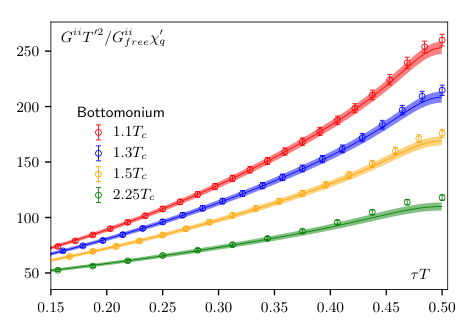
that largely removes the transport contribution mostly present in the large region. We fit this using an ansatz consisting only of the perturbative part, i.e. . The obtained values of fit parameters A and B are listed in tab. 2. As seen from fig. 2, the fit results match the lattice data well. We also computed the correlation function from the fit spectral function and show the results as bands in the bottom two plots in Fig. 2. The differences between the bands and lattice data points hint to the transport contribution.
To further investigate the small part of the spectral function, we fix the values for and and calculate the difference of the lattice data and the fit results
| (7) |
Since the midpoint contains the largest contribution from transport effects and the curvature of the correlator is negligible, section 4.1 focuses on .


| Charmonium | Bottomonium | |||
|---|---|---|---|---|
| 1.1 | 1.09(2) | 0.37(4) | 1.03(2) | 0.04(2) |
| 1.3 | 1.07(2) | 0.16(5) | 1.01(1) | -0.05(2) |
| 1.5 | 1.03(2) | 0.01(6) | 1.00(2) | -0.12(2) |
| 2.25 | 0.99(3) | -0.27(9) | 0.99(2) | -0.23(4) |
4.1 Transport contribution
Fig. 3 shows the temperature dependence of the transport contribution at the midpoint. It is clearly seen that the transport contribution for charmonium increases with temperature, while for bottomonium the results are almost constant in temperature within errors. Another observation is that for 1.5 and 2.25 the charmonium result lies above the bottomonium result. This can be used to conclude a relation between the drag coefficients of charm and bottom quarks. To reach this goal, we expand the kernel and the cut-off term from (4) at the midpoint around as
| (8) |
We now insert (4) into the correlator and make use of the above simplication. With the Einstein relation we arrive at
| (9) |
The dominant contribution comes from and higher orders can be neglected. When we insert the charmonium and bottomonium masses, we obtain
| (10) |
The ratio of the masses is roughly 3 and when comparing this to the lattice data, we can conclude that , which is only fulfilled when the charm quark drag coefficient is larger than that of the bottom quark . We have checked the relative strength of drag coefficients using a Gaussian ansatz and also holds.
4.2 Bound state region
By fitting the differences of neighboring correlators we obtain a result for the high region of our spectral function in the vector channel. As in the pseudoscalar channel, the overall normalization is close to 1 and the mass shift is small. With these slight modifications, the perturbative spectral function is well-suited to describe the bound state region. The results are shown in fig. 4. For charmonium the model spectral function describes the data well without a resoncance peak while for bottomonium including one thermally broadened peak that vanishes at 2.25 consistently describes the continuum extrapolated lattice data.


5 Conclusion
In this work, we found good agreement between our continuum extrapolated lattice correlators in the vector channel and a perturbative spectral function constructed by combining vacuum asymptotics with pNRQCD. By accounting for systematical uncertainties, we were able to present a modified version of the perturbative spectral function for the bound state regime that describes the correlator data almost perfectly. We split the analysis of the vector correlators in two seperate parts and fix the bound state region via fits to the difference of neighbouring correlators. We found that charmonium correlators in the vector channel can be well reproduced by perturbative spectral functions, where no resonance peaks for are needed at and above 1.1, while for bottomonia correlators a thermally broadened resonance peak for persists up to . From the analysis of the transport contribution we find that the charm quark drag coefficient is larger than the bottom quark drag coefficient. A further analysis of the transport peak we are currently following [9] is to investigate the transport coefficients in more detail by comparing the lattice result at the midpoint to different ansätze for the transport peak.
6 Acknowledgements
This work was supported by the Deutsche Forschungsgemeinschaft (DFG, German Research Foundation) – project number 315477589 – TRR 211, NSFC under grant numbers 11775096 and 11535012.
References
- [1] A. Rothkopf, Heavy Quarkonium in Extreme Conditions, arXiv:1912.02253
- [2] H.-T. Ding, F. Karsch, S. Mukherjee, Thermodynamics of strong-interaction matter from Lattice QCD, Int. J. Mod. Phys.E24(2015),1530007, arXiv:1504.05274
- [3] Y. Burnier, H.-T. Ding, O. Kaczmarek, A.-L. Kruse, M. Laine, H. Ohno, H. Sandmeyer, Thermal quarkonium physics in the pseudoscalar channel, JHEP 11(2017),206, arXiv:1709.07612
- [4] P. Petrecky, D. Teany, Heavy Quark Diffusion from the Lattice, Phys. Rev. D 73(2006),014508, arXiv:hep-ph/0507318
- [5] Y. Burnier, M. Laine, Eur. Phys. J., Towards flavour diffusion coefficient and electrical conductivity without ultraviolet contamination, C72(2012),1902, arXiv:1201.1994
- [6] M. Laine, A resummed perturbative estimate for the quarkonium spectral function in hot QCD, JHEP 05(2007),028, arXiv:0704.1720
- [7] H.-T. Ding, O. Kaczmarek, A.-L. Kruse, H. Ohno, H. Sandmeyer, Continuum extrapolation of quarkonium correlators at non-zero temperature, EPJ Web Conf. 175(2018),07010, arXiv:1710.08858
- [8] Y. Burnier, M. Laine, Massive vector current correlator in thermal QCD, JHEP 1211(2012),086, arXiv:1210.1064
- [9] H.-T. Ding, O. Kaczmarek, A.-L. Lorenz, H. Ohno, H. Sandmeyer, H.-T. Shu, work in progress