ٔDynamic Frame Structure for Next Generation Wireless Networks

3GPP has categorized the network services into enhanced mobile broadband (eMBB), massive machine-type communications (mMTC), and ultra-reliable and low-latency communications (URLLC) services [1]. eMBB services, like video streaming, require high data rate connections; mMTC services, like internet of things (IoT), require large number of devices to connect to the network which would only send small data payloads; and URLLC services, like tactile Internet (TI), require communications of small payloads with low-latency and very high reliability. Due to heterogeneous requirements of these services, the efficient and dynamic resource allocation in the network is the main challenge. Traditional resource block structure (RBS) definition with fixed time-frequency structure, e.g., as in LTE with 1 millisecond transmission time interval (TTI) and 15 kHz bandwidth, is not able to support the network with these three types of services [1, 2]. The eMMB services require many frequency resources to satisfy their data rate requirements whose latency is not of importance, and hence, the time duration of the allocated RBs could be high, e.g., above one millisecond. On the other hand, URLLC services have small packets for transmission and require that these packets are sent in short time intervals, e.g., 0.1 to 0.5 milliseconds, with high reliability. In 4G, The admitted end-to-end latency of 4G networks is 30$\sim$100 milliseconds and the target reliability of information transmission is 0.99 which is not sufficient for ultra reliable services such as virtual reality and autonomous deriving, which is equal to 0.99999. In 5G, the RBs with different TTIs and bandwidths can satisfy latency and reliability requirements of services. In these networks, the notion of RB is defined as a time-frequency block with different time durations and bandwidths. In other words, the total time duration and bandwidth, e.g., $T$ milliseconds time duration and $W$ Hz bandwidth, is partitioned into several RBs with different time durations, e.g., $T$, $\frac{T}{2}$, and $\frac{T}{4}$, and different bandwidths, e.g., $W$, $\frac{W}{2}$, and $\frac{W}{4}$. Different RBs with different time durations and bandwidths can be used for different services based on the service requirements.

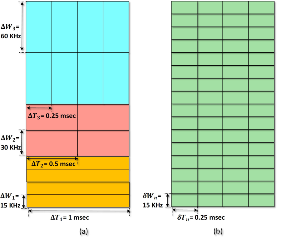
In the aforementioned structure, although the size of the RBs is different, the size of each RB is predetermined and fixed. We call this structure by static RBS (S-RBS) as the size of the RBs is predefined and cannot be changed. However, this RB structure, due to fixed TTI and bandwidth, does not have enough flexibility to satisfy different service requirements in an efficient way. Therefore, we propose a dynamic RBS (D-RBS) for 5G in which the total time duration and bandwidth is partitioned into several small RBs of equal time duration and bandwidth. Based on the service requirements, some small RBs are aggregated to form a composite RB¹¹ 1 We call the aggregated small blocks which are allocated to a user by composite resource block used by one specific service. In other words, the allocated RBs to each user can be constructed using one or more of these small RBs which could be spanned over different time and frequency bands. Dynamic here means that the size of the ultimate RBs is not predefined and could be different. The proposed structure enables dynamic allocation of RBs leading to efficient network resource utilization.

Our proposed approach can also be easily extended to network slicing where each type of user belongs to one slice. Network slicing is a kind of virtual networking architecture. Its structure allows the creation of multiple virtual networks with different rate and latency requirements atop a shared physical infrastructure.

The resource allocation problem among 5G network’s services has been addressed in several works [3, 4]. The authors in [3] study the downlink multiplexing of URLLC and eMBB services. The goal is to maximize the utility for eMBB traffic with respect to URLLC service requirement constraints. In [4], the authors study the downlink of 5G networks for URLLC services with the aim of achieving trade off between SE, latency, and reliability for each link and service flow. The dynamic scheduling for mMTC and URLLC services is studied in [5] for NR where the authors investigate the performance of feedbackless and feedback based frameworks based on reinforcement learning. They illustrate that both schemes are able to effectively deploy both URLLC and mMTC services in NR. Recently, individual service designing has attracted a lot of attentions and there are several researches on RB design in wireless networks [6, 7, 8, 9, 3]. An overview of 5G deployment challenges are provided in [6]. In [7], the authors provide a survey of key techniques to overcome the new requirements and challenges of mMTC applications. The principles of using diversity sources, design of packets, and access protocols to support URLLC are investigated in [8]. In [9], the authors provide joint power and subchannel allocation for sliced 5G network with respect to both the inter-tier and intra-tier interference constraints. In [10], the authors study orthogonal resource allocation for mMTC and eMBB. The uplink multiplexing of URLLC, eMBB, and mMTC services is studied in [11]. In [12], the authors investigate downlink transmission design for URLLC services. Joint resource allocation in uplink and downlink based on effective bandwidth and effective capacity to ensure the quality of service (QoS) for URLLC is considered in [13, 14]. Joint uplink and downlink bandwidth optimization with respect to delay constraints to guarantee both packet loss constraint and end-to-end delay requirement is considered in [14]. In [15], the authors propose a packet delivery mechanism for URLLC. The goal is to reduce the bandwidth required to guaranteeing queuing delay based on statistical multiplexing queuing model. The network slicing based on orthogonal and non-orthogonal radio resource allocation for the three types of services of 5G is considered in [16]. In [17], the authors optimize power and bandwidth allocation across radio access network slices and users which have heterogeneous QoS requirements. The goal is to maximize both throughput and energy efficiency in the sliced radio access network. In [18, 5], the authors investigate the dynamic downlink resource allocation for eMBB and URLLC services on the same time/frequency resources. The impact of 5G frame structure on URLLC performance is investigated in [19]. The performance of flexible TTI to adopt traffic load is investigated in [20, 21]. A 5G frame structure designing is considered in [4] to support user’s service requirements. In all the previous works, the authors have considered a static structure for RBs that does not have enough flexibility to respond to different service requirements. Indeed, they do not consider both outage and bit error rate constraints that are critical for new emerging services in 5G. In fact, since the traditional framing, resource allocation, and user association schemes are not flexible enough and do not consider various service types requirements in their optimization problems, they are not appropriate for 5G services.

In this paper, we propose and design a dynamic framing scheme for supporting different types of services in the network, i.e., D-RBS, and investigate its performance. In contrast to the S-RBS scheme, in the proposed scheme, composite RBs are flexible in that the constructing small blocks could be of different time durations in different frequency bands, and the number of allocated small blocks us determined by the adopted resource allocation algorithm.

In D-RBS, it is assumed that each cell partitions the total time duration and bandwidth in its own way which is determined by the resource allocation framework. The resulting partitioned resource blocks would be different for different cells. More precisely, we devise and develop a new resource management framework for wireless networks with different types of services each with different requirements where the time-frequency resource of the network is partitioned into several composite RBs each having different number of small RBs To this end, we formulate our proposed scheme as an optimization problem whose outcome is joint dynamic frame structure design, resource allocation, and user association (matching of users to RBs). Our aim is to maximize the network throughput under transmit power constraints and QoS requirements of eMBB, mMTC, and URLLC services. Our contributions are as follows:

• •

  We design a new dynamic frame resource management scheme for next generations of wireless networks where different services have different QoS requirements which in turn requires different time-bandwidth resources. In the proposed scheme, the resource management algorithm provides joint RB partitioning, resource allocation, and user association.

• •

  We formulate our proposed resource management scheme as optimization problems which are mixed integer nonlinear nonconvex optimization problems in general. The alternate search method (ASM) is used to decompose the main optimization problem into to optimization sub-problem. In the first optimization sub-problem, given RB assignment, we optimize the power allocation. In the second optimization sub-problem, given the power allocation results of the first sub-problem, we optimize the RB association. To solve the resulting non-convex sub-problems at each level, we exploit the successive convex approximation (SCA) method to write the main non-convex problem into a series of convex problems which could be solved using standard tools like CVX.

• •

  We study the convergence of our proposed scheme and show that the algorithms converge to a sub-optimal solution. We further investigate our proposed scheme from the computational complexity prespective.

• •

  We provide a global optimization solution by means of the monotonic optimization method.

• •

  We study the performance of the proposed scheme using simulations for different network parameters. We show the superiority of our scheme and show that the performance of D-RBS is better than that of the S-RBS scheme due to its dynamic nature which is suitable for highly dynamic environment of wireless networks.

The remainder of this paper is organized as follows. System model and descriptions regarding 5G services and requirements are presented in Section II. Problem formulation and solution algorithms are provided in Section III. In Section IV, we provide global optimization solution by monotonic optimization method. In Section V, we provide the convergence proof and the computational complexity of our scheme. Simulation results are provided in Section VI. And finally, Section VII concludes this work.

We consider a multi-cell downlink of an OFDMA network. There is one BS at each cell. The BS set is denoted by $\mathcal{B}=\{1,2,\dots,B\}$ with $|\mathcal{B}|=B$ where $|.|$ denotes the number of elements in a set. There are three types of users which request different types of services. In BS $b$, the sets of users which request eMBB, mMTC, and URLLC services are demoted by $\mathcal{K}^{\text{e}}_{b}=\{1,2,\dots,K^{\text{e}}_{b}\}$, $\mathcal{K}^{\text{m}}_{b}=\{1,2,\dots,K^{\text{m}}_{b}\}$ and $\mathcal{K}^{\text{u}}_{b}=\{1,2,\dots,K^{\text{u}}_{b}\}$, respectively, with $|\mathcal{K}^{\text{e}}_{b}|=K^{\text{e}}_{b}$, $|\mathcal{K}^{\text{m}}_{b}|=K^{\text{m}}_{b}$ and $|\mathcal{K}^{\text{u}}_{b}|=K^{\text{u}}_{b}$. The set of total user in BS $b$ is denoted by $\mathcal{K}_{b}=\mathcal{K}^{\text{e}}_{b}\cup\mathcal{K}^{\text{m}}_{b}\cup\mathcal{K}^{\text{u}}_{b}$ and $K_{b}=|\mathcal{K}_{b}|$ denotes the total number of users in BS $b$. The BSs and users are equipped with one antenna. A time-frequency resource of $T$ seconds and $W$ Hz is used by each cell. In the proposed frame structure, we assume that the time-frequency resource is divided into several small RBs with the time duration $\chi$ and frequency size $\vartheta$. All the small RBs could be shown by a matrix $[A]_{F\times N}$ with $N=\frac{T}{\chi}$ and $F=\frac{W}{\vartheta}$. In contrast to the S-RBS scheme, in which the size of RBs are constant (Fig. 1), in the proposed scheme, at each cell, users are flexibly multiplexed over these small RBs. To each user several small RBs may be assigned which could be in different times and frequency bands and be noncontiguous in time and frequency. This RB structure is shown in Fig. 1.

With carrier and slot aggregation capability, already in use [22], we can aggregate radio carriers (in the same band or across disparate bands) and slots of different small blocks to construct composite RBs to meet the requirements of users. Therefore, for user $k$ in cell $b$, the assigned composite RB is constructed by aggregation of one or more small blocks of time duration $\chi$ and frequency size $\vartheta$. Then, the users are multiplexed in an orthogonal fashion to the composite RBs.

The eMBB service requires high bandwidth and the reliability, given by packet error rate (PER), about $10^{-3}$ [1]. The instantaneous transmission rate between the $b^{\text{th}}$ BS and the $k^{\text{th}}$ user on RB $(f,n)$ is defined as

where $I^{fn}_{bk}(\textbf{p},\textbf{s},\textbf{g})=\sum_{i\in\mathcal{B}\setminus\{b\}}\sum_{j\in\mathcal{K}_{i}\setminus\{k\}}s^{fn}_{ij}p^{fn}_{ij}g^{fn}_{ik}$ is the interference to user $k$ in cell $b$ on RB $(f,n)$, $p^{fn}_{bk}$ and $g^{fn}_{bk}$ are the transmit power and channel power gain of the $b^{\text{th}}$ BS to the $k^{\text{th}}$ user on RB $(f,n)$, respectively, while $N_{0}$ is the single-sided noise power-spectral-density (PSD). $\textbf{g}=[g^{11}_{11},\dots,g^{fn}_{bk},\dots,g^{FN}_{BK}]^{T}$, $\textbf{p}=\{p^{11}_{11},\dots,p^{fn}_{bk},\dots,p^{FN}_{BK}\}$, and $\textbf{s}=\{s^{11}_{11},\dots,s^{fn}_{bk},\dots,s^{FN}_{BK}\}$ denote the channel gain, the power allocation and small RBs assignment vectors.

The binary-valued RB-association factor $s^{fn}_{bk}$ represents both RB and BS assignment indicator for user $k$ of BS $b$ on RB $(f,n)$, i.e., $s^{fn}_{bk}=1$ when BS $b$ allocates RB $(f,n)$ to user $k$, and $s^{fn}_{bk}=0$, otherwise. For user $k$ which requests eMBB service, the following constraint should be satisfied to ensure that the data rate of user $k$ is equal or above the required minimum data rate:

where $R^{\text{min,e}}_{bk}$ denotes the required data rate of eMBB user $k$ at BS $b$.

The URLLC service requires low-latency and very high reliability transmission with packet loss probability lower than $10^{-7}$ [1]. The achievable rate of user $k$ in RB $(f,n)$ with finite block length can be accurately approximated as follows [23, 24]:

where $\gamma^{fn}_{bk}(\textbf{p},\textbf{s},\textbf{g})=\frac{p^{fn}_{bk}g^{fn}_{bk}}{\sum_{i\in\mathcal{B}\setminus\{b\}}\sum_{j\in\mathcal{K}_{i}\setminus\{k\}}s^{fn}_{ij}p^{fn}_{ij}g^{fn}_{ik}+\vartheta N_{0}}$, $f^{-1}_{Q}(.)$ is the inverse of Gaussian-Q function, $\nu^{fn}_{bk}=1-\frac{1}{(1+\gamma^{fn}_{bk})^{2}}$ and $\varepsilon^{fn}_{bk}$ denotes the decoding error probability. The number of symbols in the block is $\psi=\chi\vartheta$. When transmitting $\kappa$ bits from BS $b$ to user $k$ in the short blocklength regime, by setting $\chi R^{\text{URLLC},fn}_{bk}=\kappa$, the decoding error probability can be obtained from (3) as follows:

where $\mathbb{E}(x)$ denotes the expected value of $x$. Unfortunately, a closed-form expression for Q-function does not exist. Hence, we utilize an approximation of $f_{Q}\left(\frac{\log_{2}\left(1+\gamma^{fn}_{bk}(\textbf{p},\textbf{s},\textbf{g})\right)-\hat{\varphi}}{\sqrt{\nu^{fn}_{bk}(\gamma^{fn}_{bk}(\textbf{p},\textbf{s},\textbf{g}))(\log_{2}e)^{2}/\psi}}\right)\approx\Gamma(\gamma^{fn}_{bk}(\textbf{p},\textbf{s},\textbf{g}))$ to approximate the decoding error probability [25], where $\hat{\varphi}=\kappa/\psi$ is the number of bits in each symbol,

where $\varpi=\frac{1}{2\pi\sqrt{2^{2\hat{\varphi}}-1}}$, $\theta=2^{\hat{\varphi}}-1$, $\eta_{1}=\theta-\frac{1}{2\varpi\sqrt{\psi}}$, and $\eta_{2}=\theta+\frac{1}{2\varpi\sqrt{\psi}}$.

The following constraint should be satisfied to ensure that the packet loss probability of user $k$ in RB $(f,n)$ is equal or below the threshold value $\varepsilon^{\text{max},fn}_{bk}$:

Due to the delay limitation of URLLC users, the following constraint is used:

which means that each URLLC user is assigned to only one RBs column (i.e., one column of small RBs over the entire spectrum and one TTI). More specifically, (7) ensures when any RBs in one RB column is assigned to one URLLC user, that URLLC user would not be assigned any RBs in other RB columns.

The mMTC users require fixed, typically low, transmission rate and PER on the order of $10^{-1}$ [1]. To guarantee these requirements, the following constraints should be applied:

and the following constraint should be satisfied to ensure that the packet loss probability of user $k$ in RB $(f,n)$ is equal or below the threshold values $\tilde{\varepsilon}^{\text{max},fn}_{bk}$:

Given s, the following power allocation optimization sub-problem to maximize the total rate should be solved:

Problem $\mathcal{P}^{\text{D-RBS}}_{\text{PA}}$

Optimization problem (11) is non-convex, due to the interference term in the objective function and constraints (2), (6), (8), and (9). We convert (11) into the GP optimization problem. In this regards, we rewrite the objective of (11) as:

where $\Gamma^{fn}_{bk}(\textbf{p}(\varrho_{1}),\textbf{s}(\varrho),\textbf{g})=\frac{\vartheta N_{0}+I^{fn}_{bk}(\textbf{p}(\varrho_{1}),\textbf{s}(\varrho),\textbf{g})+p^{fn}_{bk}(\varrho_{1})g^{fn}_{bk}}{\vartheta N_{0}+I^{fn}_{bk}(\textbf{p}(\varrho_{1}),\textbf{s}(\varrho),\textbf{g})}$. Arithmetic-geometric mean approximation (AGMA) method is exploited for posynomial form approximation [27]. Therefore, $[\Gamma^{fn}_{bk}(\textbf{p}(\varrho_{1}),\textbf{s}(\varrho),\textbf{g})]^{-1}$ can be approximated as [27]

where

Furthermore, we provide convex approximations for non-convex constraints (6) and (9). To this end, we use the first order Taylor series approximation of $\gamma^{fn}_{bk}(\textbf{p}(\varrho_{1}),\textbf{s}(\varrho),\textbf{g})$ around $\textbf{p}(\varrho_{1}-1)$, i.e., $\tilde{\gamma}^{fn}_{bk}(\textbf{p}(\varrho_{1}))$, as follows:

where the gradient $\nabla\gamma^{fn}_{bk}(\textbf{p}(\varrho_{1}),\textbf{s}(\varrho),\textbf{g})$ with respect to $\mathbf{p}$ is given by

where

Thus, the constraints (6) and (9) can be rewritten as follows:

Consequently, (11) can be transformed into standard GP problem as follows:

Problem $\check{\mathcal{P}}^{\text{D-RBS}}_{\text{PA}}$

With the value of $\textbf{p}(\varrho)$ from power allocation problem, the following RB assignment optimization problem is solved:

Problem $\mathcal{P}^{\text{D-RBS}}_{\text{RBA}}$

Due to objective function and constraints (22a), (2), and (8), the optimization problem is non-convex. We first relax discrete variable $s^{fn}_{bk}(\varrho_{2})$ into continuous one as $s^{fn}_{bk}(\varrho_{2})\in[0,1]$. By exploiting AGMA, we transform problem (22) to a standard for of GP. Note that in the same way in (16), we can use the first order Taylor series approximation of $\gamma^{fn}_{bk}(\textbf{p}(\varrho),\textbf{s}(\varrho_{2}),\textbf{g})$ around $s^{fn}_{bk}(\varrho_{2}-1)$. Defining $\alpha^{n}_{bk}(\varrho_{2})=\sum_{f\in\mathcal{F}}s^{fn}_{bk}(\varrho_{2})$ and $\beta_{bk}(\varrho_{2})=\sum_{f\in\mathcal{F}}\sum_{n\in\mathcal{N}}s^{fn}_{bk}(\varrho_{2})$, one can approximate (7) by the following constraints:

where $\omega^{n}_{bk}(\varrho_{2})$ is an an auxiliary variable,

Based on (23a)-(23d), (7) is replaced by monomial equalities and posynomial inequalities. Next, we convert the objective function and write it into monomial form. By defining the auxiliary variables $\zeta_{1}$ and $\zeta_{2}$, (22) is written into the following standard for of GP:

Problem $\check{\mathcal{P}}^{\text{D-RBS}}_{\text{RBA}}$

References

- [1] 3GPP, Study on Scenarios and Requirements for Next Generation Access Technologies, Technical Specification Group Radio Access Network, Technical Report 38.913, Release 14, October 2016.
- [2] ——, LTE; Evolved Universal Terrestrial Radio Access (E-UTRA); Physical channels and modulation, Technical Specification Group Radio Access Network, Technical Report 36.211, Release 10, January 2011.
- [3] A. Anand, G. de Veciana, and S. Shakkottai, “Joint scheduling of URLLC and eMBB traffic in 5G wireless networks,” arXiv preprint arXiv:1712.05344, 2017.
- [4] K. I. Pedersen, G. Berardinelli, F. Frederiksen, P. Mogensen, and A. Szufarska, “A flexible 5G frame structure design for frequency-division duplex cases,” IEEE Communications Magazine, vol. 54, no. 3, pp. 53–59, March 2016.
- [5] S.-Y. Lien, S.-C. Hung, D.-J. Deng, and Y. J. Wang, “Efficient ultra-reliable and low latency communications and massive machine-type communications in 5G new radio,” in Proceeding of IEEE Global Communications Conference (GLOBECOM), pp.1–7, December 2017, Singapore, Singapore.
- [6] M. Shafi, A. F. Molisch, P. J. Smith, T. Haustein, P. Zhu, P. De Silva, F. Tufvesson, A. Benjebbour, and G. Wunder, “5G: A tutorial overview of standards, trials, challenges, deployment, and practice,” IEEE Journal on Selected Areas in Communications, vol. 35, no. 6, pp. 1201–1221, April 2017.
- [7] Z. Dawy, W. Saad, A. Ghosh, J. G. Andrews, and E. Yaacoub, “Toward massive machine type cellular communications,” IEEE Wireless Communications, vol. 24, no. 1, pp. 120–128, November 2017.
- [8] P. Popovski, J. J. Nielsen, C. Stefanovic, E. de Carvalho, E. Strom, K. F. Trillingsgaard, A. S. Bana, D. M. Kim, R. Kotaba, J. Park et al., “Wireless access for ultra-reliable low-latency communication: Principles and building blocks,” IEEE Network, vol. 32, no. 2, pp. 16–23, April 2018.
- [9] H. Zhang, N. Liu, X. Chu, K. Long, A.-H. Aghvami, and V. C. Leung, “Network slicing based 5G and future mobile networks: mobility, resource management, and challenges,” IEEE Communications Magazine, vol. 55, no. 8, pp. 138–145, August 2017.
- [10] N. H. Mahmood, M. Lauridsen, G. Berardinelli, D. Catania, and P. Mogensen, “Radio resource management techniques for eMBB and mMTC services in 5G dense small cell scenarios,” in Proceedings of Vehicular Technology Conference (VTC-Fall), pp.1–5, September 2016, Montreal, QC, Canada.
- [11] L. Tian, C. Yan, W. Li, Z. Yuan, W. Cao, and Y. Yuan, “On uplink non-orthogonal multiple access for 5G: opportunities and challenges,” China Communications, vol. 14, no. 12, pp. 142–152, December 2017.
- [12] C. She, C. Yang, and T. Q. Quek, “Cross-layer optimization for ultra-reliable and low-latency radio access networks,” IEEE Transactions on Wireless Communications, vol. 17, no. 1, pp. 127–141, October 2018.
- [13] A. Aijaz, “Towards 5G-enabled tactile internet: Radio resource allocation for haptic communications,” in Proceedings of Wireless Communications and Networking Conference (WCNC), pp.1–6, April 2016, Doha, Qatar.
- [14] C. She, C. Yang, and T. Q. Quek, “Radio resource management for ultra-reliable and low-latency communications,” IEEE Communications Magazine, vol. 55, no. 6, pp. 72–78, June 2017.
- [15] ——, “Joint uplink and downlink resource configuration for ultra-reliable and low-latency communications,” arXiv preprint arXiv:1801.00988, 2018.
- [16] P. Popovski, K. F. Trillingsgaard, O. Simeone, and G. Durisi, “5G wireless network slicing for eMBB, URLLC, and mMTC: A communication-theoretic view,” arXiv preprint arXiv:1804.05057, 2018.
- [17] B. Matthiesen, O. Aydin, and E. A. Jorswieck, “Throughput and energy-efficient network slicing,” in WSA 2018; 22nd International ITG Workshop on Smart Antennas. VDE, 2018, pp. 1–6.
- [18] Z. Wu, F. Zhao, and X. Liu, “Signal space diversity aided dynamic multiplexing for eMBB and URLLC traffics,” in Proceedings of International Conference on Computer and Communications (ICCC), pp.1396–1400, March 2017, Chengdu, China.
- [19] M. Iwabuchi, A. Benjebbour, Y. Kishiyama, G. Ren, C. Tang, T. Tian, L. Gu, T. Takada, and T. Kashima, “5G field experimental trials on uRLLC using new frame structure,” in Globecom Workshops (GC Wkshps), 2017 IEEE. IEEE, 2017, pp. 1–6.
- [20] Q. Liao, P. Baracca, D. Lopez-Perez, and L. G. Giordano, “Resource scheduling for mixed traffic types with scalable TTI in dynamic TDD systems,” in Proceeding of Globecom Workshops, pp.1–7, December 2016, Washington, DC, USA.
- [21] E. Fountoulakis, N. Pappas, Q. Liao, V. Suryaprakash, and D. Yuan, “An examination of the benefits of scalable TTI for heterogeneous traffic management in 5G networks,” in Proceeding of International Symposium on Modeling and Optimization in Mobile, Ad Hoc, and Wireless Networks (WiOpt), pp.1–6, May 2017, Paris, France.
- [22] G. T. . 912, “5G; study on new radio access technology,” TECHNICAL REPORT, V14.1.0 (2017-10).
- [23] G. Durisi, T. Koch, and P. Popovski, “Toward massive, ultrareliable, and low-latency wireless communication with short packets,” Proceedings of the IEEE, vol. 104, no. 9, pp. 1711–1726, 2016.
- [24] W. Yang, G. Durisi, T. Koch, and Y. Polyanskiy, “Quasi-static multiple-antenna fading channels at finite blocklength,” IEEE Transactions on Information Theory, vol. 60, no. 7, pp. 4232–4265, 2014.
- [25] B. Makki, T. Svensson, and M. Zorzi, “Finite block-length analysis of the incremental redundancy HARQ,” IEEE Wireless Communications Letters, vol. 3, no. 5, pp. 529–532, 2014.
- [26] S. Boyd and L. Vandenberghe, Convex optimization. Cambridge university press, 2004.
- [27] P. Shen and K. Zhang, “Global optimization of signomial geometric programming using linear relaxation,” Applied Mathematics and Computation, vol. 150, no. 1, pp. 99–114, 2004.
- [28] M. Chiang, C. W. Tan, D. P. Palomar, D. O’neill, and D. Julian, “Power control by geometric programming,” IEEE Transactions on Wireless Communications, vol. 6, no. 7, pp. 2640–2651, July 2007.
- [29] B. R. Marks and G. P. Wright, “A general inner approximation algorithm for nonconvex mathematical programs,” Operations research, vol. 26, no. 4, pp. 681–683, 1978.
- [30] Y. J. A. Zhang, L. Qian, J. Huang et al., “Monotonic optimization in communication and networking systems,” Foundations and Trends® in Networking, vol. 7, no. 1, pp. 1–75, 2013.
- [31] M. Moltafet, P. Azmi, N. Mokari, M. R. Javan, and A. Mokdad, “Optimal and fair energy efficient resource allocation for energy harvesting-enabled-pd-noma-based hetnets,” IEEE Transactions on Wireless Communications, vol. 17, no. 3, pp. 2054–2067, 2018.