跳到论文正文
W Papers独立论文阅读器 arXiv:2002.00288 论文正文 计算阅读时间 · 0%
引用这篇论文根据当前论文元数据生成,正式投稿前建议核对。


License: CC BY 4.0
arXiv:2002.00288v1 [stat.ML] 01 Feb 2020
 

The Sylvester Graphical Lasso (SyGlasso)


Yu Wang          Byoungwook Jang          Alfred Hero

University of Michigan wayneyw@umich.edu          University of Michigan bwjang@umich.edu          University of Michigan hero@umich.edu

Abstract

This paper introduces the Sylvester graphical lasso (SyGlasso) that captures multiway dependencies present in tensor-valued data. The model is based on the Sylvester equation that defines a generative model. The proposed model complements the tensor graphical lasso (Greenewald et al., 2019) that imposes a Kronecker sum model for the inverse covariance matrix by providing an alternative Kronecker sum model that is generative and interpretable. A nodewise regression approach is adopted for estimating the conditional independence relationships among variables. The statistical convergence of the method is established, and empirical studies are provided to demonstrate the recovery of meaningful conditional dependency graphs. We apply the SyGlasso to an electroencephalography (EEG) study to compare the brain connectivity of alcoholic and nonalcoholic subjects. We demonstrate that our model can simultaneously estimate both the brain connectivity and its temporal dependencies.

1 Introduction

Estimating conditional independence patterns of multivariate data has long been a topic of interest for statisticians. In the past decade, researchers have focused on imposing sparsity on the precision matrix (inverse covariance matrix) to develop efficient estimators in the high-dimensional statistics regime where n≪pn\ll p. The success of the ℓ1\ell_{1}-penalized method for estimating multivariate dependencies was demonstrated in Meinshausen and Bühlmann, 2006 and Friedman et al., 2008 for the multivariate setting. This has naturally led researchers to generalize these methods to multiway tensor-valued data. Such generalizations are of benefit for many applications, including the estimation of brain connectivity in neuroscience, reconstruction of molecular networks, and detecting anomalies in social networks over time.

The first generalizations of multivariate analysis to the tensor-variate settings were presented by Dawid, 1981, where the matrix-variate (a.k.a. two-dimensional tensor) distribution was first introduced to model the dependency structures among both rows and columns. Dawid, 1981 extended the multivariate setting by rewriting the tensor-variate data as a vectorized (vec) representation of the tensor samples 𝓧∈ℝm1×⋯×mk\bm{\mathcal{X}}\in\mathbb{R}^{m_{1}\times\cdots\times m_{k}} and analyzing the overall precision matrix 𝛀=𝔼⁡(vec​(𝓧)​vec​(𝓧)T)∈ℝm×m\mathbf{\Omega}=\mathbb{E}\big(\text{vec}(\bm{\mathcal{X}})\text{vec}(\bm{\mathcal{X}})^{T}\big)\in\mathbb{R}^{m\times m}, where m=∏k=1Kmkm=\prod_{k=1}^{K}m_{k}. Even for a two-dimensional tensor 𝓧∈ℝm1×m2\bm{\mathcal{X}}\in\mathbb{R}^{m_{1}\times m_{2}}, the computation complexity and sample complexity is high since the number of parameters in the precision matrix grows quadratically as m2m^{2}. Therefore, in the regime of tensor-variate data, unstructured precision matrix estimation has posed challenges due to the large number of samples needed for accurate structure recovery.

To address the sample complexity challenges, sparsity can be imposed on the precision matrix 𝛀\mathbf{\Omega} by using a sparse Kronecker product (KP) or Kronecker sum (KS) decompositions of 𝛀\mathbf{\Omega}. The earliest and most popular form of sparse structured precision matrix estimation represents 𝛀\mathbf{\Omega} as the Kronecker product of smaller precision matrices. Tsiligkaridis et al., 2013 and Zhou, 2014 proposed to model the precision matrix as a sparse Kronecker product of the covariance matrices along each mode of the tensor in the form 𝛀=𝚿1⊗⋯⊗𝚿K\bm{\Omega}=\bm{\Psi}_{1}\otimes\cdots\otimes\bm{\Psi}_{K}. The KP structure on the precision matrix has the nice property that the corresponding covariance matrix is also a KP. Zhou, 2014 provides a theoretical framework for estimating the 𝛀\mathbf{\Omega} under KP structure and showed that the precision matrices can be estimated from a single instance under the matrix-variate normal distribution. Lyu et al., 2019 extended the KP structured model to tensor-valued data, and provided new theoretical insights into the KP model. An alternative, called the Bigraphical Lasso, was proposed by Kalaitzis et al., 2013 to model conditional dependency structures of precision matrices by using a Kronecker sum representation 𝛀=𝚿1⊕𝚿2=(𝚿1⊗𝐈)+(𝐈⊗𝚿2)\bm{\Omega}=\bm{\Psi}_{1}\oplus\bm{\Psi}_{2}=(\bm{\Psi}_{1}\otimes\mathbf{I})+(\mathbf{I}\otimes\bm{\Psi}_{2}). On the other hand, Rudelson and Zhou, 2017 and Park et al., 2017 studied the KS structure on the covariance matrix 𝚺=𝐀⊕𝐁\bm{\Sigma}=\mathbf{A}\oplus\mathbf{B} which corresponds to errors-in-variables models. More recently, Greenewald et al., 2019 proposed a model that generalized the KS structure to model tensor-valued data, called the TeraLasso. As shown in their paper, compared to the KP structure, KS structure on the precision matrix leads to a non-separable covariance matrix that provides a richer model than the KP structure.

KP vs KS: The KP model admits a simple stochastic representation as 𝐗=𝐂−1​𝐙𝐃−1\mathbf{X}=\mathbf{C}^{-1}\mathbf{Z}\mathbf{D}^{-1}, where 𝐀=𝐂𝐂T,𝐁=𝐃𝐃T\mathbf{A}=\mathbf{C}\mathbf{C}^{T},\mathbf{B}=\mathbf{D}\mathbf{D}^{T}, and 𝐙\mathbf{Z} is white Gaussian. It can be shown using properties of KP that X∼𝒩⁡(0,(𝐀⊗𝐁)−1)X\sim\mathcal{N}(0,(\mathbf{A}\otimes\mathbf{B})^{-1}). Unlike the KP model, the KS model does not have a simple stochastic representation. From another perspective, the Kronecker structures can be characterized by the product graphs of the individual components. Kalaitzis et al., 2013 first motivated the KS structure on the precision matrix by relating (𝚿1⊕⋯⊕𝚿K)(\mathbf{\Psi}_{1}\oplus\cdots\oplus\mathbf{\Psi}_{K}) to the associated Cartesian product graph. Thus, the overall structure of 𝛀\mathbf{\Omega} naturally leads to an interpretable model that brings the individual components together. The KP, however, corresponds to the direct tensor product of the individual graphs and leads to a denser dependency structure in the precision matrix Greenewald et al., 2019.

The Sylvester Graphical Lasso (SyGlasso): We propose a Sylvester-structured graphical model to estimate precision matrices associated with tensor data. Similar to the KP- and KS-structured graphical models, we simultaneously learn KK graphs along each mode of the tensor data. However, instead of a KS or KP model for the precision matrix, the Sylvester structured graphical model uses a KS model for the square root factor of the precision matrix. The model is estimated by joint sparse regression models that impose sparsity on the individual components 𝚿k\bm{\Psi}_{k} for k=1,…,Kk=1,\dots,K. The Sylvester model reduces to a squared KS representation for the precision matrix 𝛀=(𝚿1⊕⋯⊕𝚿K)2\mathbf{\Omega}=(\mathbf{\Psi}_{1}\oplus\cdots\oplus\mathbf{\Psi}_{K})^{2}, which is motivated by a stochastic representation of multivariate data with such a precision matrix. SyGlasso is the first KS-based graphical lasso model that admits a stochastic representation (i.e., Sylvester). Thus, our proposed SyGlasso puts the KS representations on similar ground as the KP representations in terms of interpretablility.

Notations

We adopt the notations used by Kolda and Bader, 2009. A KK-th order tensor is denoted by boldface Euler script letters, e.g, 𝓧∈ℝm1×⋯×mK\bm{\mathcal{X}}\in\mathbb{R}^{m_{1}\times\dots\times m_{K}}. 𝓧\bm{\mathcal{X}} reduces to a vector for K=1K=1 and to a matrix for K=2K=2. The (i1,…,iK)(i_{1},\dots,i_{K})-th element of 𝓧\bm{\mathcal{X}} is denoted by 𝓧i1,…,iK\bm{\mathcal{X}}_{i_{1},\dots,i_{K}}, and we define the vectorization of 𝓧\bm{\mathcal{X}} to be vec⁡(𝓧):=(𝓧1,1,…,1,𝓧2,1,…,1,…,𝓧m1,1,…,1,𝓧1,2,…,1CLOSE,\vecto(\bm{\mathcal{X}}):=(\bm{\mathcal{X}}_{1,1,\dots,1},\bm{\mathcal{X}}_{2,1,\dots,1},\dots,\bm{\mathcal{X}}_{m_{1},1,\dots,1},\bm{\mathcal{X}}_{1,2,\dots,1}, OPEN…,𝓧m1,m2,…,mk)T∈ℝm\dots,\bm{\mathcal{X}}_{m_{1},m_{2},\dots,m_{k}})^{T}\in\mathbb{R}^{m} with m=∏k=1Kmkm=\prod_{k=1}^{K}m_{k}.

There are several tensor algebra concepts that we recall. A fiber is the higher order analogue of the row and column of matrices. It is obtained by fixing all but one of the indices of the tensor, e.g., the mode-kk fiber of 𝓧\bm{\mathcal{X}} is 𝓧i1,…,ik−1,:,ik+1,…,iK\bm{\mathcal{X}}_{i_{1},\dots,i_{k-1},:,i_{k+1},\dots,i_{K}}. Matricization, also known as unfolding, is the process of transforming a tensor into a matrix. The mode-kk matricization of a tensor 𝓧\bm{\mathcal{X}}, denoted by 𝓧(k)\bm{\mathcal{X}}_{(k)}, arranges the mode-kk fibers to be the columns of the resulting matrix. It is possible to multiply a tensor by a matrix – the kk-mode product of a tensor 𝓧∈ℝm1×⋯×mK\bm{\mathcal{X}}\in\mathbb{R}^{m_{1}\times\dots\times m_{K}} and a matrix 𝐀∈ℝJ×mk\mathbf{A}\in\mathbb{R}^{J\times m_{k}}, denoted as 𝓧×k𝐀\bm{\mathcal{X}}\times_{k}\mathbf{A}, is of size m1×⋯×mk−1×J×mk+1×…​mkm_{1}\times\dots\times m_{k-1}\times J\times m_{k+1}\times\dots m_{k}. Its entry is defined as (𝓧×k𝐀)i1,…,ik−1,j,ik+1,…,iK:=∑ik=1mk𝓧i1,…,iK​Aj,ik(\bm{\mathcal{X}}\times_{k}\mathbf{A})_{i_{1},\dots,i_{k-1},j,i_{k+1},\dots,i_{K}}:=\sum_{i_{k}=1}^{m_{k}}\bm{\mathcal{X}}_{i_{1},\dots,i_{K}}A_{j,i_{k}}. In addition, for a list of matrices {𝐀1,…,𝐀K}\{\mathbf{A}_{1},\dots,\mathbf{A}_{K}\} with 𝐀k∈ℝmk×mk\mathbf{A}_{k}\in\mathbb{R}^{m_{k}\times m_{k}}, k=1,…,Kk=1,\dots,K, we define 𝓧×{𝐀1,…,𝐀K}:=𝓧×1𝐀1×2⋯×K𝐀K\bm{\mathcal{X}}\times\{\mathbf{A}_{1},\dots,\mathbf{A}_{K}\}:=\bm{\mathcal{X}}\times_{1}\mathbf{A}_{1}\times_{2}\dots\times_{K}\mathbf{A}_{K}. Lastly, we define the KK-way Kronecker product as ⨂k=1K𝚿k=𝚿1⊗⋯⊗𝚿K\bigotimes_{k=1}^{K}\bm{\Psi}_{k}=\bm{\Psi}_{1}\otimes\cdots\otimes\bm{\Psi}_{K}, and the equivalent notation for the Kronecker sum as ⨁k=1K𝚿k=𝚿1⊕⋯⊕𝚿K=∑k=1K𝐈[d1:k−1]⊗𝚿k⊗𝐈[dk+1:K]\bigoplus_{k=1}^{K}\bm{\Psi}_{k}=\bm{\Psi}_{1}\oplus\dots\oplus\bm{\Psi}_{K}=\sum_{k=1}^{K}\mathbf{I}_{[d_{1:k-1}]}\otimes\bm{\Psi}_{k}\otimes\mathbf{I}_{[d_{k+1:K}]}, where 𝐈[dk:ℓ]=𝐈dk⊗⋯⊗𝐈dℓ\mathbf{I}_{[d_{k:\ell}]}=\mathbf{I}_{d_{k}}\otimes\dots\otimes\mathbf{I}_{d_{\ell}}.

2 Sylvester Graphical Lasso

Let a random tensor 𝓧∈ℝm1×⋯×mK\bm{\mathcal{X}}\in\mathbb{R}^{m_{1}\times\dots\times m_{K}} be generated by the following representation:

𝓧×1𝚿1+⋯+𝓧×K𝚿K=𝓣,\bm{\mathcal{X}}\times_{1}\mathbf{\Psi}_{1}+\cdots+\bm{\mathcal{X}}\times_{K}\mathbf{\Psi}_{K}=\bm{\mathcal{T}}, (1)

where 𝚿k∈ℝmk×mk,k=1,…,K\mathbf{\Psi}_{k}\in\mathbb{R}^{m_{k}\times m_{k}},k=1,\dots,K are sparse symmetric positive definite matrices and 𝓣\bm{\mathcal{T}} is a random tensor of the same order as 𝓧\bm{\mathcal{X}}. Equation (1) is known as the Sylvester tensor equation. The equation often arises in finite difference discretization of linear partial equations in high dimension (Bai et al., 2003) and discretization of separable PDEs (Kressner and Tobler, 2010; Grasedyck, 2004). When K=2K=2 it reduces to the Sylvester matrix equation 𝚿𝟏​𝐗+𝐗​𝚿𝟐T=𝐓\mathbf{\Psi_{1}}\mathbf{X}+\mathbf{X}\mathbf{\Psi_{2}}^{T}=\mathbf{T} which has wide application in control theory, signal processing and system identification (see, for example Datta and Zou, 2017 and references therein).

It is not difficult to verify that the Sylvester representation (1) is equivalent to the following system of linear equations:

(⨁k=1K𝚿k)​vec⁡(𝓧)=vec⁡(𝓣),\left(\bigoplus_{k=1}^{K}\bm{\Psi}_{k}\right)\vecto(\bm{\mathcal{X}})=\vecto(\bm{\mathcal{T}}), (2)

If 𝓣\bm{\mathcal{T}} is a random tensor such that vec⁡(𝓣)\vecto(\bm{\mathcal{T}}) has zero mean and identity covariance, it follows from (2) that any 𝓧\bm{\mathcal{X}} generated from the stochastic relation (1) satisfies 𝔼​vec⁡(𝓧)=𝟎\mathbb{E}\vecto(\bm{\mathcal{X}})=\mathbf{0} and 𝚺=𝛀−1:=𝔼​vec⁡(𝓧)​vec​(𝓧)T=(⨁k=1K𝚿k)−2\mathbf{\Sigma}=\mathbf{\Omega}^{-1}:=\mathbb{E}\vecto(\bm{\mathcal{X}})\vecto(\bm{\mathcal{X}})^{T}=\left(\bigoplus_{k=1}^{K}\mathbf{\Psi}_{k}\right)^{-2}. In particular, when vec⁡(𝓣)∼𝒩⁡(𝟎,𝐈m)\vecto(\bm{\mathcal{T}})\sim\mathcal{N}(\mathbf{0},\mathbf{I}_{m}), we have that vec⁡(𝓧)∼𝒩⁡(𝟎,(⨁k=1K𝚿k)−2)\vecto(\bm{\mathcal{X}})\sim\mathcal{N}\left(\mathbf{0},\left(\bigoplus_{k=1}^{K}\mathbf{\Psi}_{k}\right)^{-2}\right).

This paper proposes a procedure for estimating 𝛀\mathbf{\Omega} with NN independent copies of the tensor data {𝓧i}i=1N\{\bm{\mathcal{X}}^{i}\}_{i=1}^{N} that are generated from (1). For the rest of the paper, we assume that the last mode of the data tensor corresponds to the observations mode. For example, when K=2K=2, 𝓧∈ℝm1×m2×N\bm{\mathcal{X}}\in\mathbb{R}^{m_{1}\times m_{2}\times N} is the matrix-variate data with NN observations. Our goal is to estimate the KK precision matrices {𝚿𝐤}k=1K\{\mathbf{\Psi_{k}}\}_{k=1}^{K} each of which describes the conditional independence of kk-th data dimension. The resulting precision matrix is 𝛀=(⨁k=1K𝚿k)2\mathbf{\Omega}=\left(\bigoplus_{k=1}^{K}\mathbf{\Psi}_{k}\right)^{2}. By rewriting (2) element-wise, we first observe that

(∑k=1K(𝚿k)ik,ik)𝓧i[1:K]\displaystyle\left(\sum_{k=1}^{K}(\mathbf{\Psi}_{k})_{i_{k},i_{k}}\right)\bm{\mathcal{X}}_{i_{[1:K]}} (3)
=−∑k=1K∑jk≠ik(𝚿k)ik,jk𝓧i[1:k],jk,i[k+1:K]+𝓣i[1:K].\displaystyle=-\sum_{k=1}^{K}\sum_{j_{k}\neq i_{k}}(\mathbf{\Psi}_{k})_{i_{k},j_{k}}\bm{\mathcal{X}}_{i_{[1:k]},j_{k},i_{[k+1:K]}}+\bm{\mathcal{T}}_{i_{[1:K]}}.

Note that the left-hand side of (3) involves only the summation of the diagonals of the 𝚿\mathbf{\Psi}’s and the right-hand side is composed of columns of 𝚿\bm{\Psi}’s that exclude the diagonal terms. Equation (3) can be interpreted as an autogregressive model relating the (i1,…,iK)(i_{1},\dots,i_{K})-th element of the data tensor (scaled by the sum of diagonals) to other elements in the fibers of the data tensor. The columns of 𝚿′​s\mathbf{\Psi}^{\prime}s act as regression coefficients. The formulation in (3) naturally leads us to consider a pseudolikelihood-based estimation procedure (Besag, 1977) for estimating 𝛀\bm{\Omega}. It is known that inference using pseudo-likelihood is consistent and enjoys the same N\sqrt{N} convergence rate as the MLE in general (Varin et al., 2011). This procedure can also be more robust to model misspecification. Specifically, we define the sparse estimate of the underlying precision matrices along each axis of the data as the solution of the following convex optimization problem:

min𝚿k∈ℝmk×mkk=1,…​K−N∑i1,…,iKlog𝓦i[1:K]+12∑i1,…,iK∥(I)+(II)∥22+∑k=1KPλk(𝚿k).\begin{aligned} &\min_{\begin{subarray}{c}\mathbf{\Psi}_{k}\in\mathbb{R}^{m_{k}\times m_{k}}\\ k=1,\dots K\end{subarray}}-N\sum_{i_{1},\dots,i_{K}}\log\bm{\mathcal{W}}_{i_{[1:K]}}\\ &\qquad+\frac{1}{2}\sum_{i_{1},\dots,i_{K}}\lVert(I)+(II)\rVert_{2}^{2}+\sum_{k=1}^{K}P_{\lambda_{k}}(\mathbf{\Psi}_{k}).\end{aligned}\ (4)

where Pλk​(⋅)P_{\lambda_{k}}(\cdot) is a penalty function indexed by the tuning parameter λk\lambda_{k} and

(I)\displaystyle(I) =𝓦i[1:K]𝓧i[1:K]\displaystyle=\bm{\mathcal{W}}_{i_{[1:K]}}\bm{\mathcal{X}}_{i_{[1:K]}}
(I​I)\displaystyle(II) =∑k=1K∑jk≠ik(𝚿k)ik,jk𝓧i[1:k],jk,i[k+1:K],\displaystyle=\sum_{k=1}^{K}\sum_{j_{k}\neq i_{k}}(\mathbf{\Psi}_{k})_{i_{k},j_{k}}\bm{\mathcal{X}}_{i_{[1:k]},j_{k},i_{[k+1:K]}},

with 𝓦i[1:K]:=∑k=1K(𝚿k)ik,ik\bm{\mathcal{W}}_{i_{[1:K]}}:=\sum_{k=1}^{K}(\mathbf{\Psi}_{k})_{i_{k},i_{k}}. Here we focus on the ℓ1\ell_{1}-norm penalty, i.e., Pλk​(𝚿k)=λk​∥𝚿k∥1,offP_{\lambda_{k}}(\mathbf{\Psi}_{k})=\lambda_{k}\lVert\mathbf{\Psi}_{k}\rVert_{1,\text{off}}.

The optimization problem (4) can be put into the following matrix form:

min𝚿k∈ℝmk×mkk=1,…​K\displaystyle\min_{\begin{subarray}{c}\mathbf{\Psi}_{k}\in\mathbb{R}^{m_{k}\times m_{k}}\\ k=1,\dots K\end{subarray}} −N2​log⁡|(diag​(𝚿1)⊕⋯⊕diag​(𝚿K))2|\displaystyle-\frac{N}{2}\log|(\text{diag}(\mathbf{\Psi}_{1})\oplus\dots\oplus\text{diag}(\mathbf{\Psi}_{K}))^{2}|
+\displaystyle+ N2tr(𝐒(𝚿1⊕⋯⊕𝚿K)2)+∑k=1KPλk(𝚿k)\displaystyle\frac{N}{2}\tr(\mathbf{S}(\mathbf{\Psi}_{1}\oplus\dots\oplus\mathbf{\Psi}_{K})^{2})+\sum_{k=1}^{K}P_{\lambda_{k}}(\mathbf{\Psi}_{k})

where diag⁡(𝚿k)∈ℝmk×mk\mathop{\text{diag}}(\mathbf{\Psi}_{k})\in\mathbb{R}^{m_{k}\times m_{k}} is a matrix of the diagonal entries of 𝚿k\mathbf{\Psi}_{k} and 𝐒∈ℝm×m\mathbf{S}\in\mathbb{R}^{m\times m} is the sample covariance matrix, i.e., 𝐒=1N​vec⁡(𝓧)T​vec⁡(𝓧)\mathbf{S}=\frac{1}{N}\vecto(\bm{\mathcal{X}})^{T}\vecto(\bm{\mathcal{X}}). Note that the pseudolikelihood above approximates the ℓ1\ell_{1}-penalized Gaussian negative log-likelihood in the log-determinant term by including only the Kronecker sum of the diagonal matrices instead of the Kronecker sum of the full matrices. Further discussion of pseudolikelihood- and likelihood-based approaches for (inverse) covariance estimations can be found in Khare et al., 2015.

We also note that when K=1K=1 the objective (4) reduces to the objective of the CONCORD estimator (Khare et al., 2015), and is similar to those of SPACE (Peng et al., 2009) and Symmetric lasso (Friedman et al., 2010). Our framework is a generalization of these methods to higher order tensor-valued data, when the Sylvester representation (1) holds.

Remark: In our formulation 𝛀=(⨁k=1K𝚿k)2\mathbf{\Omega}=(\bigoplus_{k=1}^{K}\mathbf{\Psi}_{k})^{2} does not uniquely determine {𝚿k}k=1K\{\mathbf{\Psi}_{k}\}_{k=1}^{K} due to the trace ambiguity: scaled identity factors can be added to/subtracted from the 𝚿k′​s\mathbf{\Psi}_{k}^{\prime}s without changing the matrix 𝛀\bm{\Omega}. To address this non-identifiability, we rewrite the overall precision matrix 𝛀\mathbf{\Omega} as

𝛀=(⨁k=1K𝚿k)2=(⨁k=1K𝚿koff+⨁k=1Kdiag​(𝚿k))2,\displaystyle\mathbf{\Omega}=\left(\bigoplus_{k=1}^{K}\mathbf{\Psi}_{k}\right)^{2}=\left(\bigoplus_{k=1}^{K}\mathbf{\Psi}_{k}^{\text{off}}+\bigoplus_{k=1}^{K}\text{diag}(\mathbf{\Psi}_{k})\right)^{2},

where 𝚿koff=𝚿k−diag​(𝚿k)\mathbf{\Psi}_{k}^{\text{off}}=\mathbf{\Psi}_{k}-\text{diag}(\mathbf{\Psi}_{k}), and estimate the off-diagonal entries 𝚿koff\mathbf{\Psi}_{k}^{\text{off}} and ⨁k=1Kdiag​(𝚿k)\bigoplus_{k=1}^{K}\text{diag}(\mathbf{\Psi}_{k}) separately. This allows us to reconstruct the overall precision matrix 𝛀\mathbf{\Omega} when 𝚿koff\bm{\Psi}_{k}^{\text{off}} is penalized with an ℓ1\ell_{1} penalty.

2.1 Estimation of the graphical model

Let QN​(𝓦,{𝚿koff}k=1K)Q_{N}(\bm{\mathcal{W}},\{\mathbf{\Psi}_{k}^{\text{off}}\}_{k=1}^{K}) denote the objective function in (4), where 𝓦=⨁k=1Kdiag​(𝚿k)\bm{\mathcal{W}}=\bigoplus_{k=1}^{K}\text{diag}(\mathbf{\Psi}_{k}). We adopt a convergent alternating minimization approach (Khare and Rajaratnam, 2014) that cycles between optimizing 𝚿k\mathbf{\Psi}_{k} and 𝓦\bm{\mathcal{W}} while fixing other parameters. In particular, for 1≤k≤K1\leq k\leq K, 1≤ik<jk≤mk1\leq i_{k}<j_{k}\leq m_{k}, define

Tik​jk​(𝚿koff)\displaystyle T_{i_{k}j_{k}}(\mathbf{\Psi}_{k}^{\text{off}}) =arg​min(𝚿~l)m,n=(𝚿l)m,n∀(l,m,n)≠(k,ik,jk)⁡QN​(𝓦~,{𝚿~koff}k=1K)\displaystyle=\argmin_{\begin{subarray}{c}(\tilde{\mathbf{\Psi}}_{l})_{m,n}=(\mathbf{\Psi}_{l})_{m,n}\\ \forall(l,m,n)\neq(k,i_{k},j_{k})\end{subarray}}Q_{N}(\tilde{\bm{\mathcal{W}}},\{\tilde{\mathbf{\Psi}}_{k}^{\text{off}}\}_{k=1}^{K}) (5)
T⁡(𝓦)\displaystyle T(\bm{\mathcal{W}}) =arg​min𝚿~koff=𝚿koff∀kQN​(𝓦~,{𝚿~koff}k=1K).\displaystyle=\quad\;\argmin_{\begin{subarray}{c}\tilde{\mathbf{\Psi}}_{k}^{\text{off}}=\mathbf{\Psi}_{k}^{\text{off}}\\ \forall k\end{subarray}}\quad\;\;Q_{N}(\tilde{\bm{\mathcal{W}}},\{\tilde{\mathbf{\Psi}}_{k}^{\text{off}}\}_{k=1}^{K}).

For each (k,ik,jk)(k,i_{k},j_{k}), Tik​jk​(𝚿koff)T_{i_{k}j_{k}}(\mathbf{\Psi}_{k}^{\text{off}}) updates the (ik,jk)(i_{k},j_{k})-th entry with the minimizer of QN​(𝓦,{𝚿}k=1K)Q_{N}(\bm{\mathcal{W}},\{\mathbf{\Psi}\}_{k=1}^{K}) with respect to (𝚿k)ik​jkoff(\mathbf{\Psi}_{k})_{i_{k}j_{k}}^{\text{off}} holding all other variables constant. Similarly, T⁡(𝓦)T(\bm{\mathcal{W}}) updates 𝓦i[1:K]\bm{\mathcal{W}}_{i_{[1:K]}} with the solution of min⁡QN​(𝓦,{𝚿}k=1K)\min Q_{N}(\bm{\mathcal{W}},\{\mathbf{\Psi}\}_{k=1}^{K}) with respect to 𝓦i[1:K]\bm{\mathcal{W}}_{i_{[1:K]}} holding all other variables constant. The closed form updates Tik​jk​(𝚿koff)T_{i_{k}j_{k}}(\mathbf{\Psi}_{k}^{\text{off}}) and T⁡(𝓦)T(\bm{\mathcal{W}}) are detailed in Appendix A.

Input: Standardized data 𝓧\bm{\mathcal{X}}, penalty parameter λk\lambda_{k}
Output: {𝚿^k}k=1K\{\hat{\mathbf{\Psi}}_{k}\}_{k=1}^{K}, 𝛀^=(⨁k=1K𝚿^k)2\hat{\mathbf{\Omega}}=\left(\bigoplus_{k=1}^{K}\hat{\mathbf{\Psi}}_{k}\right)^{2}
Initialize {𝚿^k(0)}k=1K\{\hat{\mathbf{\Psi}}_{k}^{(0)}\}_{k=1}^{K}, 𝛀^(0)=(⨁k=1K𝚿^k(0))2\hat{\mathbf{\Omega}}^{(0)}=\left(\bigoplus_{k=1}^{K}\hat{\mathbf{\Psi}}_{k}^{(0)}\right)^{2}
while not converged do
# Update off-diagonal elements;
    for k←1,…,Kk\leftarrow 1,\dots,K do
    for ik←1,…,mk−1i_{k}\leftarrow 1,\dots,m_{k}-1 do
       for jk←ik+1,…,mkj_{k}\leftarrow i_{k}+1,\dots,m_{k} do
          (𝚿^k(t+1))ik,jk←(Tik,jk​(𝚿k(t)))ik,jk(\hat{\mathbf{\Psi}}_{k}^{\text{(t+1)}})_{i_{k},j_{k}}\leftarrow(T_{i_{k},j_{k}}(\mathbf{\Psi}_{k}^{\text{(t)}}))_{i_{k},j_{k}};
             from (9) in Appendix A.1 end for
          end for
       end for
   # Update diagonal elements;
    𝓦^(t+1)←T⁡(𝓦(t))\hat{\bm{\mathcal{W}}}^{\text{(t+1)}}\leftarrow T(\bm{\mathcal{W}}^{\text{(t)}}) from (10) in Appendix A.2 end while
Algorithm 1 Nodewise SyGlasso

3 Large Sample Properties

We show that under suitable conditions, the Sylvester graphical lasso (SyGlasso) estimator (Algorithm 1) achieves both model selection consistency and estimation consistency. As in other studies (Khare et al., 2015; Peng et al., 2009)11 1 When K=1K=1 it is possible to relax this assumption to require only accurate estimates of the diagonals, see Khare et al., 2015; Peng et al., 2009 for details., for the convergence analysis we make standard assumptions that the diagonal of 𝛀\mathbf{\Omega} is known. We analyze the theoretical properties of the SyGlasso under the assumption that 𝓦\bm{\mathcal{W}} is given. In practice, we can estimate 𝓦\bm{\mathcal{W}} using Algorithm 1, and if the diagonals of each individual 𝚿k\mathbf{\Psi}_{k} are desired, we can incorporate any available prior knowledge of the variation along each data dimension.

We estimate {𝚿koff}k=1K\{\mathbf{\Psi}_{k}^{\text{off}}\}_{k=1}^{K} by solving the following ℓ1\ell_{1} penalized problem:

min𝜷⁡LN​(𝓦,𝜷,𝓧)+∑k=1Kλk​∥𝚿k∥1,off,\min_{\bm{\beta}}L_{N}\Big(\bm{\mathcal{W}},\bm{\beta},\bm{\mathcal{X}}\Big)+\sum_{k=1}^{K}\lambda_{k}\lVert\mathbf{\Psi}_{k}\rVert_{1,\text{off}}, (6)

where LN​(𝓦,𝜷,𝓧):=1N​∑s=1NL⁡(𝓦,𝜷,𝓧s)L_{N}\Big(\bm{\mathcal{W}},\bm{\beta},\bm{\mathcal{X}}\Big):=\frac{1}{N}\sum_{s=1}^{N}L\Big(\bm{\mathcal{W}},\bm{\beta},\bm{\mathcal{X}}^{s}\Big), with

L⁡(𝓦,𝜷,𝓧s)\displaystyle L\Big(\bm{\mathcal{W}},\bm{\beta},\bm{\mathcal{X}}^{s}\Big) =−N∑i[1:K]log𝓦i[1:K]\displaystyle=-N\sum_{i_{[1:K]}}\log\bm{\mathcal{W}}_{i_{[1:K]}} (7)
+12∑i1,…,iK((I)+(II))2.\displaystyle+\frac{1}{2}\sum_{i_{1},\dots,i_{K}}((I)+(II))^{2}.

where

(I)=𝓦i[1:K]𝓧i[1:K]\displaystyle(I)=\bm{\mathcal{W}}_{i_{[1:K]}}\bm{\mathcal{X}}_{i_{[1:K]}}
(II)=∑k=1K∑jk≠ik(𝚿k)ik,jk𝓧i[1:k−1],jk,i[k+1:K]\displaystyle(II)=\sum_{k=1}^{K}\sum_{j_{k}\neq i_{k}}(\mathbf{\Psi}_{k})_{i_{k},j_{k}}\bm{\mathcal{X}}_{i_{[1:k-1]},j_{k},i_{[k+1:K]}}
𝜷=((𝚿1)1,2,(𝚿1)1,3,…,(𝚿1)1,m1,…,(𝚿k)mk−1,mk)T\displaystyle\bm{\beta}=((\mathbf{\Psi}_{1})_{1,2},(\mathbf{\Psi}_{1})_{1,3},\dots,(\mathbf{\Psi}_{1})_{1,m_{1}},\dots,(\mathbf{\Psi}_{k})_{m_{k}-1,m_{k}})^{T}

and 𝜷\bm{\beta} denotes the off-diagonal entries of all 𝚿k′​s\mathbf{\Psi}_{k}^{\prime}s.

We first state the regularity conditions needed for establishing convergence of the SyGlasso estimator. Let 𝒜k:={(i,j):(𝚿k)i,j≠0,i≠j}\mathcal{A}_{k}:=\{(i,j):(\mathbf{\Psi}_{k})_{i,j}\neq 0,i\neq j\} and qk:=|𝒜k|q_{k}:=|\mathcal{A}_{k}| for k=1,…,Kk=1,\dots,K be the true edge set and the number of edges, respectively. Let 𝒜=∪k=1K𝒜k\mathcal{A}=\cup_{k=1}^{K}\mathcal{A}_{k}. We use 𝜷¯,𝛀¯,𝓦¯\bar{\bm{\beta}},\bar{\bm{\Omega}},\bar{\bm{\mathcal{W}}} to emphasize that they are the true values of the corresponding parameters.

(A1 - Subgaussianity) The data 𝓧1,…,𝓧N\bm{\mathcal{X}}^{1},\dots,\bm{\mathcal{X}}^{N} are i.i.d subgaussian random tensors, that is, vec⁡(𝓧i)∼𝐱\vecto(\bm{\mathcal{X}}^{i})\sim\mathbf{x}, where 𝐱\mathbf{x} is a subgaussian random vector in ℝp\mathbb{R}^{p}, i.e., there exist a constant c>0c>0, such that for every 𝐚∈ℝp\mathbf{a}\in\mathbb{R}^{p}, 𝔼​e𝐚T​x≤ec​𝐚T​𝚺¯​𝐚\mathbb{E}e^{\mathbf{a}^{T}x}\leq e^{c\mathbf{a}^{T}\bar{\mathbf{\Sigma}}\mathbf{a}}, and there exist ρj>0\rho_{j}>0 such that 𝔼​et​xj2≤K\mathbb{E}e^{tx_{j}^{2}}\leq K whenever |t|<ρj|t|<\rho_{j}, for 1≤j≤p1\leq j\leq p.

(A2 - Bounded eigenvalues) There exist constants 0<Λmin≤Λmax<∞0<\Lambda_{\min}\leq\Lambda_{\max}<\infty, such that the minimum and maximum eigenvalues of 𝛀\mathbf{\Omega} are bounded with λmin​(𝛀¯)=(∑k=1Kλmax​(𝚿k))−2≥Λmin\lambda_{\min}(\bar{\mathbf{\Omega}})=(\sum_{k=1}^{K}\lambda_{\max}(\mathbf{\Psi}_{k}))^{-2}\geq\Lambda_{\min} and λmax​(𝛀¯)=(∑k=1Kλmin​(𝚿k))−2≤Λmax\lambda_{\max}(\bar{\mathbf{\Omega}})=(\sum_{k=1}^{K}\lambda_{\min}(\mathbf{\Psi}_{k}))^{-2}\leq\Lambda_{\max}.

(A3 - Incoherence condition) There exists a constant δ<1\delta<1 such that for k=1,…,Kk=1,\dots,K and all (i,j)∈𝒜k(i,j)\in\mathcal{A}_{k}

|L¯i​j,𝒜k′′(𝓦¯,𝜷¯)[L¯𝒜k,𝒜k′′(𝓦¯,𝜷¯)]−1sign(𝜷¯𝒜k)|≤δ,|\bar{L}_{ij,\mathcal{A}_{k}}^{{}^{\prime\prime}}(\bar{\bm{\mathcal{W}}},\bar{\bm{\beta}})[\bar{L}_{\mathcal{A}_{k},\mathcal{A}_{k}}^{{}^{\prime\prime}}(\bar{\bm{\mathcal{W}}},\bar{\bm{\beta}})]^{-1}\text{sign}(\bar{\bm{\beta}}_{\mathcal{A}_{k}})|\leq\delta,

where for each kk and 1≤i<j≤mk1\leq i<j\leq m_{k}, 1≤k<l≤mk1\leq k<l\leq m_{k},

L¯i​j,k​l′′(𝓦¯,𝜷¯):=E𝓦¯,𝜷¯(∂2L⁡(𝓦,𝜷,𝓧)∂(𝚿k)i,j​∂(𝚿k)k,l|𝓦=𝓦¯,𝜷=𝜷¯).\bar{L}_{ij,kl}^{{}^{\prime\prime}}(\bar{\bm{\mathcal{W}}},\bar{\bm{\beta}}):=E_{\bar{\bm{\mathcal{W}}},\bar{\bm{\beta}}}\Bigg(\frac{\partial^{2}L(\bm{\mathcal{W}},\bm{\beta},\bm{\mathcal{X}})}{\partial(\mathbf{\Psi}_{k})_{i,j}\partial(\mathbf{\Psi}_{k})_{k,l}}|_{\bm{\mathcal{W}}=\bar{\bm{\mathcal{W}}},\bm{\beta}=\bar{\bm{\beta}}}\Bigg).

Note that conditions analogous to (A3) have been used in Meinshausen and Bühlmann, 2006 and Peng et al., 2009 to establish high-dimensional model selection consistency of the nodewise graphical lasso in the case of K=1K=1. Zhao and Yu, 2006 show that such a condition is almost necessary and sufficient for model selection consistency in lasso regression, and they provide some examples when this condition is satisfied.

Inspired by Meinshausen and Bühlmann, 2006 and Peng et al., 2009 we prove the following properties:

  1. 1.

    Theorem 3.1 establishes estimation consistency and sign consistency for the nodewise SyGlasso restricted to the true support, i.e., 𝜷𝒜c=0\bm{\beta}_{\mathcal{A}^{c}}=0,

  2. 2.

    Theorem 3.2 shows that no wrong edge is selected with probability tending to one,

  3. 3.

    Theorem 3.3 establishes consistency result of the nodewise SyGlasso.

Theorem 3.1.

Suppose that conditions (A1-A2) are satisfied. Suppose further that λN,k=O⁡(mk​log⁡pN)\lambda_{N,k}=O(\sqrt{\frac{m_{k}\log p}{N}}) for all kk and N>O⁡(maxk⁡qk​mk​log​p)N>O(\max_{k}q_{k}m_{k}\log p) as N→∞N\rightarrow\infty. Then there exists a constant C⁡(𝜷¯)C(\bar{\bm{\beta}}), such that for any η>0\eta>0, the following hold with probability at least 1−O⁡(exp⁡(−η​log⁡p))1-O(\exp(-\eta\log p)):

  • •

    There exists a global minimizer 𝜷^𝒜\hat{\bm{\beta}}_{\mathcal{A}} of the restricted SyGlasso problem:

    min𝜷:𝜷𝒜c=0LN(𝓦¯,𝜷,𝓧)+∑k=1Kλk∥𝚿k∥1,off.\min_{\bm{\beta}:\bm{\beta}_{\mathcal{A}^{c}}=0}L_{N}(\bar{\bm{\mathcal{W}}},\bm{\beta},\bm{\mathcal{X}})+\sum_{k=1}^{K}\lambda_{k}\lVert\mathbf{\Psi}_{k}\rVert_{1,\text{off}}. (8)
  • •

    (Estimation consistency) Any solution 𝜷^𝒜\hat{\bm{\beta}}_{\mathcal{A}} of (8) satisfies:

    ‖𝜷^𝒜−𝜷𝒜‖2≤C⁡(𝜷¯)​K​maxk​qk​λN,k.\|\hat{\bm{\beta}}_{\mathcal{A}}-\bm{\beta}_{\mathcal{A}}\|_{2}\leq C(\bar{\bm{\beta}})\sqrt{K}\max_{k}\sqrt{q_{k}}\lambda_{N,k}.
  • •

    (Sign consistency) If further the minimal signal strength satisfies: min(i,j)∈𝒜k⁡|(𝚿k)i,j|≥2​C​(𝜷¯)​K​maxk​qk​λN,k\min_{(i,j)\in\mathcal{A}_{k}}|(\mathbf{\Psi}_{k})_{i,j}|\geq 2C(\bar{\bm{\beta}})\sqrt{K}\max_{k}\sqrt{q_{k}}\lambda_{N,k} for each kk, then sign(𝜷^𝒜k\hat{\bm{\beta}}_{\mathcal{A}_{k}})=sign(𝜷¯𝒜k\bar{\bm{\beta}}_{\mathcal{A}_{k}}).

Theorem 3.2.

Suppose that the conditions of Theorem of 3,1 and (A3) are satisfied. Suppose further that p=O⁡(Nκ)p=O(N^{\kappa}) for some κ≥0\kappa\geq 0. Then for η>0\eta>0, for NN sufficiently large, the solution of (8) satisfies:

P𝓦¯,𝜷¯\displaystyle P_{\bar{\bm{\mathcal{W}}},\bar{\bm{\beta}}} (max(i,j)∈𝒜kc⁡|LN,i​j′​(𝓦¯,𝜷^𝒜k,𝓧)|<λN,k)\displaystyle\Big(\max_{(i,j)\in\mathcal{A}_{k}^{c}}|L_{N,ij}^{\prime}(\bar{\bm{\mathcal{W}}},\hat{\bm{\beta}}_{\mathcal{A}_{k}},\bm{\mathcal{X}})|<\lambda_{N,k}\Big)
≥1−O⁡(exp⁡(−η​log⁡p))\displaystyle\geq 1-O(\exp(-\eta\log p))

for each kk, where LN,i​j′:=∂LN/∂(𝚿k)i​jL_{N,ij}^{\prime}:=\partial L_{N}/\partial(\mathbf{\Psi}_{k})_{ij}.

Theorem 3.3.

Assume the conditions of Theorem 3.2. Then there exists a constant C⁡(𝜷¯)>0C(\bar{\bm{\beta}})>0 such that for any η>0\eta>0 the following events hold with probability at least 1−O⁡(exp⁡(−η​log⁡p))1-O(\exp(-\eta\log p)):

  • •

    There exists a global minimizer 𝜷^\hat{\bm{\beta}} to problem (4).

  • •

    (Estimation consistency) Any minimizer 𝜷^\hat{\bm{\beta}} of (4) satisfies:

    ‖𝜷^−𝜷‖2≤C⁡(𝜷¯)​K​maxk​qk​λN,k.\|\hat{\bm{\beta}}-\bm{\beta}\|_{2}\leq C(\bar{\bm{\beta}})\sqrt{K}\max_{k}\sqrt{q_{k}}\lambda_{N,k}.
  • •

    (Sign consistency) If min(i,j)∈𝒜k⁡|(𝚿k)i,j|≥2​C​(𝜷¯)​maxk​qk​λN,k\min_{(i,j)\in\mathcal{A}_{k}}|(\mathbf{\Psi}_{k})_{i,j}|\geq 2C(\bar{\bm{\beta}})\max_{k}\sqrt{q_{k}}\lambda_{N,k} for each kk, then sign(𝜷^\hat{\bm{\beta}})=sign(𝜷¯\bar{\bm{\beta}}).

Proofs of the above theorems are given in Appendix B.

4 Numerical Illustrations

We evaluate the proposed SyGlasso estimator (Algorithm 1) in terms of optimization and graph recovery accuracy. We also compare the graph recovery performance with other models recently proposed for matrix- and tensor-variate precision matrices. We first illustrate the differences among these models by investigating the sparsity pattern of 𝛀\bm{\Omega} with K=3K=3 modes and mk=4,∀km_{k}=4,\forall k. For simplicity, we generate 𝚿k\bm{\Psi}_{k} for k=1,2,3k=1,2,3 as identical 4×44\times 4 precision matrices that follow a one dimensional autoregressive-1 (AR1) process. We recall the KP and KS models:

Refer to caption
(a) 𝚿k\bm{\Psi}_{k}
Refer to caption
(b) KP 𝛀\mathbf{\Omega}
Refer to caption
(c) KS 𝛀\mathbf{\Omega}
Refer to caption
(d) SyGlasso 𝛀\mathbf{\Omega}
Figure 1: Comparison of SyGlasso to Kronecker sum (KS) and product (KP) structures. All models are composed of the same components 𝚿k\mathbf{\Psi}_{k} for k=1,2,3k=1,2,3 generated as an AR(1) model with mk=4m_{k}=4 as shown in (a). The AR(1) components are brought together to create the final 64×6464\times 64 precision matrix 𝛀\mathbf{\Omega} following (b) the KP structure with 𝛀=⨂k=13𝚿k\mathbf{\Omega}=\bigotimes_{k=1}^{3}\mathbf{\Psi}_{k}, (c) the KS structure with 𝛀=⨁k=13𝚿k\mathbf{\Omega}=\bigoplus_{k=1}^{3}\mathbf{\Psi}_{k}, and (d) the proposed Sylvester model with 𝛀=(⨁k=13𝚿k)2\mathbf{\Omega}=\left(\bigoplus_{k=1}^{3}\mathbf{\Psi}_{k}\right)^{2}. The KP does not capture nested structures as it simply replicates the individual component with different multiplicative scales. The SyGlasso model admits a precision matrix structure that strikes a balance between KS and KP.

Kronecker Product (KP): The KP model restricts the precision matrix and the covariance matrix to be separable across the KK data dimensions and suffers from a multiplicative explosion in the number of edges. As they are separable models and the constructed 𝛀\bm{\Omega} corresponds to the direct product of the KK graphs, KP is unable to capture more complex nested patterns captured by the KS and SyGlasso models as shown in Figure 1 (c) and (d).

Kronecker Sum (KS): The covariance matrix under the KS precision matrix assumption is nonseparable across KK data dimensions, and the KS-structured models can be motivated from a maximum entropy point of view. Contrary to the KP structure, the number of edges in the KS structure grows as the sum of the edges of the individual graphs (as a result of Cartesian product of the associated graphs), which leads to a more controllable number of edges in 𝛀\bm{\Omega}.

We compare these methods under different model assumptions to explore the flexibility of the proposed SyGlasso model under model mismatch. To empirically assess the efficiency of the proposed model, we generate tensor-valued data based on three different precision matrices. The 𝚿k\mathbf{\Psi}_{k}’s are generated from one of 1) AR1(ρ\rho), 2) Star-Block (SB), or 3) Erdos-Renyi (ER) random graph models described in Appendix C.

(a) SB and AR
(b) SB and ER
Figure 2: Performance of the SyGlasso estimator against the number of iterations under different topologies of 𝚿k\mathbf{\Psi}_{k}’s. The solid line shows the statistical error log⁡(∥𝚿^k(t)−𝚿k∥F​\​∥𝚿k∥F)\log(\lVert\hat{\mathbf{\Psi}}_{k}^{(t)}-\mathbf{\Psi}_{k}\rVert_{F}\text{\textbackslash}\lVert\mathbf{\Psi}_{k}\rVert_{F}), and the dotted line shows the optimization error log⁡(∥𝚿^k(t)−𝚿^k∥F​\​∥𝚿^k∥F)\log(\lVert\hat{\mathbf{\Psi}}_{k}^{(t)}-\hat{\mathbf{\Psi}}_{k}\rVert_{F}\text{\textbackslash}\lVert\hat{\mathbf{\Psi}}_{k}\rVert_{F}), where 𝚿^k\hat{\mathbf{\Psi}}_{k} is the final SyGlasso estimator. The performances of 𝚿1\mathbf{\Psi}_{1} and 𝚿2\mathbf{\Psi}_{2} are represented by red and blue lines, respectively.

We test SyGlasso with K=2K=2 under: 1) SB with ρ=0.6\rho=0.6 and sub-blocks of size 1616 and AR1(ρ=0.6\rho=0.6); 2) SB with ρ=0.6\rho=0.6 and sub-blocks of size 1616 and ER with 256256 randomly selected edges. In both scenarios we set m1=128m_{1}=128 and m2=256m_{2}=256 with 1010 samples. Figure 2 shows the iterative optimization performance of Algorithm 1. All the plots for the various scenarios exhibit iterative optimization approximation errors that quickly converge to values below the statistical errors. Note that these plots also suggest that our algorithm can attain linear convergence rates. We also test our method for model selection accuracy over a range of penalty parameters (we set λk=λ,∀k\lambda_{k}=\lambda,\forall k). Figure 3 displays the sum of false positive rate and false negative rate (FPR+FNR), it suggests that the nodewise SyGlasso estimator is able to fully recover the graph structures for each mode of the tensor data.

(a) SB and AR
(b) SB and ER
Figure 3: The performance of model selection measured by FPR + FNR. The performances of 𝚿1\mathbf{\Psi}_{1} and 𝚿2\mathbf{\Psi}_{2} are represented by red and blue lines, respectively. With an appropriate choice of λ\lambda, the SyGlasso recovers the dependency structures encoded in each 𝚿k\mathbf{\Psi}_{k}.

We compare the proposed SyGlasso to the TeraLasso estimator (Greenewald et al., 2019), and to the Tlasso estimator proposed by Lyu et al., 2019 for KP, on data generated using precision matrices (𝚿1⊕𝚿2⊕𝚿3)2(\mathbf{\Psi}_{1}\oplus\mathbf{\Psi}_{2}\oplus\mathbf{\Psi}_{3})^{2}, 𝚿1⊕𝚿2⊕𝚿3\mathbf{\Psi}_{1}\oplus\mathbf{\Psi}_{2}\oplus\mathbf{\Psi}_{3}, and 𝚿1⊗𝚿2⊗𝚿3\mathbf{\Psi}_{1}\otimes\mathbf{\Psi}_{2}\otimes\mathbf{\Psi}_{3}, where 𝚿\mathbf{\Psi}’s are each 16×1616\times 16 ER graphs with 1616 nonzero edges. We use the Matthews correlation coefficient (MCC) to compare model selection performances. The MCC is defined as (Matthews, 1975)

MCC=TP×TN−FP×FN(​T​P+FP)​(TP+FN)​(TN+FP)​(TN+FN),\text{MCC}=\frac{\text{TP}\times\text{TN}-\text{FP}\times\text{FN}}{\sqrt{(\text{}TP+\text{FP})(\text{TP}+\text{FN})(\text{TN}+\text{FP})(\text{TN}+\text{FN})}},

where we follow Greenewald et al., 2019 to consider each nonzero off-diagonal element of 𝚿k\mathbf{\Psi}_{k} as a single edge.

The results shown in Figure 4 indicate that all three estimators perform well when N=5N=5, even under model misspecification. In the single sample scenario, the graph recovery performance of each estimator does well under each true underlying data generating process. Note that for data generated using KP, the SyGlasso performs surprisingly well and is comparable to Tlasso. These results seem to indicate that SyGlasso is very robust under model misspecification. The superior performance of SyGlasso under KP model, even with one sample, suggests again that SyGlasso structure has a flavor of both KS and KP structures, as seen in Figure 1. This follows from the observation that (𝚿1⊕𝚿2)2=𝐈m1⊗𝚿12+𝚿22⊗𝐈m2+2​𝚿1⊗𝚿2=𝚿12⊕𝚿22+2​𝚿1⊗𝚿2(\mathbf{\Psi}_{1}\oplus\mathbf{\Psi}_{2})^{2}=\mathbf{I}_{m_{1}}\otimes\mathbf{\Psi}_{1}^{2}+\mathbf{\Psi}_{2}^{2}\otimes\mathbf{I}_{m_{2}}+2\mathbf{\Psi}_{1}\otimes\mathbf{\Psi}_{2}=\mathbf{\Psi}_{1}^{2}\oplus\mathbf{\Psi}_{2}^{2}+2\mathbf{\Psi}_{1}\otimes\mathbf{\Psi}_{2}.

    N=1N=1  N=5N=5

SyGlasso


KS


KP

  
Figure 4: Performance of SyGlasso, TeraLasso (KS), and Tlasso (KP) measured by MCC under model misspecification. MCC of 11 represents a perfect recovery of the sparsity pattern in 𝛀\mathbf{\Omega}, and MCC of 00 corresponds to random guess. From top to bottom, the synthetic data were generated with the precision matrices from SyGlasso, KS, and KP models. The left column shows the results for a single sample (N=1N=1), and the right column shows the results for N=5N=5 observations. Note that the SyGlasso has better performance for a single sample (left column) when data is generated from the matched Kronecker model and as good performance for the mismatched Kronecker models.

5 EEG Analysis

We revisit the alcoholism study conducted by Zhang et al., 1995 to explore multiway relationships in EEG measurements of alcoholic and control subjects. Each of 77 alcoholic subjects and 45 control subjects was visually stimulated by either a single picture or a pair of pictures on a computer monitor. Following the analyses of Zhu et al., 2016 and Qiao et al., 2019, we focus on the α\alpha frequency band (8 - 13 Hz) that is known to be responsible for the inhibitory control of the subjects (see Knyazev, 2007 for more details). The EEG signals were bandpass filtered with the cosine-tapered window to extract α\alpha-band signals. Previous Gaussian graphical models applied to such α\alpha frequency band filtered EEG data could only estimate the connectivity of the electrodes as they cannot be generalized to tensor valued data. The SyGlasso reveals similar dependency structure as reported in Zhu et al., 2016 and Qiao et al., 2019 while recovering the chain structure of the temporal relationship.

Specifically, after the band-pass filter was applied, we work with the tensor data 𝓧a​l​c​o​h​o​l​i​c,𝓧c​o​n​t​r​o​l∈ℝmn​o​d​e​s×mt​i​m​e×mt​r​i​a​l\bm{\mathcal{X}}_{alcoholic},\bm{\mathcal{X}}_{control}\in\mathbb{R}^{m_{nodes}\times m_{time}\times m_{trial}} corresponding to an alcoholic subject and a control subject. We simultaneously estimate 𝚿n​o​d​e∈ℝmn​o​d​e×mn​o​d​e\mathbf{\Psi}_{node}\in\mathbb{R}^{m_{node}\times m_{node}} that encodes the dependency structure among electrodes and 𝚿t​i​m​e∈ℝmt​i​m​e×mt​i​m​e\mathbf{\Psi}_{time}\in\mathbb{R}^{m_{time}\times m_{time}} that shows the relationship among time points that span the duration of each trial. Previous studies consider the average of all trials, for each subject and use the number of subjects as observations to estimate the dependency structures among 6464 electrodes. Instead, we look at one subject at a time and consider different experimental trials as observations. Our analysis focuses on recovering the precision matrices of electrodes and time points, but it can be easily generalized to estimate the dependency structure among trials as well.

Refer to caption
(a) Alcoholic subject
Refer to caption
(b) Control subject
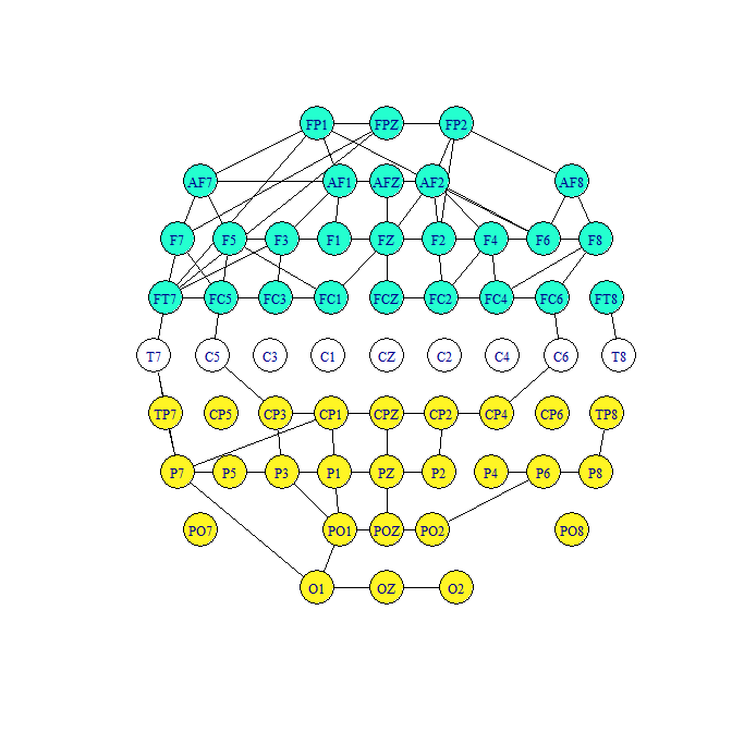
Figure 5: Estimated brain connectivity results from SyGlasso for (a) the alcoholic subject and (b) the control subject. The blue nodes correspond to the frontal region, and the yellow nodes correspond to the parietal and occipital regions. The alcoholic subject has asymmetric brain connections in the frontal region compared to the control subject.

Figure 5 shows the result of the SyGlasso estimated network of electrodes. For comparison, both graphs were thresholded to match 5% sparsity level. Similar to the findings of Qiao et al., 2019, our estimated graph 𝚿n​o​d​e\bm{\Psi}_{node} for the alcoholic group shows the asymmetry between the left and the right side of the brain compared to the more balanced control group. Our finding is also consistent with the result in Hayden et al., 2006 and Zhu et al., 2016 that showed frontal asymmetry of the alcoholic subjects.

Refer to caption
(a) Alcoholic subject
Refer to caption
(b) Control subject
Figure 6: Support (off-diagonals) of SyGlasso-estimated temporal Sylvester factor 𝚿^t​i​m​e\hat{\mathbf{\Psi}}_{time} of the precision matrix for (a) the alcoholic subject and (b) the control subject. Both subjects exhibit banded conditional dependency structures over time.

While previous analyses on this EEG data using graphical models only focused on the precision matrix of the electrodes, here we exhibit in Figure 6 the second precision matrix that encodes temporal dependency. Overall both subjects exhibit banded dependency structures over time, since adjacent timepoints are conditionally dependent. However, note that the conditional dependency structure of the timepoints for the alcoholic subject appears to be more chaotic.

6 Discussion

This paper proposed Sylvester-structured graphical model and an inference algorithm, the SyGlasso, that can be applied to tensor-valued data. The current tools available for researchers are limited to Kronecker product and Kronecker sum models on either the covariance or the precision matrix. Our model is motivated by a generative stochastic representation based on the Sylvester equation. We showed that the resulting precision matrix corresponds to the squared Kronecker sum of the precision matrices 𝚿k\mathbf{\Psi}_{k} along each mode. The individual components 𝚿k\mathbf{\Psi}_{k}’s are estimated by the nodewise regression based approach.

There are several promising future directions to take the proposed SyGlasso. First is to relax the assumption that the diagonals of the factors are fixed - an assumption that is standard among the Kronecker structured models for theoretical analysis. Practically, SyGlasso is able to recover the off-diagonals of the individual 𝚿k\bm{\Psi}_{k} and the diagonal of 𝛀\bm{\Omega}, which only requires to estimating ⨁k=1Kdiag​(𝚿k)\bigoplus_{k=1}^{K}\text{diag}(\bm{\Psi}_{k}) instead of all diagonal entries diag​(𝚿𝒌)\text{diag}(\bm{\Psi_{k}}) for all kk. However, we believe that analyzing the sparsity pattern of the squared Kronecker sum matrix would help us estimate the diagonal entries of the individual components 𝚿k\mathbf{\Psi}_{k}’s. In addition, it would be worthwhile to study optimization procedures that perform matrix-wise estimation of 𝚿k\bm{\Psi}_{k} (yielding simultaneous estimates for both off-diagonal and diagonal entries) and compare its empirical and theoretical properties with the approach proposed in this paper.

Secondly, in terms of the statistical properties, our theoretical results guarantee sparsistency of the individual graphs with a slower convergence rate than that is proposed in Greenewald et al., 2019, while empirical evidence suggests that a faster rate can be achieved. Improvement of this statistical convergence rate analysis will be worthwhile. Also, our results do not guarantee the statistical convergence of individual 𝚿k\mathbf{\Psi}_{k}’s nor 𝛀\bm{\Omega} with respect to the operator norm. Similar to the solution proposed in Zhou et al., 2011, we plan to adopt a two-step procedure using SyGlasso for variable selection followed by refitting the precision matrix 𝛀\mathbf{\Omega} using maximum likelihood estimation with edge constraint.

Lastly, an exciting future direction is to investigate the utility of SyGlasso as a tool to perform system identification for systems that can be modeled by Sylvester approximations to differential equations. Such dynamical systems include, for example, physical processes governed by separable elliptic PDEs as described in Grasedyck, 2004, Kressner and Tobler, 2010. It is likely that myriad physical processes can be well-modeled using a Sylvester equation, leading to sparse precision matrices (e.g., a space-time process satisfying the Poisson equation).

Acknowledgments

The authors acknowledge US agency support by grants ARO W911NF-15-1-0479 and DOE DE-NA0003921.

References

  • Bai et al., (2003) Bai, Z.-Z., Golub, G. H., and Ng, M. K. (2003). Hermitian and skew-hermitian splitting methods for non-hermitian positive definite linear systems. SIAM Journal on Matrix Analysis and Applications, 24(3):603–626.
  • Besag, (1977) Besag, J. (1977). Efficiency of pseudolikelihood estimation for simple gaussian fields. Biometrika, pages 616–618.
  • Datta and Zou, (2017) Datta, A. and Zou, H. (2017). Cocolasso for high-dimensional error-in-variables regression. The Annals of Statistics, 45(6):2400–2426.
  • Dawid, (1981) Dawid, A. P. (1981). Some matrix-variate distribution theory: notational considerations and a bayesian application. Biometrika, 68(1):265–274.
  • Friedman et al., (2008) Friedman, J., Hastie, T., and Tibshirani, R. (2008). Sparse inverse covariance estimation with the graphical lasso. Biostatistics, 9(3):432–441.
  • Friedman et al., (2010) Friedman, J., Hastie, T., and Tibshirani, R. (2010). Applications of the lasso and grouped lasso to the estimation of sparse graphical models. Technical report, Technical report, Stanford University.
  • Grasedyck, (2004) Grasedyck, L. (2004). Existence and computation of low kronecker-rank approximations for large linear systems of tensor product structure. Computing, 72(3-4):247–265.
  • Greenewald et al., (2019) Greenewald, K., Zhou, S., and Hero III, A. (2019). Tensor graphical lasso (teralasso). To appear in JRSS-B. arXiv preprint arXiv:1705.03983.
  • Hayden et al., (2006) Hayden, E. P., Wiegand, R. E., Meyer, E. T., Bauer, L. O., O’Connor, S. J., Nurnberger Jr, J. I., Chorlian, D. B., Porjesz, B., and Begleiter, H. (2006). Patterns of regional brain activity in alcohol-dependent subjects. Alcoholism: Clinical and Experimental Research, 30(12):1986–1991.
  • Kalaitzis et al., (2013) Kalaitzis, A., Lafferty, J., Lawrence, N. D., and Zhou, S. (2013). The bigraphical lasso. In International Conference on Machine Learning, pages 1229–1237.
  • Khare et al., (2015) Khare, K., Oh, S.-Y., and Rajaratnam, B. (2015). A convex pseudolikelihood framework for high dimensional partial correlation estimation with convergence guarantees. Journal of the Royal Statistical Society: Series B (Statistical Methodology), 77(4):803–825.
  • Khare and Rajaratnam, (2014) Khare, K. and Rajaratnam, B. (2014). Convergence of cyclic coordinatewise l1 minimization. arXiv preprint arXiv:1404.5100.
  • Knyazev, (2007) Knyazev, G. G. (2007). Motivation, emotion, and their inhibitory control mirrored in brain oscillations. Neuroscience & Biobehavioral Reviews, 31(3):377–395.
  • Kolda and Bader, (2009) Kolda, T. G. and Bader, B. W. (2009). Tensor decompositions and applications. SIAM review, 51(3):455–500.
  • Kressner and Tobler, (2010) Kressner, D. and Tobler, C. (2010). Krylov subspace methods for linear systems with tensor product structure. SIAM journal on matrix analysis and applications, 31(4):1688–1714.
  • Lyu et al., (2019) Lyu, X., Sun, W. W., Wang, Z., Liu, H., Yang, J., and Cheng, G. (2019). Tensor graphical model: Non-convex optimization and statistical inference. IEEE transactions on pattern analysis and machine intelligence.
  • Matthews, (1975) Matthews, B. W. (1975). Comparison of the predicted and observed secondary structure of t4 phage lysozyme. Biochimica et Biophysica Acta (BBA)-Protein Structure, 405(2):442–451.
  • Meinshausen and Bühlmann, (2006) Meinshausen, N. and Bühlmann, P. (2006). High-dimensional graphs and variable selection with the lasso. The Annals of Statistics, pages 1436–1462.
  • Park et al., (2017) Park, S., Shedden, K., and Zhou, S. (2017). Non-separable covariance models for spatio-temporal data, with applications to neural encoding analysis. arXiv preprint arXiv:1705.05265.
  • Peng et al., (2009) Peng, J., Wang, P., Zhou, N., and Zhu, J. (2009). Partial correlation estimation by joint sparse regression models. Journal of the American Statistical Association, 104(486):735–746.
  • Qiao et al., (2019) Qiao, X., Guo, S., and James, G. M. (2019). Functional graphical models. Journal of the American Statistical Association, 114(525):211–222.
  • Rudelson and Zhou, (2017) Rudelson, M. and Zhou, S. (2017). Errors-in-variables models with dependent measurements. Electronic Journal of Statistics, 11(1):1699–1797.
  • Tsiligkaridis et al., (2013) Tsiligkaridis, T., Hero III, A. O., and Zhou, S. (2013). On convergence of kronecker graphical lasso algorithms. IEEE transactions on signal processing, 61(7):1743–1755.
  • Varin et al., (2011) Varin, C., Reid, N., and Firth, D. (2011). An overview of composite likelihood methods. Statistica Sinica, pages 5–42.
  • Zhang et al., (1995) Zhang, X. L., Begleiter, H., Porjesz, B., Wang, W., and Litke, A. (1995). Event related potentials during object recognition tasks. Brain Research Bulletin, 38(6):531–538.
  • Zhao and Yu, (2006) Zhao, P. and Yu, B. (2006). On model selection consistency of lasso. Journal of Machine learning research, 7(Nov):2541–2563.
  • Zhou, (2014) Zhou, S. (2014). GEMINI: Graph estimation with matrix variate normal instances. The Annals of Statistics, 42(2):532–562.
  • Zhou et al., (2011) Zhou, S., Rütimann, P., Xu, M., and Bühlmann, P. (2011). High-dimensional covariance estimation based on gaussian graphical models. Journal of Machine Learning Research, 12(Oct):2975–3026.
  • Zhu et al., (2016) Zhu, H., Strawn, N., and Dunson, D. B. (2016). Bayesian graphical models for multivariate functional data. The Journal of Machine Learning Research, 17(1):7157–7183.

Appendix

  • A provides the detailed derivation of the updates for Algorithm 1.

  • B provides the proofs of theorems stated in Section 3.

  • C provides details on the simulated data in Section 4.

Appendix A Derivation of the Nodewise Tensor Lasso Estimator

A.1 Off-Diagonal updates

For 1≤ik<jk≤mk1\leq i_{k}<j_{k}\leq m_{k}, Tik​jk​(𝚿koff)T_{i_{k}j_{k}}(\mathbf{\Psi}_{k}^{\text{off}}) can be computed in closed form:

(Tik​jk​(𝚿k))ik​jkoff=SλkN​(F𝓧,{𝚿k}k=1K)(1N​𝓧(k)​𝓧(k)T)ik​ik+(1N​𝓧(k)​𝓧(k)T)jk​jk,(T_{i_{k}j_{k}}(\mathbf{\Psi}_{k}))_{i_{k}j_{k}}^{\text{off}}=\frac{S_{\frac{\lambda_{k}}{N}}\Big(F_{\bm{\mathcal{X}},\{\mathbf{\Psi}_{k}\}_{k=1}^{K}}\Big)}{(\frac{1}{N}\bm{\mathcal{X}}_{(k)}\bm{\mathcal{X}}_{(k)}^{T})_{i_{k}i_{k}}+(\frac{1}{N}\bm{\mathcal{X}}_{(k)}\bm{\mathcal{X}}_{(k)}^{T})_{j_{k}j_{k}}}, (9)

where

F𝓧,{𝚿k}k=1K=−1N\displaystyle F_{\bm{\mathcal{X}},\{\mathbf{\Psi}_{k}\}_{k=1}^{K}}=-\frac{1}{N} (((𝓦(k)∘𝓧(k))​𝓧(k)T)ik​jk+((𝓦(k)∘𝓧(k))​𝓧(k)T)jk​ikCLOSE\displaystyle\Bigg(\Big((\bm{\mathcal{W}}_{(k)}\circ\bm{\mathcal{X}}_{(k)})\bm{\mathcal{X}}_{(k)}^{T}\Big)_{i_{k}j_{k}}+\Big((\bm{\mathcal{W}}_{(k)}\circ\bm{\mathcal{X}}_{(k)})\bm{\mathcal{X}}_{(k)}^{T}\Big)_{j_{k}i_{k}}
+(𝓧(k)​(𝓧×k𝚿koff,ik​jk)(k)T)jk​ik+(𝓧(k)​(𝓧×k𝚿koff,ik​jk)(k)T)ik​jk\displaystyle+\Big(\bm{\mathcal{X}}_{(k)}(\bm{\mathcal{X}}\times_{k}\mathbf{\Psi}_{k}^{\text{off},i_{k}j_{k}})^{T}_{(k)}\Big)_{j_{k}i_{k}}+\Big(\bm{\mathcal{X}}_{(k)}(\bm{\mathcal{X}}\times_{k}\mathbf{\Psi}_{k}^{\text{off},i_{k}j_{k}})^{T}_{(k)}\Big)_{i_{k}j_{k}}
+∑l≠k(𝓧(k)(𝓧×l𝚿loff)(k)T)ik​jk+∑l≠k(𝓧(k)(𝓧×l𝚿loff)(k)T)jk​ik).\displaystyle\quad+\sum_{l\neq k}\Big(\bm{\mathcal{X}}_{(k)}(\bm{\mathcal{X}}\times_{l}\mathbf{\Psi}_{l}^{\text{off}})^{T}_{(k)}\Big)_{i_{k}j_{k}}+\sum_{l\neq k}\Big(\bm{\mathcal{X}}_{(k)}(\bm{\mathcal{X}}\times_{l}\mathbf{\Psi}_{l}^{\text{off}})^{T}_{(k)}\Big)_{j_{k}i_{k}}\Bigg).

Here the ∘\circ operator denotes the Hadamard product between matrices; 𝚿koff,ik​jk\mathbf{\Psi}_{k}^{\text{off},i_{k}j_{k}} is 𝚿koff\mathbf{\Psi}_{k}^{\text{off}} with the (ik,jk)(i_{k},j_{k}) entry being zero; and Sλ​(x):=sign​(x)​(|x|−λ)+S_{\lambda}(x):=\text{sign}(x)(|x|-\lambda)_{+} is the soft-thresholding operator.

A.2 Diagonal updates

For 𝓦\bm{\mathcal{W}},

(T(𝓦))i[1:K]=−(𝓧(N)T𝓨(N))i[1:K]+(𝓧(N)T𝓨(N))i[1:K]2+4(𝓧(N)𝓧(N)T)i[1:K]2(𝓧(N)𝓧(N)T)i[1:K].(T(\bm{\mathcal{W}}))_{i_{[1:K]}}=\frac{-\Big(\bm{\mathcal{X}}_{(N)}^{T}\bm{\mathcal{Y}}_{(N)}\Big)_{i_{[1:K]}}+\sqrt{\Big(\bm{\mathcal{X}}_{(N)}^{T}\bm{\mathcal{Y}}_{(N)}\Big)_{i_{[1:K]}}^{2}+4\Big(\bm{\mathcal{X}}_{(N)}\bm{\mathcal{X}}_{(N)}^{T}\Big)_{i_{[1:K]}}}}{2\Big(\bm{\mathcal{X}}_{(N)}\bm{\mathcal{X}}_{(N)}^{T}\Big)_{i_{[1:K]}}}. (10)

Here we define 𝓨:=∑k=1K(𝓧×k𝚿koff)\bm{\mathcal{Y}}:=\sum_{k=1}^{K}\Big(\bm{\mathcal{X}}\times_{k}\mathbf{\Psi}_{k}^{\text{off}}\Big). Equations (9) and (10) give necessary ingredients for designing a coordinate descent approach to minimizing the objective function in (4). The optimization procedure is summarized in Algorithm 1.

A.3 Derivation of updates

Note that for 1≤ik<jk≤mk1\leq i_{k}<j_{k}\leq m_{k}, 1≤k≤K1\leq k\leq K,

QN​({𝚿k}k=1K)\displaystyle Q_{N}(\{\mathbf{\Psi}_{k}\}_{k=1}^{K})
=(N/2)(∑i[1:k−1,k+1:K](𝓧i[1:K]ik2+𝓧i[1:K]jk2))((𝚿k)ik​jk)2\displaystyle=(N/2)\Big(\sum_{i_{[1:k-1,k+1:K]}}({\bm{\mathcal{X}}_{i_{[1:K]}}^{i_{k}}}^{2}+{\bm{\mathcal{X}}_{i_{[1:K]}}^{j_{k}}}^{2})\Big)\Big((\mathbf{\Psi}_{k})_{i_{k}j_{k}}\Big)^{2}
+N​F𝓧,{𝚿}k=1K​(𝚿k)ik​jk+λk​|(𝚿k)ik​jk|\displaystyle+NF_{\bm{\mathcal{X}},\{\mathbf{\Psi}\}_{k=1}^{K}}(\mathbf{\Psi}_{k})_{i_{k}j_{k}}+\lambda_{k}|(\mathbf{\Psi}_{k})_{i_{k}j_{k}}|
+terms independent of (𝚿k)ik​jk,\displaystyle+\text{terms independent of $(\mathbf{\Psi}_{k})_{i_{k}j_{k}}$},

where

F𝓧,{𝚿}k=1K=−∑i[1:k−1,k+1:K]\displaystyle F_{\bm{\mathcal{X}},\{\mathbf{\Psi}\}_{k=1}^{K}}=-\sum_{i_{[1:k-1,k+1:K]}} (𝓦i[1:K]ik𝓧i[1:K]ik𝓧i[1:K]jk+𝓦i[1:K]jk𝓧i[1:K]jk𝓧i[1:K]ik\displaystyle\Big(\bm{\mathcal{W}}_{i_{[1:K]}}^{i_{k}}\bm{\mathcal{X}}_{i_{[1:K]}}^{i_{k}}\bm{\mathcal{X}}_{i_{[1:K]}}^{j_{k}}+\bm{\mathcal{W}}_{i_{[1:K]}}^{j_{k}}\bm{\mathcal{X}}_{i_{[1:K]}}^{j_{k}}\bm{\mathcal{X}}_{i_{[1:K]}}^{i_{k}}
+(𝚿k)ik,\​{ik,jk}T𝓧i[1:K]\​{ik,jk}𝓧i[1:K]jk\displaystyle+(\mathbf{\Psi}_{k})_{i_{k},\text{\textbackslash}\{i_{k},j_{k}\}}^{T}\bm{\mathcal{X}}_{i_{[1:K]}}^{\text{\textbackslash}\{i_{k},j_{k}\}}\bm{\mathcal{X}}_{i_{[1:K]}}^{j_{k}}
+(𝚿k)jk,\​{ik,jk}T𝓧i[1:K]\​{ik,jk}𝓧i[1:K]ik\displaystyle+(\mathbf{\Psi}_{k})_{j_{k},\text{\textbackslash}\{i_{k},j_{k}\}}^{T}\bm{\mathcal{X}}_{i_{[1:K]}}^{\text{\textbackslash}\{i_{k},j_{k}\}}\bm{\mathcal{X}}_{i_{[1:K]}}^{i_{k}}
+∑l∈[1:k−1,k+1:K](𝚿l)il,\​ilT𝓧i[1:K]ik,\​il𝓧i[1:K]jk\displaystyle+\sum_{l\in[1:k-1,k+1:K]}(\mathbf{\Psi}_{l})_{i_{l},\text{\textbackslash}i_{l}}^{T}\bm{\mathcal{X}}_{i_{[1:K]}}^{i_{k},\text{\textbackslash}i_{l}}\bm{\mathcal{X}}_{i_{[1:K]}}^{j_{k}}
+∑l∈[1:k−1,k+1:K](𝚿l)il,\​ilT𝓧i[1:K]jk,\​il𝓧i[1:K]ik).\displaystyle+\sum_{l\in[1:k-1,k+1:K]}(\mathbf{\Psi}_{l})_{i_{l},\text{\textbackslash}i_{l}}^{T}\bm{\mathcal{X}}_{i_{[1:K]}}^{j_{k},\text{\textbackslash}i_{l}}\bm{\mathcal{X}}_{i_{[1:K]}}^{i_{k}}\Big).

Here 𝓧i[1:K]ik\bm{\mathcal{X}}_{i_{[1:K]}}^{i_{k}} denotes the element of 𝓧\bm{\mathcal{X}} indexed by i[1:K]i_{[1:K]} except that the kkth index is replaced by iki_{k} and 𝓧i[1:K]ik,jl\bm{\mathcal{X}}_{i_{[1:K]}}^{i_{k},j_{l}} denotes the element of 𝓧\bm{\mathcal{X}} indexed by i[1:K]i_{[1:K]} except that the k,lk,lth indices are replaced by ik,jli_{k},j_{l}. Note the following equivalence:

∑i[1:k−1,k+1:K]𝓦i[1:K]ik𝓧i[1:K]ik𝓧i[1:K]jk=((𝓦(k)∘𝓧(k))𝓧(k)T)ik​jk\displaystyle\sum_{i_{[1:k-1,k+1:K]}}\bm{\mathcal{W}}_{i_{[1:K]}}^{i_{k}}\bm{\mathcal{X}}_{i_{[1:K]}}^{i_{k}}\bm{\mathcal{X}}_{i_{[1:K]}}^{j_{k}}=\Big((\bm{\mathcal{W}}_{(k)}\circ\bm{\mathcal{X}}_{(k)})\bm{\mathcal{X}}_{(k)}^{T}\Big)_{i_{k}j_{k}}
∑i[1:k−1,k+1:K]𝓧i[1:K]ik𝓧i[1:K]jk=(𝓧(k)𝓧(k)T)ik​jk\displaystyle\sum_{i_{[1:k-1,k+1:K]}}\bm{\mathcal{X}}_{i_{[1:K]}}^{i_{k}}\bm{\mathcal{X}}_{i_{[1:K]}}^{j_{k}}=(\bm{\mathcal{X}}_{(k)}\bm{\mathcal{X}}_{(k)}^{T})_{i_{k}j_{k}}
∑i[1:k−1,k+1:K](𝚿l)il,.T𝓧i[1:K]ik,.𝓧i[1:K]jk=(𝓧(k)(𝓧×l𝚿l)(k)T)jk​ik,\displaystyle\sum_{i_{[1:k-1,k+1:K]}}(\mathbf{\Psi}_{l})_{i_{l},.}^{T}\bm{\mathcal{X}}_{i_{[1:K]}}^{i_{k},.}\bm{\mathcal{X}}_{i_{[1:K]}}^{j_{k}}=\Big(\bm{\mathcal{X}}_{(k)}(\bm{\mathcal{X}}\times_{l}\mathbf{\Psi}_{l})_{(k)}^{T}\Big)_{j_{k}i_{k}},

where 𝓦\bm{\mathcal{W}} is a tensor of the same dimensions of 𝓧\bm{\mathcal{X}}, formed by tensorize values in 𝓦\bm{\mathcal{W}}, and in the case of N>1N>1 the last mode of 𝓦\bm{\mathcal{W}} is the observation mode similarly to 𝓧\bm{\mathcal{X}} but with exact replicates. Using the tensor notation and standard sub-differential method, Equation (9) then follows.

For 𝓦i[1:K]\bm{\mathcal{W}}_{i_{[1:K]}}, using similar tensor operations,

∂∂𝓦i[1:K]QN(𝓦,{𝚿koff}k=1K)=0\displaystyle\frac{\partial}{\partial\bm{\mathcal{W}}_{i_{[1:K]}}}Q_{N}(\bm{\mathcal{W}},\{\mathbf{\Psi}_{k}^{\text{off}}\}_{k=1}^{K})=0
⇔−1𝓦i[1:K]+𝓦i[1:K]2𝓧i[1:K]2+𝓦i[1:K](𝓧i[1:K]∑k=1K(𝓧×k𝚿koff)i[1:K]))=0\displaystyle\iff-\frac{1}{\bm{\mathcal{W}}_{i_{[1:K]}}}+\bm{\mathcal{W}}_{i_{[1:K]}}^{2}\bm{\mathcal{X}}_{i_{[1:K]}}^{2}+\bm{\mathcal{W}}_{i_{[1:K]}}\Big(\bm{\mathcal{X}}_{i_{[1:K]}}\sum_{k=1}^{K}(\bm{\mathcal{X}}\times_{k}\mathbf{\Psi}_{k}^{\text{off}})_{i_{[1:K]}})\Big)=0
⇔𝓦i[1:K]2(𝓧(N)T𝓧(N))i[1:K]+𝓦i[1:K](𝓧(N)T∑k=1K(𝓧×k𝚿koff))i[1:K]−1=0\displaystyle\iff\bm{\mathcal{W}}_{i_{[1:K]}}^{2}\Big(\bm{\mathcal{X}}_{(N)}^{T}\bm{\mathcal{X}}_{(N)}\Big)_{i_{[1:K]}}+\bm{\mathcal{W}}_{i_{[1:K]}}\Big(\bm{\mathcal{X}}_{(N)}^{T}\sum_{k=1}^{K}(\bm{\mathcal{X}}\times_{k}\mathbf{\Psi}_{k}^{\text{off}})\Big)_{i_{[1:K]}}-1=0

which is a quadratic equation in 𝓦i[1:K]\bm{\mathcal{W}}_{i_{[1:K]}} and since 𝓦i[1:K]>0\bm{\mathcal{W}}_{i_{[1:K]}}>0, so the positive root has been retained as the solution. Note that the estimation for one entry of 𝓦\bm{\mathcal{W}} is independent of the other entries. So during the estimation process we update all the entries at once by noting that diag(𝓧(N)T𝓧(N))=((𝓧(N)T𝓧(N))i[1:K],∀i[1:K])\mathop{\text{diag}}\Big(\bm{\mathcal{X}}_{(N)}^{T}\bm{\mathcal{X}}_{(N)}\Big)=\Big(\Big(\bm{\mathcal{X}}_{(N)}^{T}\bm{\mathcal{X}}_{(N)}\Big)_{i_{[1:K]}},\forall i_{[1:K]}\Big).

Appendix B Proofs of Main Theorems

We first list some properties of the loss function.

Lemma B.1.

The following is true for the loss function:

  1. (i)

    There exist constants 0<ΛminL≤ΛmaxL<∞0<\Lambda_{\min}^{L}\leq\Lambda_{\max}^{L}<\infty such that for 𝒮k:={(ik,jk):1≤ik<jk≤mk},k=1,…,K\mathcal{S}_{k}:=\{(i_{k},j_{k}):1\leq i_{k}<j_{k}\leq m_{k}\},k=1,\dots,K,

    ΛminL≤λmin​(L¯𝒮k,𝒮k′′​(𝜷¯))≤λmax​(L¯𝒮k,𝒮k′′​(𝜷¯))≤ΛmaxL\Lambda_{\min}^{L}\leq\lambda_{\min}(\bar{L}^{\prime\prime}_{\mathcal{S}_{k},\mathcal{S}_{k}}(\bar{\bm{\beta}}))\leq\lambda_{\max}(\bar{L}^{\prime\prime}_{\mathcal{S}_{k},\mathcal{S}_{k}}(\bar{\bm{\beta}}))\leq\Lambda_{\max}^{L}
  2. (ii)

    There exists a constant K⁡(𝜷¯)<∞K(\bar{\bm{\beta}})<\infty such that for all 1≤ik<jk≤mk1\leq i_{k}<j_{k}\leq m_{k}, L¯ik​jk,ik​jk′′​(𝜷¯)≤K⁡(𝜷¯)\bar{L}^{\prime\prime}_{i_{k}j_{k},i_{k}j_{k}}(\bar{\bm{\beta}})\leq K(\bar{\bm{\beta}})

  3. (iii)

    There exist constant M1​(𝜷¯),M2​(𝜷¯)<∞M_{1}(\bar{\bm{\beta}}),M_{2}(\bar{\bm{\beta}})<\infty, such that for any 1≤ik<jk≤mk1\leq i_{k}<j_{k}\leq m_{k}

    Var𝓦¯,𝜷¯⁡(Lik​jk′​(𝓦¯,𝜷¯,𝓧))≤M1​(𝜷¯),Var𝓦¯,𝜷¯⁡(Lik​jk,ik​jk′′​(𝓦¯,𝜷¯,𝓧))≤M2​(𝜷¯)\Var_{\bar{\bm{\mathcal{W}}},\bar{\bm{\beta}}}(L^{\prime}_{i_{k}j_{k}}(\bar{\bm{\mathcal{W}}},\bar{\bm{\beta}},\bm{\mathcal{X}}))\leq M_{1}(\bar{\bm{\beta}}),\ \Var_{\bar{\bm{\mathcal{W}}},\bar{\bm{\beta}}}(L^{\prime\prime}_{i_{k}j_{k},i_{k}j_{k}}(\bar{\bm{\mathcal{W}}},\bar{\bm{\beta}},\bm{\mathcal{X}}))\leq M_{2}(\bar{\bm{\beta}})
  4. (iv)

    There exists a constant 0<g⁡(𝜷¯)<∞0<g(\bar{\bm{\beta}})<\infty, such that for all (i,j)∈𝒜k(i,j)\in\mathcal{A}_{k}

    L¯i​j,i​j′′​(𝓦¯,𝜷¯)−L¯i​j,𝒜ki​j′′​(𝓦¯,𝜷¯)​[L¯𝒜ki​j,𝒜ki​j′′​(𝓦¯,𝜷¯)]−1​L¯𝒜ki​j,i​j′′​(𝓦¯,𝜷¯)≥g⁡(𝜷¯),\bar{L}^{\prime\prime}_{ij,ij}(\bar{\bm{\mathcal{W}}},\bar{\bm{\beta}})-\bar{L}^{\prime\prime}_{ij,\mathcal{A}_{k}^{ij}}(\bar{\bm{\mathcal{W}}},\bar{\bm{\beta}})[\bar{L}^{\prime\prime}_{\mathcal{A}_{k}^{ij},\mathcal{A}_{k}^{ij}}(\bar{\bm{\mathcal{W}}},\bar{\bm{\beta}})]^{-1}\bar{L}^{\prime\prime}_{\mathcal{A}_{k}^{ij},ij}(\bar{\bm{\mathcal{W}}},\bar{\bm{\beta}})\geq g(\bar{\bm{\beta}}),

    where 𝒜ki​j:=𝒜k/{(i,j)}\mathcal{A}_{k}^{ij}:=\mathcal{A}_{k}/\{(i,j)\}.

  5. (v)

    There exists a constant M⁡(𝜷¯)<∞M(\bar{\bm{\beta}})<\infty, such that for any (i,j)∈𝒜kc(i,j)\in\mathcal{A}_{k}^{c}

    ‖L¯i​j,𝒜k′′​(𝓦¯,𝜷¯)​[L¯𝒜k,𝒜k′′​(𝓦¯,𝜷¯)]−1‖2≤M⁡(𝜷¯).\|\bar{L}^{\prime\prime}_{ij,\mathcal{A}_{k}}(\bar{\bm{\mathcal{W}}},\bar{\bm{\beta}})[\bar{L}^{\prime\prime}_{\mathcal{A}_{k},\mathcal{A}_{k}}(\bar{\bm{\mathcal{W}}},\bar{\bm{\beta}})]^{-1}\|_{2}\leq M(\bar{\bm{\beta}}).
proof of Lemma B.1.

We prove (i)(i). (i​i−v)(ii-v) are then direct consequences, and the proofs follow from the proofs of B1.1-B1.4 in Peng et al., 2009, with the modifications being that the indexing is now with respect to each kk for 1≤k≤K1\leq k\leq K.

Consider the loss function in matrix form as in (2). Then L¯𝒮k,𝒮k′′​(𝜷¯)\bar{L}^{\prime\prime}_{\mathcal{S}_{k},\mathcal{S}_{k}}(\bar{\bm{\beta}}) is equivalent to ∂2∂𝚿koff​∂𝚿koff​L​(𝓦,{𝚿koff}k=1K)\frac{\partial^{2}}{\partial\mathbf{\Psi}_{k}^{\text{off}}\partial\mathbf{\Psi}_{k}^{\text{off}}}L(\bm{\mathcal{W}},\{\mathbf{\Psi}_{k}^{\text{off}}\}_{k=1}^{K}), which is

∂2∂𝚿koff​∂𝚿koff​(tr(𝚿kT​𝐒​𝚿k)+first order terms in 𝚿k+terms independent of 𝚿k)\displaystyle\frac{\partial^{2}}{\partial\mathbf{\Psi}_{k}^{\text{off}}\partial\mathbf{\Psi}_{k}^{\text{off}}}\Bigg(\tr(\mathbf{\Psi}_{k}^{T}\mathbf{S}\mathbf{\Psi}_{k})+\text{first order terms in $\mathbf{\Psi}_{k}$}+\text{terms independent of $\mathbf{\Psi}_{k}$}\Bigg)
=∂2∂𝚿koff​∂𝚿koff​(tr((𝚿koff+diag​(𝚿k))T​𝐒​(𝚿koff+diag​(𝚿k)))+first order terms in 𝚿koffCLOSE\displaystyle=\frac{\partial^{2}}{\partial\mathbf{\Psi}_{k}^{\text{off}}\partial\mathbf{\Psi}_{k}^{\text{off}}}\Bigg(\tr((\mathbf{\Psi}_{k}^{\text{off}}+\text{diag}(\mathbf{\Psi}_{k}))^{T}\mathbf{S}(\mathbf{\Psi}_{k}^{\text{off}}+\text{diag}(\mathbf{\Psi}_{k})))+\text{first order terms in $\mathbf{\Psi}_{k}^{\text{off}}$}
OPEN+terms independent of 𝚿koff)\displaystyle\qquad\qquad\qquad\quad+\text{terms independent of $\mathbf{\Psi}_{k}^{\text{off}}$}\Bigg)
=∂2∂𝚿koff​∂𝚿koff​(tr((𝚿koff)T​𝐒​𝚿koff)+first order terms in 𝚿koff+terms independent of 𝚿koff)\displaystyle=\frac{\partial^{2}}{\partial\mathbf{\Psi}_{k}^{\text{off}}\partial\mathbf{\Psi}_{k}^{\text{off}}}\Bigg(\tr((\mathbf{\Psi}_{k}^{\text{off}})^{T}\mathbf{S}\mathbf{\Psi}_{k}^{\text{off}})+\text{first order terms in $\mathbf{\Psi}_{k}^{\text{off}}$}+\text{terms independent of $\mathbf{\Psi}_{k}^{\text{off}}$}\Bigg)
=𝐒=1N​vec⁡(𝓧)T​vec⁡(𝓧).\displaystyle=\mathbf{S}=\frac{1}{N}\vecto(\bm{\mathcal{X}})^{T}\vecto(\bm{\mathcal{X}}).

Thus L¯𝒮k,𝒮k′′​(𝜷)=E𝓦,𝜷​(𝐒)\bar{L}^{\prime\prime}_{\mathcal{S}_{k},\mathcal{S}_{k}}(\bm{\beta})=E_{\bm{\mathcal{W}},\bm{\beta}}(\mathbf{S}). Then for any non-zero 𝐚∈ℝp\mathbf{a}\in\mathbb{R}^{p}, we have

𝐚T​L¯𝒮k,𝒮k′′​(𝜷¯)​𝐚=𝐚T​𝚺¯​𝐚≥‖𝐚‖22​λmin​(𝚺¯).\mathbf{a}^{T}\bar{L}^{\prime\prime}_{\mathcal{S}_{k},\mathcal{S}_{k}}(\bar{\bm{\beta}})\mathbf{a}=\mathbf{a}^{T}\mathbf{\bar{\Sigma}}\mathbf{a}\geq\|\mathbf{a}\|_{2}^{2}\lambda_{\min}(\bar{\mathbf{\Sigma}}).

Similarly, 𝐚T​L¯𝒮k,𝒮k′′​(𝜷¯)​𝐚≤‖𝐚‖22​λmax​(𝚺¯)\mathbf{a}^{T}\bar{L}^{\prime\prime}_{\mathcal{S}_{k},\mathcal{S}_{k}}(\bar{\bm{\beta}})\mathbf{a}\leq\|\mathbf{a}\|_{2}^{2}\lambda_{\max}(\bar{\mathbf{\Sigma}}). By (A2), 𝚺¯\bar{\mathbf{\Sigma}} has bounded eigenvalues, thus the lemma is proved.

∎

Lemma B.2.

Suppose conditions (A1-A2) hold, then for any η>0\eta>0, there exist constant c0,η,c1,η,c2,η,c3,ηc_{0,\eta},c_{1,\eta},c_{2,\eta},c_{3,\eta}, such that for any u∈ℝqku\in\mathbb{R}^{q_{k}} the following events hold with probability at least 1−O⁡(exp⁡(−η​log⁡p))1-O(\exp(-\eta\log p)) for sufficiently large NN:

  1. (i)

    ‖LN,𝒜k′​(𝓦¯,𝜷¯,𝓧)‖2≤c0,η​qk​log⁡pN\|L_{N,\mathcal{A}_{k}}^{\prime}(\bar{\bm{\mathcal{W}}},\bar{\bm{\beta}},\bm{\mathcal{X}})\|_{2}\leq c_{0,\eta}\sqrt{q_{k}\frac{\log p}{N}}

  2. (ii)

    |uT​LN,𝒜k′​(𝓦¯,𝜷¯,𝓧)|≤c1,η​‖u‖2​qk​log⁡pN|u^{T}L_{N,\mathcal{A}_{k}}^{\prime}(\bar{\bm{\mathcal{W}}},\bar{\bm{\beta}},\bm{\mathcal{X}})|\leq c_{1,\eta}\|u\|_{2}\sqrt{q_{k}\frac{\log p}{N}}

  3. (iii)

    |uT​LN,𝒜k​𝒜k′′​(𝓦¯,𝜷¯,𝓧)​u−uT​L¯𝒜k​𝒜k′′​(𝜷¯)​u|≤c2,η​‖u‖22​qk​log⁡pN|u^{T}L_{N,\mathcal{A}_{k}\mathcal{A}_{k}}^{\prime\prime}(\bar{\bm{\mathcal{W}}},\bar{\bm{\beta}},\bm{\mathcal{X}})u-u^{T}\bar{L}^{\prime\prime}_{\mathcal{A}_{k}\mathcal{A}_{k}}(\bar{\bm{\beta}})u|\leq c_{2,\eta}\|u\|_{2}^{2}q_{k}\sqrt{\frac{\log p}{N}}

  4. (iv)

    |LN,𝒜k​𝒜k′′​(𝓦¯,𝜷¯,𝓧)​u−L¯𝒜k​𝒜k′′​(𝜷¯)​u|≤c3,η​‖u‖22​qk​log⁡pN|L_{N,\mathcal{A}_{k}\mathcal{A}_{k}}^{\prime\prime}(\bar{\bm{\mathcal{W}}},\bar{\bm{\beta}},\bm{\mathcal{X}})u-\bar{L}^{\prime\prime}_{\mathcal{A}_{k}\mathcal{A}_{k}}(\bar{\bm{\beta}})u|\leq c_{3,\eta}\|u\|_{2}^{2}q_{k}\sqrt{\frac{\log p}{N}}

proof of Lemma B.2.

(i)(i) By Cauchy-Schwartz inequality,

‖LN,𝒜k′​(𝓦¯,𝜷¯,𝓧)‖2≤qk​maxi∈𝒜k​|LN,i′​(𝓦¯,𝜷¯,𝓧)|.\|L^{\prime}_{N,\mathcal{A}_{k}}(\bar{\bm{\mathcal{W}}},\bar{\bm{\beta}},\bm{\mathcal{X}})\|_{2}\leq\sqrt{q_{k}}\max_{i\in\mathcal{A}_{k}}|L^{\prime}_{N,i}(\bar{\bm{\mathcal{W}}},\bar{\bm{\beta}},\bm{\mathcal{X}})|.

Then note that

LN,i′​(𝓦,𝜷,𝓧)\displaystyle L^{\prime}_{N,i}(\bm{\mathcal{W}},\bm{\beta},\bm{\mathcal{X}})
=∑i[1:k−1,k+1:K](ei[1:k−1],p,i[k+1:K](𝓦,𝜷)𝓧i[1:k−1],q,i[k+1:K]+ei[1:k−1],q,i[k+1:K](𝓦,𝜷)𝓧i[1:k−1],p,i[k+1:K]),\displaystyle=\sum_{i_{[1:k-1,k+1:K]}}(e_{i_{[1:k-1]},p,i_{[k+1:K]}}(\bm{\mathcal{W}},\bm{\beta})\bm{\mathcal{X}}_{i_{[1:k-1]},q,i_{[k+1:K]}}+e_{i_{[1:k-1]},q,i_{[k+1:K]}}(\bm{\mathcal{W}},\bm{\beta})\bm{\mathcal{X}}_{i_{[1:k-1]},p,i_{[k+1:K]}}),

where ei[1:k−1],p,i[k+1:K]𝓧i[1:k−1],q,i[k+1:K](𝓦,𝜷)e_{i_{[1:k-1]},p,i_{[k+1:K]}}\bm{\mathcal{X}}_{i_{[1:k-1]},q,i_{[k+1:K]}}(\bm{\mathcal{W}},\bm{\beta}) is defined by

wi[1:k−1],p,i[k+1:K]𝓧i[1:k−1],p,i[k+1:K]+∑jk≠p(𝚿k)p,jk𝓧i[1:k−1],jk,i[k+1:K]+∑l≠k∑jl≠il(𝚿l)il,jl𝓧i[1:k−1],p,i[k+1:K].w_{i_{[1:k-1]},p,i_{[k+1:K]}}\bm{\mathcal{X}}_{i_{[1:k-1]},p,i_{[k+1:K]}}+\sum_{j_{k}\neq p}(\mathbf{\Psi}_{k})_{p,j_{k}}\bm{\mathcal{X}}_{i_{[1:k-1]},j_{k},i_{[k+1:K]}}+\sum_{l\neq k}\sum_{j_{l}\neq i_{l}}(\mathbf{\Psi}_{l})_{i_{l},j_{l}}\bm{\mathcal{X}}_{i_{[1:k-1]},p,i_{[k+1:K]}}.

Then evaluated at the true parameter values (𝓦¯,𝜷¯)(\bar{\bm{\mathcal{W}}},\bar{\bm{\beta}}), we have ei[1:k−1],p,i[k+1:K](𝓦¯,𝜷¯)e_{i_{[1:k-1]},p,i_{[k+1:K]}}(\bar{\bm{\mathcal{W}}},\bar{\bm{\beta}}) uncorrelated with 𝓧i[1:k−1],\p,i[k+1:K]\bm{\mathcal{X}}_{i_{[1:k-1]},\text{\textbackslash}p,i_{[k+1:K]}} and E(𝓦¯,𝜷¯)(ei[1:k−1],p,i[k+1:K](𝓦¯,𝜷¯))=0E_{(\bar{\bm{\mathcal{W}}},\bar{\bm{\beta}})}(e_{i_{[1:k-1]},p,i_{[k+1:K]}}(\bar{\bm{\mathcal{W}}},\bar{\bm{\beta}}))=0. Also, since 𝓧\bm{\mathcal{X}} is subgaussian and Var⁡(LN,i′​(𝓦¯,𝜷¯,𝓧))\Var(L^{\prime}_{N,i}(\bar{\bm{\mathcal{W}}},\bar{\bm{\beta}},\bm{\mathcal{X}})) is bounded by Lemma C.1. ∀i\forall i, LN,i′​(𝓦¯,𝜷¯,𝓧)L^{\prime}_{N,i}(\bar{\bm{\mathcal{W}}},\bar{\bm{\beta}},\bm{\mathcal{X}}) has subexponential tails. Thus, by Bernstein inequality,

P⁡(‖LN,𝒜k′​(𝓦¯,𝜷¯,𝓧)‖2≤c0,η​qk​log⁡pN)\displaystyle P(\|L_{N,\mathcal{A}_{k}}^{\prime}(\bar{\bm{\mathcal{W}}},\bar{\bm{\beta}},\bm{\mathcal{X}})\|_{2}\leq c_{0,\eta}\sqrt{q_{k}\frac{\log p}{N}})
≥P⁡(qk​maxi∈𝒜k​|LN,i′​(𝓦¯,𝜷¯,𝓧)|≤c0,η​qk​log⁡pN)≥1−O⁡(exp⁡(−η​log⁡p)).\displaystyle\geq P(\sqrt{q_{k}}\max_{i\in\mathcal{A}_{k}}|L^{\prime}_{N,i}(\bar{\bm{\mathcal{W}}},\bar{\bm{\beta}},\bm{\mathcal{X}})|\leq c_{0,\eta}\sqrt{q_{k}\frac{\log p}{N}})\geq 1-O(\exp(-\eta\log p)).

(i​i​i)(iii) By Cauchy-Schwartz,

|uT​LN,𝒜k​𝒜k′′​(𝓦¯,𝜷¯,𝓧)​u−uT​L¯𝒜k​𝒜k′′​(𝜷¯)​u|\displaystyle|u^{T}L_{N,\mathcal{A}_{k}\mathcal{A}_{k}}^{\prime\prime}(\bar{\bm{\mathcal{W}}},\bar{\bm{\beta}},\bm{\mathcal{X}})u-u^{T}\bar{L}^{\prime\prime}_{\mathcal{A}_{k}\mathcal{A}_{k}}(\bar{\bm{\beta}})u|
≤‖u‖2​‖uT​LN,𝒜k​𝒜k′′​(𝓦¯,𝜷¯,𝓧)−uT​L¯𝒜k​𝒜k′′​(𝜷¯)‖2\displaystyle\leq\|u\|_{2}\|u^{T}L_{N,\mathcal{A}_{k}\mathcal{A}_{k}}^{\prime\prime}(\bar{\bm{\mathcal{W}}},\bar{\bm{\beta}},\bm{\mathcal{X}})-u^{T}\bar{L}^{\prime\prime}_{\mathcal{A}_{k}\mathcal{A}_{k}}(\bar{\bm{\beta}})\|_{2}
≤‖u‖2​qk​maxi​|uT​LN,𝒜k,i′′​(𝓦¯,𝜷¯,𝓧)−uT​L¯𝒜k,i′′​(𝜷¯)|\displaystyle\leq\|u\|_{2}\sqrt{q_{k}}\max_{i}|u^{T}L_{N,\mathcal{A}_{k},i}^{\prime\prime}(\bar{\bm{\mathcal{W}}},\bar{\bm{\beta}},\bm{\mathcal{X}})-u^{T}\bar{L}^{\prime\prime}_{\mathcal{A}_{k},i}(\bar{\bm{\beta}})|
=‖u‖2​qk​|uT​LN,𝒜k,imax′′​(𝓦¯,𝜷¯,𝓧)−uT​L¯𝒜k,imax′′​(𝜷¯)|\displaystyle=\|u\|_{2}\sqrt{q_{k}}|u^{T}L_{N,\mathcal{A}_{k},i_{\max}}^{\prime\prime}(\bar{\bm{\mathcal{W}}},\bar{\bm{\beta}},\bm{\mathcal{X}})-u^{T}\bar{L}^{\prime\prime}_{\mathcal{A}_{k},i_{\max}}(\bar{\bm{\beta}})|
=‖u‖2​qk​|∑j=1qk(uj​LN,j,imax′′​(𝓦¯,𝜷¯,𝓧)−uj​L¯j,imax′′​(𝜷¯))|\displaystyle=\|u\|_{2}\sqrt{q_{k}}|\sum_{j=1}^{q_{k}}(u_{j}L_{N,j,i_{\max}}^{\prime\prime}(\bar{\bm{\mathcal{W}}},\bar{\bm{\beta}},\bm{\mathcal{X}})-u_{j}\bar{L}^{\prime\prime}_{j,i_{\max}}(\bar{\bm{\beta}}))|
≤∥u∥2qk|ujmax||LN,jmax,imax′′(𝓦¯,𝜷¯,𝓧)−L¯jmax,imax′′(𝜷¯))|\displaystyle\leq\|u\|_{2}q_{k}|u_{j_{\max}}||L_{N,j_{\max},i_{\max}}^{\prime\prime}(\bar{\bm{\mathcal{W}}},\bar{\bm{\beta}},\bm{\mathcal{X}})-\bar{L}^{\prime\prime}_{j_{\max},i_{\max}}(\bar{\bm{\beta}}))|
≤∥u∥22qk|LN,jmax,imax′′(𝓦¯,𝜷¯,𝓧)−L¯jmax,imax′′(𝜷¯))|.\displaystyle\leq\|u\|_{2}^{2}q_{k}|L_{N,j_{\max},i_{\max}}^{\prime\prime}(\bar{\bm{\mathcal{W}}},\bar{\bm{\beta}},\bm{\mathcal{X}})-\bar{L}^{\prime\prime}_{j_{\max},i_{\max}}(\bar{\bm{\beta}}))|.

Then by Bernstein inequality,

P⁡(|uT​LN,𝒜k​𝒜k′′​(𝓦¯,𝜷¯,𝓧)​u−uT​L¯𝒜k​𝒜k′′​(𝜷¯)​u|≤c2,η​‖u‖22​qk​log⁡pN)\displaystyle P(|u^{T}L_{N,\mathcal{A}_{k}\mathcal{A}_{k}}^{\prime\prime}(\bar{\bm{\mathcal{W}}},\bar{\bm{\beta}},\bm{\mathcal{X}})u-u^{T}\bar{L}^{\prime\prime}_{\mathcal{A}_{k}\mathcal{A}_{k}}(\bar{\bm{\beta}})u|\leq c_{2,\eta}\|u\|_{2}^{2}q_{k}\sqrt{\frac{\log p}{N}})
OPEN≥P⁡(‖u‖22​qk|LN,jmax,imax′′​(𝓦¯,𝜷¯,𝓧)−L¯jmax,imax′′​(𝜷¯))|≤c2,η​‖u‖22​qk​log⁡pN)\displaystyle\geq P(\|u\|_{2}^{2}q_{k}|L_{N,j_{\max},i_{\max}}^{\prime\prime}(\bar{\bm{\mathcal{W}}},\bar{\bm{\beta}},\bm{\mathcal{X}})-\bar{L}^{\prime\prime}_{j_{\max},i_{\max}}(\bar{\bm{\beta}}))|\leq c_{2,\eta}\|u\|_{2}^{2}q_{k}\sqrt{\frac{\log p}{N}})
≥1−O⁡(exp⁡(−η​log⁡p)).\displaystyle\geq 1-O(\exp(-\eta\log p)).

(i​i)(ii) and (i​v)(iv) can be proved using similar arguments. ∎

Lemma C.3. and C.4. are used later to prove Theorem 1.

Lemma B.3.

Assuming conditions of Theorem 1. Then there exists a constant C1​(𝜷¯)>0C_{1}(\bar{\bm{\beta}})>0 such that for any η>0\eta>0, there exists a global minimizer of the restricted problem (8) within the disc:

{𝜷:‖𝜷−𝜷¯‖2≤C1​(𝜷¯)​K​maxk​qk​λN,k}\{\bm{\beta}:\|\bm{\beta}-\bar{\bm{\beta}}\|_{2}\leq C_{1}(\bar{\bm{\beta}})\sqrt{K}\max_{k}\sqrt{q_{k}}\lambda_{N,k}\}

with probability at least 1−O⁡(exp⁡(−η​log⁡p))1-O(\exp(-\eta\log p)) for sufficiently large NN.

proof of Lemma B.3.

Let αN=maxk⁡qk​λN,k\alpha_{N}=\max_{k}\sqrt{q_{k}}\lambda_{N,k}. Further for 1≤k≤K1\leq k\leq K let Ck>0C_{k}>0 and uk∈ℝmk​(mk−1)/2u^{k}\in\mathbb{R}^{m_{k}(m_{k}-1)/2} such that u𝒜kck=0u_{\mathcal{A}_{k}^{c}}^{k}=0, ‖uk‖2=Ck\|u^{k}\|_{2}=C_{k}, and u=(u1,…,uK)u=(u_{1},\dots,u_{K}) with K​mink​Ck≤‖u‖2≤K​maxk​Ck\sqrt{K}\min_{k}C_{k}\leq\|u\|_{2}\leq\sqrt{K}\max_{k}C_{k}.

Then by Cauchy-Schwartz and triangle inequality, we have

‖𝜷¯k+αN​uk−αN​uk‖1≤‖𝜷¯k+αN​uk‖1+αN​‖uk‖1,\|\bar{\bm{\beta}}^{k}+\alpha_{N}u^{k}-\alpha_{N}u^{k}\|_{1}\leq\|\bar{\bm{\beta}}^{k}+\alpha_{N}u^{k}\|_{1}+\alpha_{N}\|u^{k}\|_{1},

and

‖𝜷¯k‖1−‖𝜷¯k+αN​uk‖1≤αN​‖uk‖1≤αN​qk​‖uk‖2=Ck​αN​qk.\|\bar{\bm{\beta}}^{k}\|_{1}-\|\bar{\bm{\beta}}^{k}+\alpha_{N}u^{k}\|_{1}\leq\alpha_{N}\|u^{k}\|_{1}\leq\alpha_{N}\sqrt{q_{k}}\|u^{k}\|_{2}=C_{k}\alpha_{N}\sqrt{q_{k}}.

Thus,

QN​(𝜷¯+αN​u,𝓧,{λN,k}k=1K)−QN​(𝜷¯,𝓧,{λN,k}k=1K)\displaystyle Q_{N}(\bar{\bm{\beta}}+\alpha_{N}u,\bm{\mathcal{X}},\{\lambda_{N,k}\}_{k=1}^{K})-Q_{N}(\bar{\bm{\beta}},\bm{\mathcal{X}},\{\lambda_{N,k}\}_{k=1}^{K})
=LN​(𝜷¯+αN​u,𝓧)−LN​(𝜷¯,𝓧)−∑k=1KλN,k​(‖𝜷¯k‖1−‖𝜷¯k+αN​uk‖1)\displaystyle=L_{N}(\bar{\bm{\beta}}+\alpha_{N}u,\bm{\mathcal{X}})-L_{N}(\bar{\bm{\beta}},\bm{\mathcal{X}})-\sum_{k=1}^{K}\lambda_{N,k}\big(\|\bar{\bm{\beta}}^{k}\|_{1}-\|\bar{\bm{\beta}}^{k}+\alpha_{N}u^{k}\|_{1}\big)
≥LN​(𝜷¯+αN​u,𝓧)−LN​(𝜷¯,𝓧)−∑k=1KλN,k​Ck​αN​qk\displaystyle\geq L_{N}(\bar{\bm{\beta}}+\alpha_{N}u,\bm{\mathcal{X}})-L_{N}(\bar{\bm{\beta}},\bm{\mathcal{X}})-\sum_{k=1}^{K}\lambda_{N,k}C_{k}\alpha_{N}\sqrt{q_{k}}
≥LN​(𝜷¯+αN​u,𝓧)−LN​(𝜷¯,𝓧)−αN​K​maxk​Ck​qk​λN,k\displaystyle\geq L_{N}(\bar{\bm{\beta}}+\alpha_{N}u,\bm{\mathcal{X}})-L_{N}(\bar{\bm{\beta}},\bm{\mathcal{X}})-\alpha_{N}K\max_{k}C_{k}\sqrt{q_{k}}\lambda_{N,k}
≥LN​(𝜷¯+αN​u,𝓧)−LN​(𝜷¯,𝓧)−K​αN2​maxk​Ck.\displaystyle\geq L_{N}(\bar{\bm{\beta}}+\alpha_{N}u,\bm{\mathcal{X}})-L_{N}(\bar{\bm{\beta}},\bm{\mathcal{X}})-K\alpha_{N}^{2}\max_{k}C_{k}.

Next,

LN​(𝜷¯+αN​u,𝓧)−LN​(𝜷¯,𝓧)=αN​u𝒜T​LN,𝒜′​(𝜷¯,𝓧)+12​αN2​u𝒜T​LN,𝒜​𝒜′′​(𝜷¯,𝓧)​u𝒜\displaystyle L_{N}(\bar{\bm{\beta}}+\alpha_{N}u,\bm{\mathcal{X}})-L_{N}(\bar{\bm{\beta}},\bm{\mathcal{X}})=\alpha_{N}u^{T}_{\mathcal{A}}L_{N,\mathcal{A}}^{\prime}(\bar{\bm{\beta}},\bm{\mathcal{X}})+\frac{1}{2}\alpha_{N}^{2}u^{T}_{\mathcal{A}}L_{N,\mathcal{A}\mathcal{A}}^{\prime\prime}(\bar{\bm{\beta}},\bm{\mathcal{X}})u_{\mathcal{A}}
=αN​∑k=1K(u𝒜kk)T​LN,𝒜k′​(𝜷¯,𝓧)+12​αN2​∑k=1K(u𝒜kk)T​LN,𝒜k​𝒜k′′​(𝜷¯,𝓧)​u𝒜kk\displaystyle=\alpha_{N}\sum_{k=1}^{K}(u^{k}_{\mathcal{A}_{k}})^{T}L_{N,\mathcal{A}_{k}}^{\prime}(\bar{\bm{\beta}},\bm{\mathcal{X}})+\frac{1}{2}\alpha_{N}^{2}\sum_{k=1}^{K}(u^{k}_{\mathcal{A}_{k}})^{T}L_{N,\mathcal{A}_{k}\mathcal{A}_{k}}^{\prime\prime}(\bar{\bm{\beta}},\bm{\mathcal{X}})u^{k}_{\mathcal{A}_{k}}
=αN​∑k=1K(u𝒜kk)T​LN,𝒜k′​(𝜷¯,𝓧)+12​αN2​∑k=1K(u𝒜kk)T​(LN,𝒜k​𝒜k′′​(𝜷¯,𝓧)−L¯N,𝒜k​𝒜k′′​(𝜷¯,𝓧))​u𝒜kk\displaystyle=\alpha_{N}\sum_{k=1}^{K}(u^{k}_{\mathcal{A}_{k}})^{T}L_{N,\mathcal{A}_{k}}^{\prime}(\bar{\bm{\beta}},\bm{\mathcal{X}})+\frac{1}{2}\alpha_{N}^{2}\sum_{k=1}^{K}(u^{k}_{\mathcal{A}_{k}})^{T}(L_{N,\mathcal{A}_{k}\mathcal{A}_{k}}^{\prime\prime}(\bar{\bm{\beta}},\bm{\mathcal{X}})-\bar{L}_{N,\mathcal{A}_{k}\mathcal{A}_{k}}^{\prime\prime}(\bar{\bm{\beta}},\bm{\mathcal{X}}))u^{k}_{\mathcal{A}_{k}}
+12αN2∑k=1K(u𝒜kk)TL¯N,𝒜k​𝒜k′′(𝜷¯,𝓧)u𝒜kk\displaystyle+\frac{1}{2}\alpha_{N}^{2}\sum_{k=1}^{K}(u^{k}_{\mathcal{A}_{k}})^{T}\bar{L}_{N,\mathcal{A}_{k}\mathcal{A}_{k}}^{\prime\prime}(\bar{\bm{\beta}},\bm{\mathcal{X}})u^{k}_{\mathcal{A}_{k}}
≥12​αN2​∑k=1K(u𝒜kk)T​L¯N,𝒜k​𝒜k′′​(𝜷¯,𝓧)​u𝒜kk−αN​K​(maxk⁡c1,η​‖u𝒜kk‖2​qk​log⁡pN)\displaystyle\geq\frac{1}{2}\alpha_{N}^{2}\sum_{k=1}^{K}(u^{k}_{\mathcal{A}_{k}})^{T}\bar{L}_{N,\mathcal{A}_{k}\mathcal{A}_{k}}^{\prime\prime}(\bar{\bm{\beta}},\bm{\mathcal{X}})u^{k}_{\mathcal{A}_{k}}-\alpha_{N}K(\max_{k}c_{1,\eta}\|u^{k}_{\mathcal{A}_{k}}\|_{2}\sqrt{q_{k}\frac{\log p}{N}})
−12​αN2​K​(maxk⁡c2,η​‖u𝒜kk‖22​qk​log⁡pN).\displaystyle-\frac{1}{2}\alpha_{N}^{2}K(\max_{k}c_{2,\eta}\|u^{k}_{\mathcal{A}_{k}}\|_{2}^{2}q_{k}\sqrt{\frac{\log p}{N}}).

Here the first equality is due to the second order expansion of the loss function and the inequality is due to Lemma B.2. For sufficiently large NN, by assumption that λN,k​N/log⁡p→∞\lambda_{N,k}\sqrt{N/\log p}\rightarrow\infty if mk→∞m_{k}\rightarrow\infty and log⁡p/N=o⁡(1)\sqrt{\log p/N}=o(1), the second term in the last line above is o⁡(αN​qk​λN,k)=o⁡(αN2)o(\alpha_{N}\sqrt{q_{k}}\lambda_{N,k})=o(\alpha_{N}^{2}); the last term is o⁡(αN2)o(\alpha_{N}^{2}). Therefore, for sufficiently large NN

QN​(𝜷¯+αN​u,𝓧,{λN,k}k=1K)−QN​(𝜷¯,𝓧,{λN,k}k=1K)\displaystyle Q_{N}(\bar{\bm{\beta}}+\alpha_{N}u,\bm{\mathcal{X}},\{\lambda_{N,k}\}_{k=1}^{K})-Q_{N}(\bar{\bm{\beta}},\bm{\mathcal{X}},\{\lambda_{N,k}\}_{k=1}^{K}) ≥12​αN2​∑k=1K(u𝒜kk)T​L¯N,𝒜k​𝒜k′′​(𝜷¯,𝓧)​u𝒜kk\displaystyle\geq\frac{1}{2}\alpha_{N}^{2}\sum_{k=1}^{K}(u^{k}_{\mathcal{A}_{k}})^{T}\bar{L}_{N,\mathcal{A}_{k}\mathcal{A}_{k}}^{\prime\prime}(\bar{\bm{\beta}},\bm{\mathcal{X}})u^{k}_{\mathcal{A}_{k}}
−K​αN2​maxk​Ck\displaystyle-K\alpha_{N}^{2}\max_{k}C_{k}
≥12​αN2​K​mink⁡((u𝒜kk)T​L¯N,𝒜k​𝒜k′′​(𝜷¯,𝓧)​u𝒜kk)\displaystyle\geq\frac{1}{2}\alpha_{N}^{2}K\min_{k}\big((u^{k}_{\mathcal{A}_{k}})^{T}\bar{L}_{N,\mathcal{A}_{k}\mathcal{A}_{k}}^{\prime\prime}(\bar{\bm{\beta}},\bm{\mathcal{X}})u^{k}_{\mathcal{A}_{k}}\big)
−K​αN2​maxk​Ck,\displaystyle-K\alpha_{N}^{2}\max_{k}C_{k},

with probability at least 1−O⁡(N−η)1-O(N^{-\eta}). By Lemma B.1., for each kk, (u𝒜kk)T​L¯N,𝒜k​𝒜k′′​(𝜷¯,𝓧)​u𝒜kk≥ΛminL​‖u𝒜kk‖22=ΛminL​(Ck)2(u^{k}_{\mathcal{A}_{k}})^{T}\bar{L}_{N,\mathcal{A}_{k}\mathcal{A}_{k}}^{\prime\prime}(\bar{\bm{\beta}},\bm{\mathcal{X}})u^{k}_{\mathcal{A}_{k}}\geq\Lambda_{\min}^{L}\|u^{k}_{\mathcal{A}_{k}}\|_{2}^{2}=\Lambda_{\min}^{L}(C_{k})^{2}. So, if we choose mink⁡Ck\min_{k}C_{k} and maxk⁡Ck\max_{k}C_{k} such that the upper bound is minimized, then for NN sufficiently large, the following holds

infu:u(𝒜k)c=0,∥uk∥2=Ck,k=1,…,KQN(𝜷¯+αNu,𝓧,{λN,k}k=1K)>QN(𝜷¯,𝓧,{λN,k}k=1K),\inf_{u:u_{(\mathcal{A}_{k})^{c}}=0,\|u^{k}\|_{2}=C_{k},k=1,\dots,K}Q_{N}(\bar{\bm{\beta}}+\alpha_{N}u,\bm{\mathcal{X}},\{\lambda_{N,k}\}_{k=1}^{K})>Q_{N}(\bar{\bm{\beta}},\bm{\mathcal{X}},\{\lambda_{N,k}\}_{k=1}^{K}),

with probability at least 1−O⁡(exp⁡(−η​log⁡p))1-O(\exp(-\eta\log p)), which means any solution to the problem defined in (8) is within the disc {𝜷:‖𝜷−𝜷¯‖2≤αN​‖u‖2≤αN​K​maxk​Ck}\{\bm{\beta}:\|\bm{\beta}-\bar{\bm{\beta}}\|_{2}\leq\alpha_{N}\|u\|_{2}\leq\alpha_{N}\sqrt{K}\max_{k}C_{k}\} with probability at least 1−O⁡(exp⁡(−η​log⁡p))1-O(\exp(-\eta\log p)).

∎

Lemma B.4.

Assuming conditions of Theorems 1. Then there exists a constant C2​(𝜷¯)>0C_{2}(\bar{\bm{\beta}})>0, such that for any η>0\eta>0, for sufficiently large NN, the following event holds with probability at least 1−O⁡(exp⁡(−η​log⁡p))1-O(\exp(-\eta\log p)): if for any 𝜷∈S={𝜷:∥𝜷−𝜷¯∥2≥C2(𝜷¯)KmaxkqkλN,k,𝜷𝒜Nc=0}\bm{\beta}\in S=\{\bm{\beta}:\|\bm{\beta}-\bar{\bm{\beta}}\|_{2}\geq C_{2}(\bar{\bm{\beta}})\sqrt{K}\max_{k}\sqrt{q_{k}}\lambda_{N,k},\bm{\beta}_{\mathcal{A}_{N}^{c}}=0\}, then ‖LN,𝒜N′​(𝓦¯,𝜷¯,𝓧)‖2>K​maxk​qk​λN,k\|L^{\prime}_{N,\mathcal{A}_{N}}(\bar{\bm{\mathcal{W}}},\bar{\bm{\beta}},\bm{\mathcal{X}})\|_{2}>\sqrt{K}\max_{k}\sqrt{q_{k}}\lambda_{N,k}.

proof of Lemma B.4.

Let αN=maxk⁡qk​λN,k\alpha_{N}=\max_{k}\sqrt{q_{k}}\lambda_{N,k}. For 𝜷∈S\bm{\beta}\in S, we have 𝜷=𝜷¯+αN​u\bm{\beta}=\bar{\bm{\beta}}+\alpha_{N}u, with u(𝒜)cu_{(\mathcal{A})^{c}} and ‖u‖2≥C2​(𝜷¯)\|u\|_{2}\geq C_{2}(\bar{\bm{\beta}}). Note that by Taylor expansion of LN,𝒜′​(𝓦¯,𝜷,𝓧)L^{\prime}_{N,\mathcal{A}}(\bar{\bm{\mathcal{W}}},\bm{\beta},\bm{\mathcal{X}}) at 𝜷¯\bar{\bm{\beta}}

LN,𝒜′​(𝓦¯,𝜷,𝓧)\displaystyle L^{\prime}_{N,\mathcal{A}}(\bar{\bm{\mathcal{W}}},\bm{\beta},\bm{\mathcal{X}}) =LN,𝒜′​(𝓦¯,𝜷,𝓧)+αN​LN,𝒜​𝒜′′​(𝓦¯,𝜷,𝓧)​u𝒜\displaystyle=L^{\prime}_{N,\mathcal{A}}(\bar{\bm{\mathcal{W}}},\bm{\beta},\bm{\mathcal{X}})+\alpha_{N}L^{\prime\prime}_{N,\mathcal{A}\mathcal{A}}(\bar{\bm{\mathcal{W}}},\bm{\beta},\bm{\mathcal{X}})u_{\mathcal{A}}
=LN,𝒜′​(𝓦¯,𝜷,𝓧)+αN​(LN,𝒜​𝒜′′​(𝓦¯,𝜷,𝓧)−L¯N,𝒜​𝒜′′​(𝜷¯))​u𝒜\displaystyle=L^{\prime}_{N,\mathcal{A}}(\bar{\bm{\mathcal{W}}},\bm{\beta},\bm{\mathcal{X}})+\alpha_{N}\big(L^{\prime\prime}_{N,\mathcal{A}\mathcal{A}}(\bar{\bm{\mathcal{W}}},\bm{\beta},\bm{\mathcal{X}})-\bar{L}^{\prime\prime}_{N,\mathcal{A}\mathcal{A}}(\bar{\bm{\beta}})\big)u_{\mathcal{A}}
+αN​L¯N,𝒜​𝒜′′​(𝜷¯)​u𝒜.\displaystyle\quad+\alpha_{N}\bar{L}^{\prime\prime}_{N,\mathcal{A}\mathcal{A}}(\bar{\bm{\beta}})u_{\mathcal{A}}.

By triangle inequality and similar proof strategies as in Lemma B.3., for sufficiently large NN

‖LN,𝒜′​(𝓦¯,𝜷,𝓧)‖2\displaystyle\|L^{\prime}_{N,\mathcal{A}}(\bar{\bm{\mathcal{W}}},\bm{\beta},\bm{\mathcal{X}})\|_{2} ≥‖LN,𝒜′​(𝓦¯,𝜷,𝓧)‖2+αN​‖LN,𝒜​𝒜′′​(𝓦¯,𝜷,𝓧)​u𝒜−L¯N,𝒜​𝒜′′​(𝜷¯)​u𝒜‖2\displaystyle\geq\|L^{\prime}_{N,\mathcal{A}}(\bar{\bm{\mathcal{W}}},\bm{\beta},\bm{\mathcal{X}})\|_{2}+\alpha_{N}\|L^{\prime\prime}_{N,\mathcal{A}\mathcal{A}}(\bar{\bm{\mathcal{W}}},\bm{\beta},\bm{\mathcal{X}})u_{\mathcal{A}}-\bar{L}^{\prime\prime}_{N,\mathcal{A}\mathcal{A}}(\bar{\bm{\beta}})u_{\mathcal{A}}\|_{2}
+αN​‖L¯N,𝒜​𝒜′′​(𝜷¯)​u𝒜‖2\displaystyle\quad+\alpha_{N}\|\bar{L}^{\prime\prime}_{N,\mathcal{A}\mathcal{A}}(\bar{\bm{\beta}})u_{\mathcal{A}}\|_{2}
≥αN​‖L¯N,𝒜​𝒜′′​(𝜷¯)​u𝒜‖2+o⁡(αN)\displaystyle\geq\alpha_{N}\|\bar{L}^{\prime\prime}_{N,\mathcal{A}\mathcal{A}}(\bar{\bm{\beta}})u_{\mathcal{A}}\|_{2}+o(\alpha_{N})

with probability at least 1−O⁡(exp⁡(−η​log⁡p))1-O(\exp(-\eta\log p)). By Lemma B.1., ‖L¯N,𝒜​𝒜′′​(𝜷¯)​u𝒜‖2≥ΛminL​(𝜷¯)​‖u𝒜‖2\|\bar{L}^{\prime\prime}_{N,\mathcal{A}\mathcal{A}}(\bar{\bm{\beta}})u_{\mathcal{A}}\|_{2}\geq\Lambda_{\min}^{L}(\bar{\bm{\beta}})\|u_{\mathcal{A}}\|_{2}. Therefore, taking C2​(𝜷¯)C_{2}(\bar{\bm{\beta}}) to be 1/ΛminL​(𝜷¯)+ϵ1/\Lambda_{\min}^{L}(\bar{\bm{\beta}})+\epsilon completes the proof. ∎

proof of Theorem 1.

By the Karush-Kuhn-Tucker condition, for any solution 𝜷^\hat{\bm{\beta}} of (8), it satisfies ‖LN,𝒜k′​(𝓦,𝜷^,𝓧)‖∞≤λN,k\|L_{N,\mathcal{A}_{k}}^{\prime}(\bm{\mathcal{W}},\hat{\bm{\beta}},\bm{\mathcal{X}})\|_{\infty}\leq\lambda_{N,k}. Thus,

‖LN,𝒜N′​(𝓦,𝜷^,𝓧)‖2\displaystyle\|L_{N,\mathcal{A}_{N}}^{\prime}(\bm{\mathcal{W}},\hat{\bm{\beta}},\bm{\mathcal{X}})\|_{2} ≤K​maxk​‖LN,𝒜k′​(𝓦,𝜷^,𝓧)‖2\displaystyle\leq\sqrt{K}\max_{k}\|L_{N,\mathcal{A}_{k}}^{\prime}(\bm{\mathcal{W}},\hat{\bm{\beta}},\bm{\mathcal{X}})\|_{2}
≤K​maxk​qk​‖LN,𝒜k′​(𝓦,𝜷^,𝓧)‖∞\displaystyle\leq\sqrt{K}\max_{k}\sqrt{q_{k}}\|L_{N,\mathcal{A}_{k}}^{\prime}(\bm{\mathcal{W}},\hat{\bm{\beta}},\bm{\mathcal{X}})\|_{\infty}
≤K​maxk​qk​λN,k.\displaystyle\leq\sqrt{K}\max_{k}\sqrt{q_{k}}\lambda_{N,k}.

Then by Lemmas B.4., for any η>0\eta>0, for NN sufficiently large, all solutions of (8) are inside the disc {𝜷:∥𝜷−𝜷¯∥2≤C2(𝜷¯)maxkqkλN,k,𝜷𝒜Nc=0}\{\bm{\beta}:\|\bm{\beta}-\bar{\bm{\beta}}\|_{2}\leq C_{2}(\bar{\bm{\beta}})\max_{k}\sqrt{q_{k}}\lambda_{N,k},\bm{\beta}_{\mathcal{A}_{N}^{c}}=0\} with probability at least 1−O⁡(exp⁡(−η​log⁡p))1-O(\exp(-\eta\log p)). If we further assume that min(i,j)∈𝒜k⁡|𝜷¯i,j|≥2​C​(𝜷¯)​maxk​qk​λN,k\min_{(i,j)\in\mathcal{A}_{k}}|\bar{\bm{\beta}}_{i,j}|\geq 2C(\bar{\bm{\beta}})\max_{k}\sqrt{q_{k}}\lambda_{N,k} for each kk, then

1−O⁡(exp⁡(−η​log⁡p))\displaystyle 1-O(\exp(-\eta\log p))
≤P𝓦¯,𝜷¯​(‖𝜷^𝒜−𝜷¯𝒜‖2≤C2​(𝜷¯)​maxk​qk​λN,k,min(i,j)∈𝒜k⁡|𝜷¯i,j|≥2​C​(𝜷¯)​maxk​qk​λN,k,∀k)\displaystyle\leq P_{\bar{\bm{\mathcal{W}}},\bar{\bm{\beta}}}(\|\hat{\bm{\beta}}^{\mathcal{A}}-\bar{\bm{\beta}}^{\mathcal{A}}\|_{2}\leq C_{2}(\bar{\bm{\beta}})\max_{k}\sqrt{q_{k}}\lambda_{N,k},\min_{(i,j)\in\mathcal{A}_{k}}|\bar{\bm{\beta}}_{i,j}|\geq 2C(\bar{\bm{\beta}})\max_{k}\sqrt{q_{k}}\lambda_{N,k},\forall k)
≤P𝓦¯,𝜷¯(sign(𝜷^ik​jk𝒜k)=sign(𝜷¯ik​jk𝒜k),∀(ik,jk)∈𝒜k,∀k).\displaystyle\leq P_{\bar{\bm{\mathcal{W}}},\bar{\bm{\beta}}}(\text{sign}(\hat{\bm{\beta}}_{i_{k}j_{k}}^{\mathcal{A}_{k}})=\text{sign}(\bar{\bm{\beta}}_{i_{k}j_{k}}^{\mathcal{A}_{k}}),\forall(i_{k},j_{k})\in\mathcal{A}_{k},\forall k).

∎

proof of Theorem 2.

Let ℰN,k={sign(𝜷^ik​jk𝒜k)=sign(𝜷¯ik​jk𝒜k)}\mathcal{E}_{N,k}=\{\text{sign}(\hat{\bm{\beta}}_{i_{k}j_{k}}^{\mathcal{A}_{k}})=\text{sign}(\bar{\bm{\beta}}_{i_{k}j_{k}}^{\mathcal{A}_{k}})\}. Then by Theorem 1, P𝓦¯,𝜷¯​(ℰN,k)≥1−O⁡(exp⁡(−η​log⁡p))P_{\bar{\bm{\mathcal{W}}},\bar{\bm{\beta}}}(\mathcal{E}_{N,k})\geq 1-O(\exp(-\eta\log p)) for large NN. On ℰN,k\mathcal{E}_{N,k}, By the KKT condition and the expansion of LN,𝒜k′​(𝓦¯,𝜷^𝒜k,𝓧)L_{N,\mathcal{A}_{k}}^{\prime}(\bar{\bm{\mathcal{W}}},\hat{\bm{\beta}}^{\mathcal{A}_{k}},\bm{\mathcal{X}}) at 𝜷¯𝒜k\bar{\bm{\beta}}^{\mathcal{A}_{k}}

−λN,k\displaystyle-\lambda_{N,k} sign​(𝜷¯𝒜k)\displaystyle\text{sign}(\bar{\bm{\beta}}^{\mathcal{A}_{k}})
=LN,𝒜k′​(𝓦¯,𝜷^𝒜k,𝓧)\displaystyle=L_{N,\mathcal{A}_{k}}^{\prime}(\bar{\bm{\mathcal{W}}},\hat{\bm{\beta}}^{\mathcal{A}_{k}},\bm{\mathcal{X}})
=LN,𝒜k′​(𝓦¯,𝜷¯𝒜k,𝓧)+LN,𝒜k​𝒜k′′​(𝓦¯,𝜷¯,𝓧)​vN,k\displaystyle=L_{N,\mathcal{A}_{k}}^{\prime}(\bar{\bm{\mathcal{W}}},\bar{\bm{\beta}}^{\mathcal{A}_{k}},\bm{\mathcal{X}})+L_{N,\mathcal{A}_{k}\mathcal{A}_{k}}^{\prime\prime}(\bar{\bm{\mathcal{W}}},\bar{\bm{\beta}},\bm{\mathcal{X}})v_{N,k}
=L¯𝒜k​𝒜k′′​vN,k+LN,𝒜k′​(𝓦¯,𝜷¯𝒜k,𝓧)+(LN,𝒜k​𝒜k′′​(𝓦¯,𝜷¯,𝓧)−L¯𝒜k​𝒜k′′)​vN,k,\displaystyle=\bar{L}^{\prime\prime}_{\mathcal{A}_{k}\mathcal{A}_{k}}v_{N,k}+L_{N,\mathcal{A}_{k}}^{\prime}(\bar{\bm{\mathcal{W}}},\bar{\bm{\beta}}^{\mathcal{A}_{k}},\bm{\mathcal{X}})+(L_{N,\mathcal{A}_{k}\mathcal{A}_{k}}^{\prime\prime}(\bar{\bm{\mathcal{W}}},\bar{\bm{\beta}},\bm{\mathcal{X}})-\bar{L}^{\prime\prime}_{\mathcal{A}_{k}\mathcal{A}_{k}})v_{N,k},

where vN,k=𝜷^𝒜k−𝜷¯𝒜kv_{N,k}=\hat{\bm{\beta}}^{\mathcal{A}_{k}}-\bar{\bm{\beta}}^{\mathcal{A}_{k}}. By rearranging the terms

vN,k=\displaystyle v_{N,k}= (11)
−λN,k​[L¯𝒜k​𝒜k′′]−1​sign​(𝜷¯𝒜k)−[L¯𝒜k​𝒜k′′]−1​[LN,𝒜k′​(𝓦¯,𝜷¯𝒜k,𝓧)+DN,𝒜k​𝒜k​(𝓦¯,𝜷¯𝒜k)​vN,k],\displaystyle-\lambda_{N,k}[\bar{L}^{\prime\prime}_{\mathcal{A}_{k}\mathcal{A}_{k}}]^{-1}\text{sign}(\bar{\bm{\beta}}^{\mathcal{A}_{k}})-[\bar{L}^{\prime\prime}_{\mathcal{A}_{k}\mathcal{A}_{k}}]^{-1}[L_{N,\mathcal{A}_{k}}^{\prime}(\bar{\bm{\mathcal{W}}},\bar{\bm{\beta}}^{\mathcal{A}_{k}},\bm{\mathcal{X}})+D_{N,\mathcal{A}_{k}\mathcal{A}_{k}}(\bar{\bm{\mathcal{W}}},\bar{\bm{\beta}}^{\mathcal{A}_{k}})v_{N,k}],

where DN,𝒜k​𝒜k=LN,𝒜k​𝒜k′′​(𝓦¯,𝜷¯,𝓧)−L¯𝒜k​𝒜k′′D_{N,\mathcal{A}_{k}\mathcal{A}_{k}}=L_{N,\mathcal{A}_{k}\mathcal{A}_{k}}^{\prime\prime}(\bar{\bm{\mathcal{W}}},\bar{\bm{\beta}},\bm{\mathcal{X}})-\bar{L}^{\prime\prime}_{\mathcal{A}_{k}\mathcal{A}_{k}}. Next, for fixed (i,j)∈𝒜kc(i,j)\in\mathcal{A}_{k}^{c}, by expanding LN,𝒜k′​(𝓦¯,𝜷^𝒜k,𝓧)L_{N,\mathcal{A}_{k}}^{\prime}(\bar{\bm{\mathcal{W}}},\hat{\bm{\beta}}^{\mathcal{A}_{k}},\bm{\mathcal{X}}) at 𝜷¯𝒜k\bar{\bm{\beta}}^{\mathcal{A}_{k}}

LN,i​j′​(𝓦¯,𝜷^𝒜k,𝓧)=LN,i​j′​(𝓦¯,𝜷¯𝒜k,𝓧)+LN,i​j,𝒜k′′​(𝓦¯,𝜷¯𝒜k,𝓧)​vN,k.L_{N,ij}^{\prime}(\bar{\bm{\mathcal{W}}},\hat{\bm{\beta}}^{\mathcal{A}_{k}},\bm{\mathcal{X}})=L_{N,ij}^{\prime}(\bar{\bm{\mathcal{W}}},\bar{\bm{\beta}}^{\mathcal{A}_{k}},\bm{\mathcal{X}})+L_{N,ij,\mathcal{A}_{k}}^{\prime\prime}(\bar{\bm{\mathcal{W}}},\bar{\bm{\beta}}^{\mathcal{A}_{k}},\bm{\mathcal{X}})v_{N,k}. (12)

Then combining (11) and (12) we get

LN,i​j′​(𝓦¯,𝜷^𝒜k,𝓧)\displaystyle L_{N,ij}^{\prime}(\bar{\bm{\mathcal{W}}},\hat{\bm{\beta}}^{\mathcal{A}_{k}},\bm{\mathcal{X}}) (13)
=−λN,k​L¯i​j,𝒜k′′​(𝜷¯𝒜k)​[L¯𝒜k​𝒜k′′]−1​sign​(𝜷¯𝒜k)−L¯i​j,𝒜k′′​(𝜷¯𝒜k)​[L¯𝒜k​𝒜k′′]−1​LN,𝒜k′​(𝓦¯,𝜷¯𝒜k,𝓧)\displaystyle=-\lambda_{N,k}\bar{L}^{\prime\prime}_{ij,\mathcal{A}_{k}}(\bar{\bm{\beta}}^{\mathcal{A}_{k}})[\bar{L}^{\prime\prime}_{\mathcal{A}_{k}\mathcal{A}_{k}}]^{-1}\text{sign}(\bar{\bm{\beta}}^{\mathcal{A}_{k}})-\bar{L}^{\prime\prime}_{ij,\mathcal{A}_{k}}(\bar{\bm{\beta}}^{\mathcal{A}_{k}})[\bar{L}^{\prime\prime}_{\mathcal{A}_{k}\mathcal{A}_{k}}]^{-1}L_{N,\mathcal{A}_{k}}^{\prime}(\bar{\bm{\mathcal{W}}},\bar{\bm{\beta}}^{\mathcal{A}_{k}},\bm{\mathcal{X}})
+[DN,i​j,𝒜k​(𝓦¯,𝜷¯𝒜k)−L¯i​j,𝒜k′′​(𝜷¯𝒜k)​[L¯𝒜k​𝒜k′′]−1​DN,𝒜k​𝒜k​(𝓦¯,𝜷¯𝒜k)]​vN,k\displaystyle+[D_{N,ij,\mathcal{A}_{k}}(\bar{\bm{\mathcal{W}}},\bar{\bm{\beta}}^{\mathcal{A}_{k}})-\bar{L}^{\prime\prime}_{ij,\mathcal{A}_{k}}(\bar{\bm{\beta}}^{\mathcal{A}_{k}})[\bar{L}^{\prime\prime}_{\mathcal{A}_{k}\mathcal{A}_{k}}]^{-1}D_{N,\mathcal{A}_{k}\mathcal{A}_{k}}(\bar{\bm{\mathcal{W}}},\bar{\bm{\beta}}^{\mathcal{A}_{k}})]v_{N,k}
+LN,i​j′​(𝓦¯,𝜷¯𝒜k,𝓧).\displaystyle+L_{N,ij}^{\prime}(\bar{\bm{\mathcal{W}}},\bar{\bm{\beta}}^{\mathcal{A}_{k}},\bm{\mathcal{X}}).

By the incoherence condition outlined in condition (A3), for any (i,j)∈𝒜k(i,j)\in\mathcal{A}_{k},

|L¯i​j,𝒜k′′(𝓦¯,𝜷¯)[L¯𝒜k,𝒜k′′(𝓦¯,𝜷¯)]−1sign(𝜷¯𝒜k)|≤δ<1.|\bar{L}_{ij,\mathcal{A}_{k}}^{{}^{\prime\prime}}(\bar{\bm{\mathcal{W}}},\bar{\bm{\beta}})[\bar{L}_{\mathcal{A}_{k},\mathcal{A}_{k}}^{{}^{\prime\prime}}(\bar{\bm{\mathcal{W}}},\bar{\bm{\beta}})]^{-1}\text{sign}(\bar{\bm{\beta}}_{\mathcal{A}_{k}})|\leq\delta<1.

Thus, following straightforwardly (with the modification that we are considering each 𝒜k\mathcal{A}_{k} instead of 𝒜\mathcal{A}) from the proofs of Theorem 2 of Peng et al., 2009, the remaining terms in (13) can be shown to be all o⁡(λN,k)o(\lambda_{N,k}), and the event max(i,j)∈𝒜kc⁡|LN,i​j′​(𝓦¯,𝜷^𝒜k,𝓧)|<λN,k\max_{(i,j)\in\mathcal{A}_{k}^{c}}|L_{N,ij}^{\prime}(\bar{\bm{\mathcal{W}}},\hat{\bm{\beta}}^{\mathcal{A}_{k}},\bm{\mathcal{X}})|<\lambda_{N,k} with probability at least 1−O⁡(exp⁡(−η​log⁡p))1-O(\exp(-\eta\log p)) for sufficiently large NN. Thus, it has been proved that for sufficiently large NN, no wrong edge will be included for each true edge set 𝒜k\mathcal{A}_{k} and hence, no wrong edge will be included in 𝒜=∪k𝒜k\mathcal{A}=\cup_{k}\mathcal{A}_{k}. ∎

proof of Theorem 3.

By Theorem 1 and Theorem 2, with probability tending to 11, any solution of the restricted problem is also a solution of the original problem. On the other hand, by Theorem 2 and the KKT condition, with probability tending to 11, any solution of the original problem is also a solution of the restricted problem. Therefore, Theorem 3 follows. ∎

Appendix C Simulated Precision Matrix

  1. 1.

    AR1(ρ\rho): The covariance matrix of the form 𝐀=(ρ|i−j|)i​j\mathbf{A}=(\rho^{|i-j|})_{ij} for ρ∈(0,1)\rho\in(0,1).

  2. 2.

    Star-Block (SB): A block-diagonal covariance matrix, where each block’s precision matrix corresponds to a star-structured graph with (𝚿k)i​j=1(\mathbf{\Psi}_{k})_{ij}=1. Then, for ρ∈(0,1)\rho\in(0,1), we have that 𝐀i​j=ρ\mathbf{A}_{ij}=\rho if (i,j)∈E(i,j)\in E and 𝐀i​j=ρ2\mathbf{A}_{ij}=\rho^{2} for (i,j)∉E(i,j)\not\in E, where EE is the corresponding edge set.

  3. 3.

    Erdos-Renyi random graph (ER): The precision matrix is initialized at 𝐀=0.25​𝐈\mathbf{A}=0.25\mathbf{I}, and dd edges are randomly selected. For the selected edge (i,j)(i,j), we randomly choose ψ∈[0.6,0.8]\psi\in[0.6,0.8] and update 𝐀i​j=𝐀j​i→𝐀i​j−ψ\mathbf{A}_{ij}=\mathbf{A}_{ji}\rightarrow\mathbf{A}_{ij}-\psi and 𝐀i​i→𝐀i​i+ψ\mathbf{A}_{ii}\rightarrow\mathbf{A}_{ii}+\psi, 𝐀j​j→𝐀j​j+ψ\mathbf{A}_{jj}\rightarrow\mathbf{A}_{jj}+\psi.