跳到论文正文
W Papers独立论文阅读器 arXiv:2002.00170 论文正文 计算阅读时间 · 0%
引用这篇论文根据当前论文元数据生成,正式投稿前建议核对。


License: arXiv.org perpetual non-exclusive license
arXiv:2002.00170v1 [math.FA] 01 Feb 2020

Non-asymptotic behavior and the distribution of the spectrum of the finite Hankel transform operator

Mourad Boulsanea 11 1 Corresponding author: Mourad Boulsane, Email: boulsane.mourad@hotmail.fr

a University of Carthage, Department of Mathematics, Faculty of Sciences of Bizerte,Jarzouna, 7021, Tunisia.

2010 Mathematics Subject Classification. 42C10, 41A60.
Key words and phrases. Finite Hankel transform operator, eigenfunctions and eigenvalues, circular prolate spheroidal wave functions.

Abstract

For a fixed reals c>0c>0, a>0a>0 and α>−12\alpha>-\frac{1}{2}, the circular prolate spheroidal wave functions (CPSWFs) or 2d-Slepian functions as some authors call it, are the eigenfunctions of the finite Hankel transform operator, denoted by ℋcα\mathcal{H}_{c}^{\alpha}, which is the integral operator defined on L2​(0,1)L^{2}(0,1) with kernel Hcα​(x,y)=c​x​y​Jα​(c​x​y)H_{c}^{\alpha}(x,y)=\sqrt{cxy}J_{\alpha}(cxy). Also, they are the eigenfunctions of the positive, self-adjoint compact integral operator 𝒬cα=c​ℋcα​ℋcα.\mathcal{Q}_{c}^{\alpha}=c\mathcal{H}_{c}^{\alpha}\mathcal{H}_{c}^{\alpha}. The CPSWFs play a central role in many applications such as the analysis of 2d-radial signals. Moreover, a renewed interest on the CPSWFs instead of Fourier-Bessel basis is expected to follow from the potential applications in Cryo-EM and that makes them attractive for steerable of principal component analysis(PCA). For this purpose, we give in this paper a precise non-asymptotic estimates for these eigenvalues, within the three main regions of the spectrum of 𝒬cα\mathcal{Q}_{c}^{\alpha} as well as these distributions in (0,1).(0,1). Moreover, we describe a series expansion of CPSWFs with respect to the generalized Laguerre functions basis of L2​(0,∞)L^{2}(0,\infty) defined by ψn,αa​(x)=2​aα+1​xα+1/2​e−(a​x)22​L~nα​(a2​x2)\psi_{n,\alpha}^{a}(x)=\sqrt{2}a^{\alpha+1}x^{\alpha+1/2}e^{-\frac{(ax)^{2}}{2}}\widetilde{L}_{n}^{\alpha}(a^{2}x^{2}), where L~nα\widetilde{L}_{n}^{\alpha} is the normalised Laguerre polynomial.

1 Introduction

We recall that for given values of α>−12\alpha>-\frac{1}{2} and c>0c>0, the circular prolate spheroidal wave functions (CPSWFs), denoted by φn,cα\varphi^{\alpha}_{n,c}, have been discovered and studied in the 1964’s since the pionner works by D. Slepian and his co-authors see [11]. They are at first sight the solution of energy maximization problem, then become the different band-limited eigenfunctions of the finite Hankel transform ℋcα\mathcal{H}_{c}^{\alpha} defined on L2​(0,1)L^{2}(0,1) with kernel Hcα​(x,y)=c​x​y​Jα​(c​x​y)H_{c}^{\alpha}(x,y)=\sqrt{cxy}J_{\alpha}(cxy) where JαJ_{\alpha} is the Bessel function of the first type and order α>−12\alpha>-\frac{1}{2}, see for example [7]. That is

ℋcα​(φn,cα)=μn,α​(c)​φn,cα.\mathcal{H}_{c}^{\alpha}(\varphi^{\alpha}_{n,c})=\mu_{n,\alpha}(c)\varphi^{\alpha}_{n,c}. (1)

To the operator ℋcα,\mathcal{H}_{c}^{\alpha}, we associate a positive, self-adjoint compact integral operator 𝒬cα=c​ℋcα​ℋcα\mathcal{Q}_{c}^{\alpha}=c\mathcal{H}_{c}^{\alpha}\mathcal{H}_{c}^{\alpha} defined on L2​(0,1)L^{2}(0,1) with kernel Kcα​(x,y)=c​Gα​(c​x,c​y),K_{c}^{\alpha}(x,y)=cG_{\alpha}(cx,cy), where

Gα​(x,y)={x​yx2−y2​(x​Jα+1​(x)​Jα​(y)−y​Jα+1​(y)​Jα​(x))x≠y12​((x​Jα+1​(x))′​Jα​(x)−x​Jα+1​(x)​Jα′​(x))x=yG_{\alpha}(x,y)=\begin{cases}\frac{\sqrt{xy}}{x^{2}-y^{2}}\left(xJ_{\alpha+1}(x)J_{\alpha}(y)-yJ_{\alpha+1}(y)J_{\alpha}(x)\right)&x\neq y\\ \frac{1}{2}\left((xJ_{\alpha+1}(x))^{\prime}J_{\alpha}(x)-xJ_{\alpha+1}(x)J_{\alpha}^{\prime}(x)\right)&x=y\end{cases} (2)

We denote by λnα​(c)\lambda_{n}^{\alpha}(c) the infinite and countable sequence of the eigenvalue of the operator 𝒬cα\mathcal{Q}_{c}^{\alpha}, that is λnα​(c)=c​|μnα​(c)|2.\lambda_{n}^{\alpha}(c)=c|\mu_{n}^{\alpha}(c)|^{2}. In his pioneer work [11], D. Slepian has shown that the compact integral operator ℋcα\mathcal{H}_{c}^{\alpha} commutes with the following differential operator 𝒟cα\mathcal{D}^{\alpha}_{c} defined on C2​([0,1])C^{2}([0,1]) by

𝒟cα​(ϕ)​(x)=dd​x​[(1−x2)​dd​x​ϕ​(x)]+(14−α2x2−c2​x2)​ϕ​(x).\mathcal{D}^{\alpha}_{c}(\phi)(x)=\dfrac{d}{dx}\left[(1-x^{2})\dfrac{d}{dx}\phi(x)\right]+\left(\dfrac{\dfrac{1}{4}-\alpha^{2}}{x^{2}}-c^{2}x^{2}\right)\phi(x). (3)

Hence, φn,cα\varphi^{\alpha}_{n,c} is the n−n-th order bounded eigenfunction of the operator −𝒟cα,-\mathcal{D}^{\alpha}_{c}, associated with the eigenvalue χn,α​(c),\chi_{n,\alpha}(c), that is

−dd​x​[(1−x2)​dd​x​φn,cα​(x)]−(14−α2x2−c2​x2)​φn,cα​(x)=χn,α​(c)​φn,cα​(x),x∈[0,1].-\dfrac{d}{dx}\left[(1-x^{2})\dfrac{d}{dx}\varphi^{\alpha}_{n,c}(x)\right]-\left(\dfrac{\dfrac{1}{4}-\alpha^{2}}{x^{2}}-c^{2}x^{2}\right)\varphi^{\alpha}_{n,c}(x)=\chi_{n,\alpha}(c)\varphi^{\alpha}_{n,c}(x),\quad x\in[0,1]. (4)

The 2d-Slepian family form an orthonormal basis of L2​(0,1).L^{2}(0,1). Moreover, they form an orthogonal basis of the Hankel Paley-Wiener space ℬcα\mathcal{B}_{c}^{\alpha}, the space of functions from L2​(0,∞)L^{2}(0,\infty) with Hankel transforms supported on [0,c][0,c],

ℋα​(φn,cα)=1c​μn,α​(c)​φn,cα​(.c)​χ[0,c]\mathcal{H}^{\alpha}(\varphi_{n,c}^{\alpha})=\frac{1}{c\mu_{n,\alpha}(c)}\varphi_{n,c}^{\alpha}(\frac{.}{c})\chi_{[0,c]} (5)

where ℋα\mathcal{H}^{\alpha} is the Hankel transform defined on L2​(0,∞)L^{2}(0,\infty) with kernel Hα​(x,y)=x​y​Jα​(x​y).H^{\alpha}(x,y)=\sqrt{xy}J_{\alpha}(xy).
In this work, we will first study the decay rate of the eigenvalues of the operator 𝒬cα\mathcal{Q}_{c}^{\alpha} which is the heartbeat of this paper. In addition, the eigenvalues decreases slowly around the value κ=cπ−α2\kappa=\frac{c}{\pi}-\frac{\alpha}{2}, but from κ⁡(1+ϵ),\kappa(1+\epsilon), the decay becomes of exponential type then becomes super-exponential. Moreover, we will describe the results of the eigenvalues decay rates in a non asymptotic way in the three main regions of the 𝒬cα\mathcal{Q}_{c}^{\alpha} spectrum . In their seminal work, Abreu and Bandeira [1] have given the following asymptotic estimation of the trace and Hilbert-Schmidt norm of the operator 𝒬cα\mathcal{Q}_{c}^{\alpha}

trace​(𝒬cα)=cπ+O⁡(1)and‖𝒬cα‖H​S≥cπ−K​ln⁡(c)−L\mbox{trace}(\mathcal{Q}_{c}^{\alpha})=\frac{c}{\pi}+O(1)\hskip 14.22636pt\mbox{and}\hskip 14.22636pt||\mathcal{Q}_{c}^{\alpha}||_{HS}\geq\frac{c}{\pi}-K\ln(c)-L

for some unknown constants KK and LL. In this paper, we are interested in the non-asymptotic estimation of the trace and norm of 𝒬cα\mathcal{Q}_{c}^{\alpha}, we improve the previous results by giving the exact values of K and L, that is

trace​(𝒬cα)=cπ−α2+γα​(c)cand‖𝒬cα‖H​S≥cπ−α2−K1​ln⁡(cπ)−K2c2−L\mbox{trace}(\mathcal{Q}_{c}^{\alpha})=\frac{c}{\pi}-\frac{\alpha}{2}+\frac{\gamma_{\alpha}(c)}{c}\hskip 14.22636pt\mbox{and}\hskip 14.22636pt||\mathcal{Q}_{c}^{\alpha}||_{HS}\geq\frac{c}{\pi}-\frac{\alpha}{2}-K_{1}\ln(\frac{c}{\pi})-\frac{K_{2}}{c^{2}}-L

where γα​(c)\gamma_{\alpha}(c) is bounded (see Theorem 3) and K1K_{1}, K2K_{2} and LL are given by Theorem 4. The last result gives us a good idea about the distribution of the eigenvalues in the interval (0,1). Indeed, for any ϵ>0\epsilon>0 we have

#{n;ϵ<λnα(c)<1−ϵ}≤trace​(𝒬cα)−‖𝒬cα‖H​Sϵ⁡(1−ϵ)≤K1​ln⁡(cπ)+K2c2+Lϵ⁡(1−ϵ).\#\{n;\epsilon<\lambda_{n}^{\alpha}(c)<1-\epsilon\}\leq\frac{\mbox{trace}(\mathcal{Q}_{c}^{\alpha})-||\mathcal{Q}_{c}^{\alpha}||_{HS}}{\epsilon(1-\epsilon)}\leq\frac{K_{1}\ln(\frac{c}{\pi})+\frac{K_{2}}{c^{2}}+L}{\epsilon(1-\epsilon)}. (6)

The classical Bouwkamp algorithm is the Slepian scheme for the computation of CPSWFs. The latter expands in T~k,α\widetilde{T}_{k,\alpha} basis of L2​(0,1)L^{2}(0,1) defined by T~k,α​(x)=(−1)k​2​(2​k+α+1)​xα+12​Pk(α,0)​(1−2​x2)\widetilde{T}_{k,\alpha}(x)=(-1)^{k}\sqrt{2(2k+\alpha+1)}x^{\alpha+\frac{1}{2}}P_{k}^{(\alpha,0)}(1-2x^{2}) where the series expansion coefficients check an eigensystem whose matrix becomes diagonally dominant in the case where the order of the prolate is large compared to the band-limit. In the opposite case, this classical method encounters numerical difficulties. Then, for more analytical informations, we will give a serie expansion of circular prolate in Laguerre functions basis of L2​(0,∞)L^{2}(0,\infty) defined by ψn,αa​(x)=2​aα+1​xα+1/2​e−(a​x)22​L~nα​(a2​x2)\psi_{n,\alpha}^{a}(x)=\sqrt{2}a^{\alpha+1}x^{\alpha+1/2}e^{-\frac{(ax)^{2}}{2}}\widetilde{L}_{n}^{\alpha}(a^{2}x^{2}), where L~nα\widetilde{L}_{n}^{\alpha} is the normalised Laguerre polynomial, wich will become the solution of this problem already posed by Xiao and Rokhlin, see [14], within the framework of the classical prolate. However, the use of PSWFs has been somewhat crippled by their slightly mysterious reputation as being ”difficult to compute”. This seems to be related to the fact that the classical (”Bouwkamp”) algorithm for their evaluation encounters numerical difficulties for c>40c>40 or so. Moreover, the attempt to diagonalize the finite Fourier transform operator ℱc\mathcal{F}_{c} numerically via straightforward discretization meets with numerical difficulties as well. In addition, the serie expansion coefficients of the classical PSWFs in the Legendre polynomials basis form an eigenvector of a tri-diagonal matrix that becomes diagonally dominant when the order of the function is large compared to the band-limit and in this case we get an efficient approximate path to calculate the classical PSWFs, but the problem is posed in the case where the order of the function is less than the length of the band, that is what explained and solved Xiao and Rokhlin from the serie expansion of the PSWFs in the Hermites functions basis of L2​(ℝ)L^{2}(\mathbb{R}) defined by ϕna(x)=e−a2x2/2Hna(x)\phi_{n}^{a}(x)=e^{-a^{2}x^{2}/2}H_{n}^{a}(x) where HnaH_{n}^{a} is the normalised Hermite polynomial, where the coefficients form an eigenvector of a five-diagonal matrix that becomes diagonally dominant when the band-limit is large compared to prolate’s order.

This work is organised as follows. In section 2, we give some mathematical preliminaries related to the properties and computation of Bessel functions and generalized Laguerre functions. In section 3, we give the behavior of the eigenvalues decay rates λnα​(c)\lambda_{n}^{\alpha}(c) during the interval (0,1).(0,1). The previous results are obtained according to the position of the prolate’s order in relation to the band-limit. The section 4 is devoted to the precise non-asymptotic estimate of the trace and Hilbert-Schmidt norm of the 𝒬cα\mathcal{Q}_{c}^{\alpha} operator which will give us an idea about the eigenvalues distribution in inteval (0,1)(0,1). Finally, in section 5, we will describe the serie expansion coefficients of the CPSWFs in generalized Laguerre functions.

2 Mathematical preliminaries

In this section, we first give a brief description of Laguerre polynomials and non-asymptotic expansion of Bessel functions. These functions are probably among the most frequently used special functions. Broadly speaking, they occur in connection with Sturm-liouville differential equations or in connection with certain definite integrals.
For α>−12\alpha>-\frac{1}{2}, the Bessel’s differential equation is given by, see for example [15],

x2​y′′+x​y′+(x2−α2)​y=0,x>0,x^{2}y^{\prime\prime}+xy^{\prime}+(x^{2}-\alpha^{2})y=0,\quad x>0,

JαJ_{\alpha} is the bounded solution of the previous differential equation of the first kind and order α\alpha. It has the series expansion :

Jα​(x)=∑n=0∞(−1)nn!​(x/2)2​n+αΓ⁡(n+α+1).J_{\alpha}(x)=\sum_{n=0}^{\infty}\frac{(-1)^{n}}{n!}\frac{(x/2)^{2n+\alpha}}{\Gamma(n+\alpha+1)}.

Bounds and local estimates of JαJ_{\alpha} are frequently needed in this work. For a comprehensive review of these bounds and estimates, the reader is referred to [[9], [12], [15]]. A first simple and useful local estimate is given by, see [12]

supx≥0x​|Jα​(x)|≤Cα​(O),\sup_{x\geq 0}\sqrt{x}|J_{\alpha}(x)|\leq C_{\alpha}(O), (7)

where

Cα​(O)={2/π if ​|α|≤1/20.675​α1/3+1.9α1/3+1.1α if ​α>1/2.C_{\alpha}(O)=\left\{\begin{array}[]{ll}\sqrt{2/\pi}&\mbox{ if }|\alpha|\leq 1/2\\ 0.675\sqrt{\alpha^{1/3}+\frac{1.9}{\alpha^{1/3}}+\frac{1.1}{\alpha}}&\mbox{ if }\alpha>1/2.\end{array}\right.

In [12], Olenko pushed the estimate of Bessel’s function as follows

supx≥0x3/2​|Jα​(x)−2π​x​cos​(x−(α​π2+π4))|≤dα​(O)=2.2​b​(50​2​π+313​((α+1)13/6−1213/6))\sup_{x\geq 0}x^{3/2}|J_{\alpha}(x)-\sqrt{\frac{2}{\pi x}}\mbox{cos}\left(x-(\frac{\alpha\pi}{2}+\frac{\pi}{4})\right)|\leq d_{\alpha}(O)=2.2b\left(50\sqrt{2\pi}+\frac{3}{13}\left((\alpha+1)^{13/6}-\frac{1}{2^{13/6}}\right)\right) (8)

where b=0.674885​…b=0.674885...
It must be said that the inequality of Olenko is interesting, especially it brings us back to an advanced uniform approximation of Bessel’s function. Using the same technique, we can further improve its non-asymptotic developpment and we obtain

supx≥0x5/2​|Jμ​(x)−2π​x​(cos⁡(x−μ​π2−π4)−(μ2−14)​sin⁡(x−μ​π2−π4)2​x)|≤dμ\sup_{x\geq 0}x^{5/2}|J_{\mu}(x)-\sqrt{\frac{2}{\pi x}}\left(\cos(x-\frac{\mu\pi}{2}-\frac{\pi}{4})-(\mu^{2}-\frac{1}{4})\frac{\sin(x-\frac{\mu\pi}{2}-\frac{\pi}{4})}{2x}\right)|\leq d_{\mu}\\ (9)

where dμ≤196​2π+2​C​(μ−1)​(μ−2)13/6​(μ2+14),d_{\mu}\leq 196\sqrt{\frac{2}{\pi}}+2C(\mu-1)(\mu-2)^{13/6}(\frac{\mu}{2}+\frac{1}{4}), with C=(4.4​b+50​2​π​213/6+313).C=\left(4.4b+50\sqrt{2\pi}2^{13/6}+\frac{3}{13}\right). Note that in [9], Krasikov has improved the Olenko constant as follows

supx≥0x3/2​|Jα​(x)−2π​x​cos⁡(x−(α​π2+π4))|≤Cα​(K)=45​|α2−14|.\sup_{x\geq 0}x^{3/2}|J_{\alpha}(x)-\sqrt{\frac{2}{\pi x}}\cos\left(x-(\frac{\alpha\pi}{2}+\frac{\pi}{4})\right)|\leq C_{\alpha}(K)=\frac{4}{5}|\alpha^{2}-\frac{1}{4}|. (10)

The following proposition improves the Krasikov result .

Proposition 1.

Let μ>−1/2\mu>-1/2, then we have

supx≥0x5/2​|Jμ​(x)−2π​x​(cos⁡(x−μ​π2−π4)−(μ2−14)​sin⁡(x−μ​π2−π4)2​x)|≤βπ​(45​β+2π)=Cμ\sup_{x\geq 0}x^{5/2}|J_{\mu}(x)-\sqrt{\frac{2}{\pi x}}\left(\cos(x-\frac{\mu\pi}{2}-\frac{\pi}{4})-(\mu^{2}-\frac{1}{4})\frac{\sin(x-\frac{\mu\pi}{2}-\frac{\pi}{4})}{2x}\right)|\leq\frac{\beta}{\pi}\left(\frac{4}{5}\beta+\sqrt{\frac{2}{\pi}}\right)=C_{\mu} (11)

where β=|μ2−1/4|.\beta=|\mu^{2}-1/4|.

Proof.

Let

K⁡(x)\displaystyle K(x) =\displaystyle= π​x2​Jμ​(x)−cos​(x−ωμ)+(μ2−1/4)​sin​(x−ωμ)2​x\displaystyle\sqrt{\frac{\pi x}{2}}J_{\mu}(x)-\mbox{cos}(x-\omega_{\mu})+(\mu^{2}-1/4)\frac{\mbox{sin}(x-\omega_{\mu})}{2x}
=\displaystyle= r⁡(x)+(μ2−1/4)​sin​(x−ωμ)2​x,\displaystyle r(x)+(\mu^{2}-1/4)\frac{\mbox{sin}(x-\omega_{\mu})}{2x},

where ωμ=μ​π2+π4.\omega_{\mu}=\frac{\mu\pi}{2}+\frac{\pi}{4}. Then KK satisfies the following differential equation

K′′​(x)+K​(x)\displaystyle K^{\prime\prime}(x)+K(x) =\displaystyle= r′′​(x)+r⁡(x)+(μ2−1/4)​sin​(x−ωμ)−x​cos​(x−ωμ)x3\displaystyle r^{\prime\prime}(x)+r(x)+(\mu^{2}-1/4)\frac{\mbox{sin}(x-\omega_{\mu})-x\mbox{cos}(x-\omega_{\mu})}{x^{3}}
=\displaystyle= π2​x3​(μ2−1/4)​Jμ​(x)+(μ2−1/4)​sin​(x−ωμ)−x​cos​(x−ωμ)x3.\displaystyle\sqrt{\frac{\pi}{2x^{3}}}(\mu^{2}-1/4)J_{\mu}(x)+(\mu^{2}-1/4)\frac{\mbox{sin}(x-\omega_{\mu})-x\mbox{cos}(x-\omega_{\mu})}{x^{3}}.

We know from [9] that the solution of the differential equation

K1′′​(x)+K1​(x)=π2​x3​(μ2−1/4)​Jμ​(x)K_{1}^{\prime\prime}(x)+K_{1}(x)=\sqrt{\frac{\pi}{2x^{3}}}(\mu^{2}-1/4)J_{\mu}(x)

is given by

K1​(x)=π2​(μ2−1/4)​∫x∞sin​(t−x)t3/2​Jμ​(t)​𝑑t.K_{1}(x)=\sqrt{\frac{\pi}{2}}(\mu^{2}-1/4)\int_{x}^{\infty}\frac{\mbox{sin}(t-x)}{t^{3/2}}J_{\mu}(t)dt. (12)

We can easly prove that the solution of the last differential equation is given by

K2′′​(x)+K2​(x)=(μ2−1/4)​sin​(x−ωμ)−x​cos​(x−ωμ)x3.K_{2}^{\prime\prime}(x)+K_{2}(x)=(\mu^{2}-1/4)\frac{\mbox{sin}(x-\omega_{\mu})-x\mbox{cos}(x-\omega_{\mu})}{x^{3}}.
K2​(x)=(μ2−1/4)​∫x∞sin​(t−x)​sin​(t−ωμ)−t​cos​(t−ωμ)t3​𝑑t.K_{2}(x)=(\mu^{2}-1/4)\int_{x}^{\infty}\mbox{sin}(t-x)\frac{\mbox{sin}(t-\omega_{\mu})-t\mbox{cos}(t-\omega_{\mu})}{t^{3}}dt. (13)

We conclude that

K⁡(x)=K1​(x)+K2​(x)=π2​(μ2−1/4)​∫x∞sin​(t−x)t5/2​(t​Jμ​(t)+2π​hμ​(t))​𝑑t,K(x)=K_{1}(x)+K_{2}(x)=\sqrt{\frac{\pi}{2}}(\mu^{2}-1/4)\int_{x}^{\infty}\frac{\mbox{sin}(t-x)}{t^{5/2}}\left(tJ_{\mu}(t)+\sqrt{\frac{2}{\pi}}h_{\mu}(t)\right)dt, (14)

where hμ​(t)=sin​(t−ωμ)−t​cos​(t−ωμ)t.h_{\mu}(t)=\displaystyle\frac{\mbox{sin}(t-\omega_{\mu})-t\mbox{cos}(t-\omega_{\mu})}{\sqrt{t}}. For the quantity

t​(t​Jμ​(t)+2π​hμ​(t))=t3/2​(Jμ​(t)−2π​t​cos​(t−ωμ))+2π​sin​(t−ωμ),\sqrt{t}\left(tJ_{\mu}(t)+\sqrt{\frac{2}{\pi}}h_{\mu}(t)\right)=t^{3/2}\left(J_{\mu}(t)-\sqrt{\frac{2}{\pi t}}\mbox{cos}(t-\omega_{\mu})\right)+\sqrt{\frac{2}{\pi}}\mbox{sin}(t-\omega_{\mu}),

we have from [9],

t​|t​Jμ​(t)+2π​hμ​(t)|≤45​|μ2−1/4|+2π\sqrt{t}\left|tJ_{\mu}(t)+\sqrt{\frac{2}{\pi}}h_{\mu}(t)\right|\leq\frac{4}{5}|\mu^{2}-1/4|+\sqrt{\frac{2}{\pi}}

Using the last inequality and the following result, for a non-negative and decreasing function f∈L1​(0,∞)f\in L^{1}(0,\infty)

∫0∞f⁡(t)|sin​(t)|𝑑t≤2π​∫0∞f⁡(t)​𝑑t\int_{0}^{\infty}f(t)|\mbox{sin}(t)|dt\leq\frac{2}{\pi}\int_{0}^{\infty}f(t)dt

one gets

|K⁡(x)|\displaystyle|K(x)| =\displaystyle= |π​x2​Jμ​(x)−(cos​(x−ωμ)−(μ2−1/4)​sin​(x−ωμ)2​x)|\displaystyle|\sqrt{\frac{\pi x}{2}}J_{\mu}(x)-\left(\mbox{cos}(x-\omega_{\mu})-(\mu^{2}-1/4)\frac{\mbox{sin}(x-\omega_{\mu})}{2x}\right)| (15)
≤\displaystyle\leq 2π​(45​|μ2−1/4|+2π)​|μ2−1/4|2​x2.\displaystyle\sqrt{\frac{2}{\pi}}\frac{\left(\frac{4}{5}|\mu^{2}-1/4|+\sqrt{\frac{2}{\pi}}\right)|\mu^{2}-1/4|}{2x^{2}}. (16)

This concludes the proof of the proposition. ∎

Next, the generalised Laguerre polynomials (Lnα)(L_{n}^{\alpha}) associated with non-negative integer nn and real number α>−1\alpha>-1 are solutions of the following second-order linear differential equation:

x​y′′+(α+1−x)​y′+n​y=0.xy^{\prime\prime}+(\alpha+1-x)y^{\prime}+ny=0. (17)

The Laguerrepolynomials satisfy the following recurrence formula, for every x≥0x\geq 0

{L0α​(x)=1Ln+1α​(x)=2​n+1+α−xn+1​Lnα​(x)−n+αn+1​Ln−1α​(x)n≥1\begin{cases}L_{0}^{\alpha}(x)=1\\ L_{n+1}^{\alpha}(x)=\frac{2n+1+\alpha-x}{n+1}L_{n}^{\alpha}(x)-\frac{n+\alpha}{n+1}L_{n-1}^{\alpha}(x)\hskip 14.22636ptn\geq 1\end{cases} (18)

Also,they are given by the Rodriguez formula

Lnα​(x)=x−α​exn!​dnd​xn​(e−x​xn+α).L_{n}^{\alpha}(x)=\displaystyle\frac{x^{-\alpha}e^{x}}{n!}\frac{d^{n}}{dx^{n}}(e^{-x}x^{n+\alpha}).

Moreover, the family {L~nα=n!Γ⁡(n+α+1)Lnα}\left\{\widetilde{L}_{n}^{\alpha}=\sqrt{\frac{n!}{\Gamma(n+\alpha+1)}}L_{n}^{\alpha}\right\} constitues a complete orthonormal system in L2​((0,∞),ωα)L^{2}((0,\infty),\omega_{\alpha}) where ωα​(x)=xα​e−x\omega_{\alpha}(x)=x^{\alpha}e^{-x}, that is

∫0∞Lnα​(x)​Lmα​(x)​xα​e−x​𝑑x=Γ⁡(n+α+1)n!​δn​m.\int_{0}^{\infty}L_{n}^{\alpha}(x)L_{m}^{\alpha}(x)x^{\alpha}e^{-x}dx=\frac{\Gamma(n+\alpha+1)}{n!}\delta_{nm}. (19)

Consider the family of generalised Laguerre functions defined by

ψn,αa​(x)=2​aα+1​xα+1/2​e−(a​x)22​L~nα​(a2​x2).\psi_{n,\alpha}^{a}(x)=\sqrt{2}a^{\alpha+1}x^{\alpha+1/2}e^{-\frac{(ax)^{2}}{2}}\widetilde{L}_{n}^{\alpha}(a^{2}x^{2}).

The family (ψn,αa)(\psi_{n,\alpha}^{a}) is an orthonormal basis of L2​(0,∞)L^{2}(0,\infty). For a=1a=1, the latter becomes the sequence of eigenfunctions of the Hankel transform defined in L2​(0,∞)L^{2}(0,\infty) by

ℋα​(f)​(x)=∫0∞x​y​Jα​(x​y)​f​(y)​𝑑y,\mathcal{H}^{\alpha}(f)(x)=\int_{0}^{\infty}\sqrt{xy}J_{\alpha}(xy)f(y)dy, (20)

see for example [2], that is

ℋα​(ψn,αa)=(−1)na​ψn,αa​(.a2).\mathcal{H}^{\alpha}(\psi_{n,\alpha}^{a})=\frac{(-1)^{n}}{a}\psi_{n,\alpha}^{a}(\frac{.}{a^{2}}). (21)

3 Estimates of the eigenvalues.

In this paragraph, we extend to the case of the finite Hankel transform the recent non-asymptotic results concerning the behaviour of the spectrum of the Sinc-kernel operator. In particular, we show how the λnα​(c)\lambda_{n}^{\alpha}(c) converge to 1. Also, we give a decay rate of the λnα​(c)\lambda_{n}^{\alpha}(c) near the plunge region around cπ.\frac{c}{\pi}. Finally, we give a super-exponential decay rate for the λnα​(c).\lambda_{n}^{\alpha}(c). The following lemma is needed in the proof of our first result concerning the behavior of the λnα​(c).\lambda_{n}^{\alpha}(c).

Lemma 1.

Let α≥−1/2\alpha\geq-1/2 and (Lnα)(L_{n}^{\alpha}) be the sequence of the laguerre polynomials of order α.\alpha. Then for every n≥0n\geq 0 we have

|Lnα​(x)|≤xnn!∀x≥4​n+Cα|L_{n}^{\alpha}(x)|\leq\frac{x^{n}}{n!}\hskip 14.22636pt\forall\hskip 1.42262ptx\geq 4n+C_{\alpha} (22)

where Cα={2​(α+1)if​α≥1/22​(α+1)+1/16if−1/2≤α<1/2.C_{\alpha}=\begin{cases}2(\alpha+1)&\mbox{if}~~\displaystyle\alpha\geq 1/2\\ 2(\alpha+1)+1/16&\mbox{if}\displaystyle-1/2\leq\alpha<1/2.\end{cases}

Proof.

Let γnα\gamma_{n}^{\alpha} be the largest zero of the Laguerre polynomial LnαL_{n}^{\alpha}, then for every x≥γnαx\geq\gamma_{n}^{\alpha} we have Lnα​(x)=∫γnαxd​Lnαd​t​(t1)​d​t1.L_{n}^{\alpha}(x)=\displaystyle\int_{\gamma_{n}^{\alpha}}^{x}\frac{dL_{n}^{\alpha}}{dt}(t_{1})dt_{1}. By [2], we have d​Lnαd​t=−Ln−1α+1\displaystyle\frac{dL_{n}^{\alpha}}{dt}=-L_{n-1}^{\alpha+1}, then we obtain

Lnα​(x)\displaystyle L_{n}^{\alpha}(x) =\displaystyle= (−1)n​∫γnαx∫γn−1α+1t1∫γn−2α+2t2…​∫γ0α+ntnL0α+n​(tn)​d​tn​d​tn−1​…​d​t1\displaystyle(-1)^{n}\int_{\gamma_{n}^{\alpha}}^{x}\int_{\gamma_{n-1}^{\alpha+1}}^{t_{1}}\int_{\gamma_{n-2}^{\alpha+2}}^{t_{2}}...\int_{\gamma_{0}^{\alpha+n}}^{t_{n}}L_{0}^{\alpha+n}(t_{n})dt_{n}dt_{n-1}...dt_{1}
=\displaystyle= (−1)n​∫γnαx∫γn−1α+1t1∫γn−2α+2t2…​∫γ0α+ntn1​d​tn​d​tn−1​…​d​t1.\displaystyle(-1)^{n}\int_{\gamma_{n}^{\alpha}}^{x}\int_{\gamma_{n-1}^{\alpha+1}}^{t_{1}}\int_{\gamma_{n-2}^{\alpha+2}}^{t_{2}}...\int_{\gamma_{0}^{\alpha+n}}^{t_{n}}1dt_{n}dt_{n-1}...dt_{1}.

Consequently, for every x≥γnα,x\geq\gamma_{n}^{\alpha}, we have

|Lnα​(x)|\displaystyle|L_{n}^{\alpha}(x)| ≤\displaystyle\leq ∫γnαx∫γn−1α+1t1∫γn−2α+2t2…​∫γ0α+ntnd​tn​d​tn−1​…​d​t1.\displaystyle\int_{\gamma_{n}^{\alpha}}^{x}\int_{\gamma_{n-1}^{\alpha+1}}^{t_{1}}\int_{\gamma_{n-2}^{\alpha+2}}^{t_{2}}...\int_{\gamma_{0}^{\alpha+n}}^{t_{n}}dt_{n}dt_{n-1}...dt_{1}.
≤\displaystyle\leq ∫0x∫0t1∫0t2…​∫0tnd​tn​d​tn−1​…​d​t1.=xnn!.\displaystyle\int_{0}^{x}\int_{0}^{t_{1}}\int_{0}^{t_{2}}...\int_{0}^{t_{n}}dt_{n}dt_{n-1}...dt_{1}.=\frac{x^{n}}{n!}.

By [8], we have an upper bound of γnα\gamma_{n}^{\alpha} given by

γnα\displaystyle\gamma_{n}^{\alpha} ≤\displaystyle\leq δnα:=2​n+α+1+[(2​n+α+1)2+1/4−α2]1/2\displaystyle\delta_{n}^{\alpha}:=2n+\alpha+1+\left[(2n+\alpha+1)^{2}+1/4-\alpha^{2}\right]^{1/2}
≤\displaystyle\leq 4​n+Cα.\displaystyle 4n+C_{\alpha}.

Hence, for every x≥4​n+Cα,x\geq 4n+C_{\alpha}, we have |Lnα​(x)|≤xnn!.|L_{n}^{\alpha}(x)|\leq\frac{x^{n}}{n!}. ∎

The following theorem and its proof are largely inspired and follows the same lines of proof of similar theorem given in [5] in the case of the eigenvalues of the Sinc-kernel operator.

Theorem 1.

Let α≥−1/2\alpha\geq-1/2, then under the above notation, we have, for every c>Cαc>C_{\alpha} and n<c−Cα4n<\frac{c-C_{\alpha}}{4}

λnα​(c)≥1−(203)​cα​c2​nn!​e−c.\lambda_{n}^{\alpha}(c)\geq 1-\left(\frac{20}{3}\right)c^{\alpha}\frac{c^{2n}}{n!}e^{-c}. (23)
Proof.

Let (ψnα)(\psi_{n}^{\alpha}) be the sequence of eigenfunctions of the Hankel transform defined in (21), by the previous lemma, we have

|ψnα(x)|≤Cnαn!x2​n+α+1/2e−x2/2,∀x>(4n+Cα)1/2|\psi_{n}^{\alpha}(x)|\leq\frac{C_{n}^{\alpha}}{n!}x^{2n+\alpha+1/2}e^{-x^{2}/2},\hskip 14.22636pt\forall\hskip 1.42262ptx>(4n+C_{\alpha})^{1/2}

Using the following inequality valid for β>1\beta>1 and a>β−1a>\sqrt{\beta-1}

∫a∞tβ​e−t2​𝑑t≤aβ−1​e−a2,\int_{a}^{\infty}t^{\beta}e^{-t^{2}}dt\leq a^{\beta-1}e^{-a^{2}},

we deduce that for every k<min⁡{a2−2​α4,a2−Cα4},k<\min\left\{\frac{a^{2}-2\alpha}{4},\frac{a^{2}-C_{\alpha}}{4}\right\}, we have

∫a∞|ψkα​(t)|2​𝑑t≤(Ckα(k)!)2​∫a∞t4​k+2​α+1​e−t2​𝑑t≤(Ckαk!)2​a4​k+2​α​e−a2.\int_{a}^{\infty}|\psi_{k}^{\alpha}(t)|^{2}dt\leq(\frac{C_{k}^{\alpha}}{(k)!})^{2}\int_{a}^{\infty}t^{4k+2\alpha+1}e^{-t^{2}}dt\leq(\frac{C_{k}^{\alpha}}{k!})^{2}a^{4k+2\alpha}e^{-a^{2}}. (24)

Hence, by using the fact that ∫0∞|ψkα​(t)|2​𝑑t=1\int_{0}^{\infty}|\psi_{k}^{\alpha}(t)|^{2}dt=1, one gets

∫0a|ψkα​(t)|2​𝑑t≥1−(Ckαk!)2​a4​k+2​α​e−a2.\int_{0}^{a}|\psi_{k}^{\alpha}(t)|^{2}dt\geq 1-\left(\frac{C_{k}^{\alpha}}{k!}\right)^{2}a^{4k+2\alpha}e^{-a^{2}}. (25)

Next, we define ψn,cα​(t)=c1/4​ψnα​(c​t)\psi_{n,c}^{\alpha}(t)=c^{1/4}\psi_{n}^{\alpha}(\sqrt{c}t), this last family is also an orthonormal basis of L2​(0,∞)L^{2}(0,\infty). Let Vn​(c)=Span​{Pc​ψ0,cα,…,Pc​ψn,cα}V_{n}(c)=\mbox{Span}\displaystyle\{P_{c}\psi_{0,c}^{\alpha},...,P_{c}\psi_{n,c}^{\alpha}\} with PcP_{c} is the orthonormal projection on BcαB_{c}^{\alpha} defined by

Bcα={f∈L2​(0,∞),Support​(ℋα​(f))⊂[0,c]}B_{c}^{\alpha}=\left\{f\in L^{2}(0,\infty),\mbox{Support}\left(\mathcal{H}^{\alpha}(f)\right)\subset[0,c]\right\}

From min-max theorem, we know that

λnα​(c)\displaystyle\lambda_{n}^{\alpha}(c) ≥\displaystyle\geq inf​{‖f‖L2​[0,1]2‖f‖L2​(0,∞)2;f∈Vn​(c)}\displaystyle\mbox{inf}\left\{\frac{{\left\|{f}\right\|}_{L^{2}[0,1]}^{2}}{{\left\|{f}\right\|}_{L^{2}(0,\infty)}^{2}};f\in V_{n}(c)\right\}
≥\displaystyle\geq inf{‖f‖L2​[0,1]2‖f‖L2​(0,∞)2;f=∑j=0nγjPcψj,cα,∑j=0n|γj|2=1}\displaystyle\mbox{inf}\left\{\frac{{\left\|{f}\right\|}_{L^{2}[0,1]}^{2}}{{\left\|{f}\right\|}_{L^{2}(0,\infty)}^{2}};f=\displaystyle\sum_{j=0}^{n}\gamma_{j}P_{c}\psi_{j,c}^{\alpha},\sum_{j=0}^{n}|\gamma_{j}|^{2}=1\right\}

Let F=∑j=0nγj​ψj,cαF=\displaystyle\sum_{j=0}^{n}\gamma_{j}\psi_{j,c}^{\alpha}, f=Pc​Ff=P_{c}F and P~c=I−Pc\widetilde{P}_{c}=I-P_{c}, then we have

‖f‖L2​[0,1]2\displaystyle{\left\|{f}\right\|}_{L^{2}[0,1]}^{2} =\displaystyle= ‖Pc​F‖L2​[0,1]2=‖F−P~c​F‖L2​[0,1]2\displaystyle\left\|P_{c}F\right\|_{L^{2}[0,1]}^{2}=\left\|F-\widetilde{P}_{c}F\right\|_{L^{2}[0,1]}^{2}
≥\displaystyle\geq ‖F−P~c​F‖L2​(0,∞)2−‖F−P~c​F‖L2​(1,∞)2\displaystyle\left\|F-\widetilde{P}_{c}F\right\|_{L^{2}(0,\infty)}^{2}-\left\|F-\widetilde{P}_{c}F\right\|_{L^{2}(1,\infty)}^{2}
≥\displaystyle\geq ‖F‖L2​(0,∞)2−‖P~c​F‖L2​(0,∞)2−‖F−P~c​F‖L2​(1,∞)2\displaystyle\left\|F\right\|_{L^{2}(0,\infty)}^{2}-\left\|\widetilde{P}_{c}F\right\|_{L^{2}(0,\infty)}^{2}-\left\|F-\widetilde{P}_{c}F\right\|_{L^{2}(1,\infty)}^{2}
≥\displaystyle\geq 1−3​‖P~c​F‖L2​(0,∞)2−2​‖F‖L2​(1,∞)2.\displaystyle 1-3\left\|\widetilde{P}_{c}F\right\|_{L^{2}(0,\infty)}^{2}-2\left\|F\right\|_{L^{2}(1,\infty)}^{2}.

We estimate the two errors terms ‖P~c​F‖L2​(0,∞)2\left\|\widetilde{P}_{c}F\right\|_{L^{2}(0,\infty)}^{2} and ‖F‖L2​(1,∞)2\left\|F\right\|_{L^{2}(1,\infty)}^{2} and we will start with the last one.
Using the Cauchy-Schwarz inequality and the fact that ∑j=0n|γj|2=1\sum_{j=0}^{n}|\gamma_{j}|^{2}=1, we have

‖F‖L2​(1,∞)2\displaystyle\left\|F\right\|_{L^{2}(1,\infty)}^{2} =\displaystyle= ∫1∞|∑j=0nγj​ψj,cα​(t)|2​𝑑t=∫c∞|∑j=0nγj​ψjα​(t)|2​𝑑t≤∑j=0n∫c∞|ψjα​(t)|2​𝑑t.\displaystyle\int_{1}^{\infty}\left|\displaystyle\sum_{j=0}^{n}\gamma_{j}\psi_{j,c}^{\alpha}(t)\right|^{2}dt=\int_{\sqrt{c}}^{\infty}\left|\displaystyle\sum_{j=0}^{n}\gamma_{j}\psi_{j}^{\alpha}(t)\right|^{2}dt\leq\displaystyle\sum_{j=0}^{n}\int_{\sqrt{c}}^{\infty}\left|\psi_{j}^{\alpha}(t)\right|^{2}dt.

Using (24), one gets

‖F‖L2​(1,∞)2≤∑j=0n(Cjαj!)2​c2​j+α​e−c≤∑j=0nc2​j+αj!​e−c\left\|F\right\|_{L^{2}(1,\infty)}^{2}\leq\displaystyle\sum_{j=0}^{n}(\frac{C_{j}^{\alpha}}{j!})^{2}c^{2j+\alpha}e^{-c}\leq\displaystyle\sum_{j=0}^{n}\frac{c^{2j+\alpha}}{j!}e^{-c}

Since n<c−Cα4<c4n<\frac{c-C_{\alpha}}{4}<\frac{c}{4} and c>Cα≥1c>C_{\alpha}\geq 1, then we have

∑j=0nc2​jj!≤c2​nn!​∑j=0n(nc2)j≤4/3​c2​nn!.\displaystyle\sum_{j=0}^{n}\frac{c^{2j}}{j!}\leq\frac{c^{2n}}{n!}\sum_{j=0}^{n}\left(\frac{n}{c^{2}}\right)^{j}\leq 4/3\frac{c^{2n}}{n!}.

Then, we obtain

‖F‖L2​(1,∞)2≤(4/3)​cα​c2​nn!​e−c.\left\|F\right\|_{L^{2}(1,\infty)}^{2}\leq(4/3)c^{\alpha}\frac{c^{2n}}{n!}e^{-c}. (26)

Let’s give now an upper bound of ‖P~c​F‖L2​(0,∞)2.\left\|\widetilde{P}_{c}F\right\|_{L^{2}(0,\infty)}^{2}. As we have

(Bcα)⊥={f∈L2​(0,∞),Support​(ℋα​(f))⊂(c,∞)}\left(B_{c}^{\alpha}\right)^{\bot}=\left\{f\in L^{2}(0,\infty),\mbox{Support}\left(\mathcal{H}_{\alpha}(f)\right)\subset(c,\infty)\right\}

then we have

‖P~c​F‖L2​(0,∞)2=‖ℋα​(P~c​F)‖L2​(0,∞)2=∫c∞|ℋα​(F)​(x)|2​𝑑x.\left\|\widetilde{P}_{c}F\right\|_{L^{2}(0,\infty)}^{2}=\left\|\mathcal{H}^{\alpha}(\widetilde{P}_{c}F)\right\|_{L^{2}(0,\infty)}^{2}=\int_{c}^{\infty}\left|\mathcal{H}^{\alpha}(F)(x)\right|^{2}dx.

From (21), we have

ℋα(F)(x)=∑j=0nγjℋα(ψj,cα)(x)=∑j=0nc−1/4(−1)jγjψjα(c−1/2x)\mathcal{H}^{\alpha}(F)(x)=\displaystyle\sum_{j=0}^{n}\gamma_{j}\mathcal{H}^{\alpha}(\psi_{j,c}^{\alpha})(x)=\displaystyle\sum_{j=0}^{n}c^{-1/4}(-1)^{j}\gamma_{j}\psi_{j}^{\alpha}(c^{-1/2}x)

By Cauchy-Schwars inequality, the fact that ∑j=0n|γj|2=1\sum_{j=0}^{n}|\gamma_{j}|^{2}=1 and the same techniques used for ‖F‖L2​(1,∞)2\left\|F\right\|_{L^{2}(1,\infty)}^{2}, we have

‖ℋα​(P~c​F)‖L2​(0,∞)2\displaystyle\left\|\mathcal{H}^{\alpha}(\widetilde{P}_{c}F)\right\|_{L^{2}(0,\infty)}^{2} =\displaystyle= ∫c∞|∑j=0nc−1/4(−1)jγjψjα(c−1/2x)|2dx\displaystyle\int_{c}^{\infty}\left|\displaystyle\sum_{j=0}^{n}c^{-1/4}(-1)^{j}\gamma_{j}\psi_{j}^{\alpha}(c^{-1/2}x)\right|^{2}dx
=\displaystyle= ∫c∞|∑j=0n(−1)j​γj​ψjα​(x)|2​𝑑x\displaystyle\int_{\sqrt{c}}^{\infty}\left|\displaystyle\sum_{j=0}^{n}(-1)^{j}\gamma_{j}\psi_{j}^{\alpha}(x)\right|^{2}dx
≤\displaystyle\leq ∑j=0n∫c∞|ψjα​(x)|2​𝑑x≤(4/3)​cα​c2​nn!​e−c.\displaystyle\displaystyle\sum_{j=0}^{n}\int_{\sqrt{c}}^{\infty}\left|\psi_{j}^{\alpha}(x)\right|^{2}dx\leq(4/3)c^{\alpha}\frac{c^{2n}}{n!}e^{-c}.

Hence, we have

‖P~c​F‖L2​(0,∞)2=‖ℋα​(P~c​F)‖L2​(0,∞)2≤(4/3)​cα​c2​nn!​e−c.\left\|\widetilde{P}_{c}F\right\|_{L^{2}(0,\infty)}^{2}=\left\|\mathcal{H}^{\alpha}(\widetilde{P}_{c}F)\right\|_{L^{2}(0,\infty)}^{2}\leq(4/3)c^{\alpha}\frac{c^{2n}}{n!}e^{-c}. (27)

Finally, as ‖f‖L2​(0,∞)≤1{\left\|{f}\right\|}_{L^{2}(0,\infty)}\leq 1 and by combining (26),(27), we get our result.

∎

Numerical evidences indicate that a plunge region for the spectrum {λnα​(c),n≥0}\{\lambda_{n}^{\alpha}(c),n\geq 0\} occur around the value cπ−α2\frac{c}{\pi}-\frac{\alpha}{2}. By using the non-asymptotic decay rate for the classical λn​(c)\lambda_{n}(c), given by [5], we have, for every c>22,c>22, η≥0.069\eta\geq 0.069 and 2​cπ+ln⁡(c)+6≤n≤c,\frac{2c}{\pi}+\ln(c)+6\leq n\leq c,

λn​(c)≤12​exp​(−η⁡(n−2​cπ)ln⁡(c)+5).\lambda_{n}(c)\leq\frac{1}{2}\mbox{exp}\left(-\frac{\eta(n-\frac{2c}{\pi})}{\ln(c)+5}\right). (28)

Also, from [7], we have, for every α≥α′>−12,\alpha\geq\alpha^{\prime}>-\frac{1}{2}, λnα​(c)≤λnα′​(c).\lambda_{n}^{\alpha}(c)\leq\lambda_{n}^{\alpha^{\prime}}(c). In particular, for every α≥12,\alpha\geq\frac{1}{2}, we have

λnα​(c)≤λn12​(c)=λ2​n+1​(c).\lambda_{n}^{\alpha}(c)\leq\lambda_{n}^{\frac{1}{2}}(c)=\lambda_{2n+1}(c). (29)

By using (28) and (29), we conclude that For every α≥1/2\alpha\geq 1/2, c>22c>22, η≥0.069\eta\geq 0.069 and cπ+ln⁡(c)2+52≤n≤c2−12,\frac{c}{\pi}+\frac{\ln(c)}{2}+\frac{5}{2}\leq n\leq\frac{c}{2}-\frac{1}{2}, we have

λnα​(c)≤12​exp​(−η⁡(2​n+1−2​cπ)ln⁡(c)+5).\lambda_{n}^{\alpha}(c)\leq\frac{1}{2}\mbox{exp}\left(-\frac{\eta(2n+1-\frac{2c}{\pi})}{\ln(c)+5}\right). (30)

The following theorem gives a super-exponential decay rate for the eigenvalues λnα​(c).\lambda_{n}^{\alpha}(c).

Theorem 2.

Let α≥−1/2\alpha\geq-1/2 and (λnα​(c))(\lambda_{n}^{\alpha}(c)) be the infinite and countable sequence eigenvalues of the operator 𝒬cα\mathcal{Q}_{c}^{\alpha}. Then there exists a constant AA depending only on cc such that for every n>e​c4,n>\frac{ec}{4}, we have

λnα​(c)≤A​(e​c4​n+2​α+5)2​n+α+1.\lambda_{n}^{\alpha}(c)\leq A\left(\frac{ec}{4n+2\alpha+5}\right)^{2n+\alpha+1}.
Proof.

Let (Tkα)(T_{k}^{\alpha}) be the family of the functions of L2​[0,1]L^{2}[0,1] defined by

Tkα​(x)=(−1)k​2​(2​k+α+1)​xα+1/2​Pk(α,0)​(1−2​x2)k≥0,T_{k}^{\alpha}(x)=(-1)^{k}\sqrt{2(2k+\alpha+1)}x^{\alpha+1/2}P_{k}^{(\alpha,0)}(1-2x^{2})\hskip 14.22636ptk\geq 0,

where Pk(α,0)P_{k}^{(\alpha,0)} is the Jacobi polynomials of order (α,0)(\alpha,0). This family is an orthonormal basis of L2​[0,1]L^{2}[0,1].
By the min-max theorem, we have

λnα​(c)\displaystyle\lambda_{n}^{\alpha}(c) =\displaystyle= min{Sn}⁡max{f∈Sn⊥,‖f‖L2​[0,1]=1}​<𝒬cα​(f),f>L2​[0,1]\displaystyle\displaystyle\min_{\{S_{n}\}}\max_{\left\{f\in S_{n}^{\bot},||f||_{L^{2}[0,1]}=1\right\}}<\mathcal{Q}_{c}^{\alpha}(f),f>_{L^{2}[0,1]}
=\displaystyle= c​min{Sn}​max{f∈Sn⊥,‖f‖L2​[0,1]=1}​‖ℋcα​(f)‖L2​[0,1]2,\displaystyle c\displaystyle\min_{\{S_{n}\}}\max_{\left\{f\in S_{n}^{\bot},||f||_{L^{2}[0,1]}=1\right\}}||\mathcal{H}_{c}^{\alpha}(f)||^{2}_{L^{2}[0,1]},

where SnS_{n} is a subspace of L2​[0,1]L^{2}[0,1] of dimension n.
Let Sn=s​p​a​n​{T0α,T1α,…,Tn−1α}S_{n}=span\left\{T_{0}^{\alpha},T_{1}^{\alpha},...,T_{n-1}^{\alpha}\right\}, then for every f∈Sn⊥f\in S_{n}^{\bot} with ‖f‖L2​[0,1]=1||f||_{L^{2}[0,1]}=1, we have

f⁡(x)=∑k≥nak​Tkα​(x)∀x∈[0,1].f(x)=\sum_{k\geq n}a_{k}T_{k}^{\alpha}(x)~~~~~~~~\forall x\in[0,1].

Hence, we have

‖ℋcα​(f)‖L2​[0,1]2\displaystyle||\mathcal{H}_{c}^{\alpha}(f)||_{L^{2}[0,1]}^{2} =\displaystyle= <ℋcα​(f),ℋcα​(f)>L2​[0,1]\displaystyle<\mathcal{H}_{c}^{\alpha}(f),\mathcal{H}_{c}^{\alpha}(f)>_{L^{2}[0,1]}
=\displaystyle= ∑k≥n,j≥nak​aj​<ℋcα​(Tkα),ℋcα​(Tjα)>L2​[0,1]\displaystyle\sum_{k\geq n,j\geq n}a_{k}a_{j}<\mathcal{H}_{c}^{\alpha}(T_{k}^{\alpha}),\mathcal{H}_{c}^{\alpha}(T_{j}^{\alpha})>_{L^{2}[0,1]}
=\displaystyle= ∑k≥nak2​<jkα,jkα>L2​[0,1]\displaystyle\sum_{k\geq n}a_{k}^{2}<j_{k}^{\alpha},j_{k}^{\alpha}>_{L^{2}[0,1]}
=\displaystyle= ∑k≥nak2​‖jkα‖L2​[0,1]2.\displaystyle\sum_{k\geq n}a_{k}^{2}||j_{k}^{\alpha}||_{L^{2}[0,1]}^{2}.

Here, note that jkαj_{k}^{\alpha} is the Spherical Bessel functions defined by jkα​(x)=2​(2​k+α+1)​J2​k+α+1​(c​x)c​xj_{k}^{\alpha}(x)=\sqrt{2(2k+\alpha+1)}\displaystyle\frac{J_{2k+\alpha+1}(cx)}{\sqrt{cx}}.

‖jkα‖L2​[0,1]2\displaystyle||j_{k}^{\alpha}||_{L^{2}[0,1]}^{2} =\displaystyle= 2​(2​k+α+1)​∫01|J2​k+α+1​(c​x)c​x|2​𝑑x\displaystyle 2(2k+\alpha+1)\int_{0}^{1}\left|\frac{J_{2k+\alpha+1}(cx)}{\sqrt{cx}}\right|^{2}dx
≤\displaystyle\leq 2​(2​k+α+1)​∫01(c​x2)4​k+2​α+2​e2​c​x(Γ⁡(2​k+α+2))2​𝑑x\displaystyle 2(2k+\alpha+1)\int_{0}^{1}(\frac{cx}{2})^{4k+2\alpha+2}\frac{e^{2cx}}{(\Gamma(2k+\alpha+2))^{2}}dx
≤\displaystyle\leq e2​c(Γ⁡(2​k+α+2))2​(c2)4​k+2​α+2.\displaystyle\frac{e^{2c}}{(\Gamma(2k+\alpha+2))^{2}}(\frac{c}{2})^{4k+2\alpha+2}.

By [4], we have

2​e​(x+1/2e)x+1/2≤Γ⁡(x+1)≤2​π​(x+1/2e)x+1/2\sqrt{2e}\left(\frac{x+1/2}{e}\right)^{x+1/2}\leq\Gamma(x+1)\leq\sqrt{2\pi}\left(\frac{x+1/2}{e}\right)^{x+1/2}

Then we obtain

‖ℋcα​(f)‖L2​[0,1]2\displaystyle||\mathcal{H}_{c}^{\alpha}(f)||_{L^{2}[0,1]}^{2} ≤\displaystyle\leq ∑k≥nak2​e2​c(Γ⁡(2​k+α+2))2​(c2)4​k+2​α+2\displaystyle\sum_{k\geq n}a_{k}^{2}\frac{e^{2c}}{(\Gamma(2k+\alpha+2))^{2}}(\frac{c}{2})^{4k+2\alpha+2}
≤\displaystyle\leq e2​c2​∑k≥nak2​(e​c4​k+2​α+3)4​k+2​α+2\displaystyle\frac{e^{2c}}{2}\sum_{k\geq n}a_{k}^{2}(\frac{ec}{4k+2\alpha+3})^{4k+2\alpha+2}
≤\displaystyle\leq M​e2​c2​∑k≥n(e​c4​n+2​α+3)4​k+2​α+2\displaystyle M\frac{e^{2c}}{2}\sum_{k\geq n}(\frac{ec}{4n+2\alpha+3})^{4k+2\alpha+2}
≤\displaystyle\leq M​e2​c2​(e​c4​n+2​α+3)4​n+2​α+2.\displaystyle M\frac{e^{2c}}{2}(\frac{ec}{4n+2\alpha+3})^{4n+2\alpha+2}.

Where M=supk≥0ak2.M=\displaystyle\sup_{k\geq 0}a_{k}^{2}.

∎

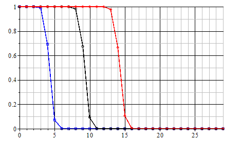
The figure below indicates the different steps of the eigenvalues decay rate for α=1/2\alpha=1/2 and different values of c . Each curve gives us an idea about the three areas of decay as well as these distributions in the interval (0.1).
Refer to caption
Figure 1: (a) Graph of λn(α)​(c)\lambda_{n}^{(\alpha)}(c)for α=0.5\alpha=0.5 and c=c=5π\pi (blue), c=10​πc=10\pi (black), c=15​πc=15\pi (red)

4 The eigenvalues distribution of finite Hankel transform

In this section, we concentrate on the distribution of λnα​(c)\lambda_{n}^{\alpha}(c) in the interval (0,1)(0,1) using the non-asymptotic behaviour of the trace and the Hilbert-Schmidt norm of the operator 𝒬cα.\mathcal{Q}_{c}^{\alpha}.

Theorem 3.

Let α>−1/2\alpha>-1/2 and c≥1c\geq 1, then we have

trace​(𝒬cα)=cπ−α2+γα​(c)c,\mbox{trace}(\mathcal{Q}_{c}^{\alpha})=\frac{c}{\pi}-\frac{\alpha}{2}+\frac{\gamma_{\alpha}(c)}{c}, (31)

where |γα​(c)|≤γα=γα1+α​γα2|\gamma_{\alpha}(c)|\leq\gamma_{\alpha}=\gamma^{1}_{\alpha}+\alpha\gamma^{2}_{\alpha} and

γα1\displaystyle\gamma^{1}_{\alpha} =\displaystyle= [(|μα|+2​α+1)2−(2​α+3)2+(2​α+1)​|μα|​|μα+1|4​π]\displaystyle\left[\displaystyle\frac{(|\mu_{\alpha}|+2\alpha+1)^{2}-(2\alpha+3)^{2}+(2\alpha+1)|\mu_{\alpha}||\mu_{\alpha+1}|}{4\pi}\right]
+\displaystyle+ 12​[hα+hα+1+(1+2π​(2​α+1))​(Cα​(1+|μα+1|2)+Cα+1​(1+|μα|2))]\displaystyle\frac{1}{2}\left[h_{\alpha}+h_{\alpha+1}+\left(1+\sqrt{\frac{2}{\pi}}(2\alpha+1)\right)\displaystyle\left(C_{\alpha}(1+\frac{|\mu_{\alpha+1}|}{2})+C_{\alpha+1}(1+\frac{|\mu_{\alpha}|}{2})\right)\right]

γα2=(1+|μα|)​(1+|μα+1|)π,\gamma^{2}_{\alpha}=\frac{\left(1+|\mu_{\alpha}|\right)\left(1+|\mu_{\alpha+1}|\right)}{\pi}, hα=Cα2+Cα​(1+|μα|2)h_{\alpha}=C_{\alpha}^{2}+C_{\alpha}(1+\frac{|\mu_{\alpha}|}{2}) , μα=α2−1/4\mu_{\alpha}=\alpha^{2}-1/4 and CαC_{\alpha} is given by (11).

Proof.

By the Mercer theorem, the trace of a kernel operator ℋ\mathcal{H} is of the form

trace​(ℋ)=∫IH⁡(x,x)​𝑑x.\mbox{trace}(\mathcal{H})=\int_{I}H(x,x)dx.

Then

trace​(𝒬cα)\displaystyle\mbox{trace}(\mathcal{Q}_{c}^{\alpha}) =\displaystyle= c​∫01Gα​(c​x,c​x)​𝑑x=∫0cGα​(x,x)​𝑑x\displaystyle c\int_{0}^{1}G_{\alpha}(cx,cx)dx=\int_{0}^{c}G_{\alpha}(x,x)dx
=\displaystyle= 12​∫0c(x​Jα+1​(x))′​Jα​(x)​𝑑x−12​∫0cx​Jα+1​(x)​Jα′​(x)​𝑑x\displaystyle\frac{1}{2}\int_{0}^{c}(xJ_{\alpha+1}(x))^{\prime}J_{\alpha}(x)dx-\frac{1}{2}\int_{0}^{c}xJ_{\alpha+1}(x)J_{\alpha}^{\prime}(x)dx
=\displaystyle= c2​Jα+1​(c)​Jα​(c)−∫0cx​Jα+1​(x)​Jα′​(x)​𝑑x.\displaystyle\frac{c}{2}J_{\alpha+1}(c)J_{\alpha}(c)-\int_{0}^{c}xJ_{\alpha+1}(x)J_{\alpha}^{\prime}(x)dx.

From [15], we have x​Jα′​(x)=−x​Jα+1​(x)+α​Jα​(x).xJ_{\alpha}^{\prime}(x)=-xJ_{\alpha+1}(x)+\alpha J_{\alpha}(x). Then we obtain

trace​(𝒬cα)=c2​Jα+1​(c)​Jα​(c)−α​∫0cJα+1​(x)​Jα​(x)​𝑑x+∫0cx​Jα+12​(x)​𝑑x.\mbox{trace}(\mathcal{Q}_{c}^{\alpha})=\frac{c}{2}J_{\alpha+1}(c)J_{\alpha}(c)-\alpha\int_{0}^{c}J_{\alpha+1}(x)J_{\alpha}(x)dx+\int_{0}^{c}xJ_{\alpha+1}^{2}(x)dx.

From [15] again, we have

∫0cx​Jα+12​(x)​𝑑x=c22​(Jα+12​(c)−Jα​(c)​Jα+2​(c))\int_{0}^{c}xJ_{\alpha+1}^{2}(x)dx=\frac{c^{2}}{2}\left(J_{\alpha+1}^{2}(c)-J_{\alpha}(c)J_{\alpha+2}(c)\right)

and

Jα+2​(c)=2​(α+1)c​Jα+1​(c)−Jα​(c).J_{\alpha+2}(c)=\frac{2(\alpha+1)}{c}J_{\alpha+1}(c)-J_{\alpha}(c).

One gets

trace​(𝒬cα)=c22​(Jα+12​(c)+Jα2​(c)−2​α+1c​Jα​(c)​Jα+1​(c))−α​∫0cJα+1​(x)​Jα​(x)​𝑑x.\mbox{trace}(\mathcal{Q}_{c}^{\alpha})=\frac{c^{2}}{2}\left(J_{\alpha+1}^{2}(c)+J_{\alpha}^{2}(c)-\frac{2\alpha+1}{c}J_{\alpha}(c)J_{\alpha+1}(c)\right)-\alpha\int_{0}^{c}J_{\alpha+1}(x)J_{\alpha}(x)dx.

Moreover, from [13], we have ∫0∞Jα+1​(x)​Jα​(x)​𝑑x=12.\int_{0}^{\infty}J_{\alpha+1}(x)J_{\alpha}(x)dx=\frac{1}{2}. Then we obtain

trace​(𝒬cα)=c22​(Jα+12​(c)+Jα2​(c)−2​α+1c​Jα​(c)​Jα+1​(c))−α2+α​∫c∞Jα+1​(x)​Jα​(x)​𝑑x.\mbox{trace}(\mathcal{Q}_{c}^{\alpha})=\frac{c^{2}}{2}\left(J_{\alpha+1}^{2}(c)+J_{\alpha}^{2}(c)-\frac{2\alpha+1}{c}J_{\alpha}(c)J_{\alpha+1}(c)\right)-\frac{\alpha}{2}+\alpha\int_{c}^{\infty}J_{\alpha+1}(x)J_{\alpha}(x)dx. (32)

By (11), we have

Jα​(x)=2π​x​rα​(x)+ηα​(x)x5/2,J_{\alpha}(x)=\sqrt{\frac{2}{\pi x}}r_{\alpha}(x)+\frac{\eta_{\alpha}(x)}{x^{5/2}}, (33)

where rα​(x)=(cos​(x−ωα)−(α2−1/4)​sin​(x−ωα)2​x)r_{\alpha}(x)=\left(\mbox{cos}(x-\omega_{\alpha})-(\alpha^{2}-1/4)\displaystyle\frac{\mbox{sin}(x-\omega_{\alpha})}{2x}\right) and supx≥0|ηα​(x)|≤Cα.\sup_{x\geq 0}|\eta_{\alpha}(x)|\leq C_{\alpha}.
A straightforward computation gives us

c22​(Jα+12​(c)+Jα2​(c)−2​α+1c​Jα​(c)​Jα+1​(c))=cπ​(rα+12​(c)+rα2​(c)−2​α+1c​rα​(c)​rα+1​(c))+hα(2)​(c)c,\frac{c^{2}}{2}\left(J_{\alpha+1}^{2}(c)+J_{\alpha}^{2}(c)-\frac{2\alpha+1}{c}J_{\alpha}(c)J_{\alpha+1}(c)\right)=\frac{c}{\pi}\left(r_{\alpha+1}^{2}(c)+r_{\alpha}^{2}(c)-\frac{2\alpha+1}{c}r_{\alpha}(c)r_{\alpha+1}(c)\right)+\frac{h_{\alpha}^{(2)}(c)}{c}, (34)

where

|hα(2)​(c)|≤12​[hα+hα+1+2π​(2​α+1)​(Cα​(1+|μα+1|2)+Cα+1​(1+|μα|2))].|h_{\alpha}^{(2)}(c)|\leq\frac{1}{2}\left[h_{\alpha}+h_{\alpha+1}+\sqrt{\frac{2}{\pi}}(2\alpha+1)\displaystyle\left(C_{\alpha}(1+\frac{|\mu_{\alpha+1}|}{2})+C_{\alpha+1}(1+\frac{|\mu_{\alpha}|}{2})\right)\right].

Here hα=Cα2+Cα​(1+|μα|2)h_{\alpha}=C_{\alpha}^{2}+C_{\alpha}(1+\frac{|\mu_{\alpha}|}{2}) and μα=α2−1/4.\mu_{\alpha}=\alpha^{2}-1/4.
On the other hand, we have

cπ​(rα+12​(c)+rα2​(c)−2​α+1c​rα​(c)​rα+1​(c))\displaystyle\frac{c}{\pi}\left(r_{\alpha+1}^{2}(c)+r_{\alpha}^{2}(c)-\frac{2\alpha+1}{c}r_{\alpha}(c)r_{\alpha+1}(c)\right) =\displaystyle= cπ+μα2+2​(2​α+1)​μα−4​(α+1)​cos2​(c−ωα)4​π​c\displaystyle\frac{c}{\pi}+\frac{\mu_{\alpha}^{2}+2(2\alpha+1)\mu_{\alpha}-4(\alpha+1)\mbox{cos}^{2}(c-\omega_{\alpha})}{4\pi c}
+\displaystyle+ (2​α+1)​μα​μα+1​sin​(2​c−2​ωα)4​π​c.\displaystyle\frac{(2\alpha+1)\mu_{\alpha}\mu_{\alpha+1}\mbox{sin}(2c-2\omega_{\alpha})}{4\pi c}.

We conclude from the last equality and (34) that

c22​(Jα+12​(c)+Jα2​(c)−2​α+1c​Jα​(c)​Jα+1​(c))=cπ+hα(1)​(c)+hα(2)​(c)c=cπ+γα(1)​(c)c,\frac{c^{2}}{2}\left(J_{\alpha+1}^{2}(c)+J_{\alpha}^{2}(c)-\frac{2\alpha+1}{c}J_{\alpha}(c)J_{\alpha+1}(c)\right)=\frac{c}{\pi}+\frac{h_{\alpha}^{(1)}(c)+h_{\alpha}^{(2)}(c)}{c}=\frac{c}{\pi}+\frac{\gamma_{\alpha}^{(1)}(c)}{c}, (35)

where |hα(1)​(c)|≤μα2+2​(2​α+1)​|μα|+4​(α+1)+(2​α+1)​|μα|​|μα+1|4​π.|h_{\alpha}^{(1)}(c)|\leq\displaystyle\frac{\mu_{\alpha}^{2}+2(2\alpha+1)|\mu_{\alpha}|+4(\alpha+1)+(2\alpha+1)|\mu_{\alpha}||\mu_{\alpha+1}|}{4\pi}.
Let’s proove now that ∫c∞Jα+1​(x)​Jα​(x)​𝑑x=γα(2)​(c)c\int_{c}^{\infty}J_{\alpha+1}(x)J_{\alpha}(x)dx=\frac{\gamma_{\alpha}^{(2)}(c)}{c} where γα(2)​(c)\gamma_{\alpha}^{(2)}(c) is bounded. By (33), we have

Jα+1​(x)​Jα​(x)=2π​x​rα+1​(x)​rα​(x)+2π​fα​(x)x3,J_{\alpha+1}(x)J_{\alpha}(x)=\frac{2}{\pi x}r_{\alpha+1}(x)r_{\alpha}(x)+\sqrt{\frac{2}{\pi}}\frac{f_{\alpha}(x)}{x^{3}}, (36)

where fα​(x)=rα​(x)​ηα+1​(x)+rα+1​(x)​ηα​(x)f_{\alpha}(x)=r_{\alpha}(x)\eta_{\alpha+1}(x)+r_{\alpha+1}(x)\eta_{\alpha}(x) that is |fα​(x)|≤Cα​(1+|μα+1|2)+Cα+1​(1+|μα|2).|f_{\alpha}(x)|\leq C_{\alpha}(1+\frac{|\mu_{\alpha+1}|}{2})+C_{\alpha+1}(1+\frac{|\mu_{\alpha}|}{2}). Note that

∫c∞Jα+1​(x)​Jα​(x)​𝑑x=2π​∫c∞rα+1​(x)​rα​(x)x​𝑑x+2π​∫c∞fα​(x)x3​𝑑x.\int_{c}^{\infty}J_{\alpha+1}(x)J_{\alpha}(x)dx=\frac{2}{\pi}\int_{c}^{\infty}\frac{r_{\alpha+1}(x)r_{\alpha}(x)}{x}dx+\sqrt{\frac{2}{\pi}}\int_{c}^{\infty}\frac{f_{\alpha}(x)}{x^{3}}dx. (37)

First, we have

|∫c∞fα​(x)x3​𝑑x|≤Cα​(1+|μα+1|2)+Cα+1​(1+|μα|2)2​c2=γα(2,0)c2.\left|\int_{c}^{\infty}\frac{f_{\alpha}(x)}{x^{3}}dx\right|\leq\frac{C_{\alpha}(1+\frac{|\mu_{\alpha+1}|}{2})+C_{\alpha+1}(1+\frac{|\mu_{\alpha}|}{2})}{2c^{2}}=\frac{\gamma_{\alpha}^{(2,0)}}{c^{2}}.

Second, a straightforward computation gives us

2​rα+1​(x)​rα​(x)x=sin​(2​x−2​ωα)x+μα+1​cos2​(x−ωα)−μα​sin2​(x−ωα)x2−μα​μα+1​sin​(2​x−2​ωα)4​x3.\frac{2r_{\alpha+1}(x)r_{\alpha}(x)}{x}=\frac{\mbox{sin}(2x-2\omega_{\alpha})}{x}+\frac{\mu_{\alpha+1}\mbox{cos}^{2}(x-\omega_{\alpha})-\mu_{\alpha}\mbox{sin}^{2}(x-\omega_{\alpha})}{x^{2}}-\mu_{\alpha}\mu_{\alpha+1}\frac{\mbox{sin}(2x-2\omega_{\alpha})}{4x^{3}}.
2π​∫c∞rα+1​(x)​rα​(x)x​𝑑x\displaystyle\frac{2}{\pi}\int_{c}^{\infty}\frac{r_{\alpha+1}(x)r_{\alpha}(x)}{x}dx =\displaystyle= ∫c∞sin​(2​x−2​ωα)π​x​𝑑x\displaystyle\int_{c}^{\infty}\frac{\mbox{sin}(2x-2\omega_{\alpha})}{\pi x}dx
+\displaystyle+ ∫c∞μα+1​cos2​(x−ωα)−μα​sin2​(x−ωα)π​x2​𝑑x\displaystyle\int_{c}^{\infty}\frac{\mu_{\alpha+1}\mbox{cos}^{2}(x-\omega_{\alpha})-\mu_{\alpha}\mbox{sin}^{2}(x-\omega_{\alpha})}{\pi x^{2}}dx
−\displaystyle- μα​μα+1​∫c∞sin​(2​x−2​ωα)4​π​x3.\displaystyle\mu_{\alpha}\mu_{\alpha+1}\int_{c}^{\infty}\frac{\mbox{sin}(2x-2\omega_{\alpha})}{4\pi x^{3}}.
|∫c∞sin​(2​x−2​ωα)π​x​𝑑x|=|cos​(2​x−2​ωα)2​π​c−∫c∞cos​(2​x−2​ωα)2​π​x2​𝑑x|≤12​π​c=γα(2,1)c.\left|\int_{c}^{\infty}\frac{\mbox{sin}(2x-2\omega_{\alpha})}{\pi x}dx\right|=\left|\frac{\mbox{cos}(2x-2\omega_{\alpha})}{2\pi c}-\int_{c}^{\infty}\frac{\mbox{cos}(2x-2\omega_{\alpha})}{2\pi x^{2}}dx\right|\leq\frac{1}{2\pi c}=\frac{\gamma_{\alpha}^{(2,1)}}{c}.
|∫c∞μα+1​cos2​(x−ωα)−μα​sin2​(x−ωα)π​x2​𝑑x|≤|μα+1|+|μα|π​c=γα(2,2)c.\left|\int_{c}^{\infty}\frac{\mu_{\alpha+1}\mbox{cos}^{2}(x-\omega_{\alpha})-\mu_{\alpha}\mbox{sin}^{2}(x-\omega_{\alpha})}{\pi x^{2}}dx\right|\leq\frac{|\mu_{\alpha+1}|+|\mu_{\alpha}|}{\pi c}=\frac{\gamma_{\alpha}^{(2,2)}}{c}.

and

|μα​μα+1​∫c∞sin​(2​x−2​ωα)4​π​x3​𝑑x|≤|μα+1|​|μα|8​π​c2=γα(2,3)c2\left|\mu_{\alpha}\mu_{\alpha+1}\int_{c}^{\infty}\frac{\mbox{sin}(2x-2\omega_{\alpha})}{4\pi x^{3}}dx\right|\leq\frac{|\mu_{\alpha+1}||\mu_{\alpha}|}{8\pi c^{2}}=\frac{\gamma_{\alpha}^{(2,3)}}{c^{2}}

Finally, we have

∫c∞Jα+1​(x)​Jα​(x)​𝑑x=γα(2)​(c)c,\int_{c}^{\infty}J_{\alpha+1}(x)J_{\alpha}(x)dx=\frac{\gamma_{\alpha}^{(2)}(c)}{c}, (38)

where |γα(2)​(c)|≤γα(2,0)+γα(2,1)+γα(2,2)+γα(2,3)=γα(2).|\gamma_{\alpha}^{(2)}(c)|\leq\gamma_{\alpha}^{(2,0)}+\gamma_{\alpha}^{(2,1)}+\gamma_{\alpha}^{(2,2)}+\gamma_{\alpha}^{(2,3)}=\gamma_{\alpha}^{(2)}. By (38), (32) and (35), we obtain

trace​(𝒬cα)=cπ−α2+γα(1)​(c)+α​γα(2)​(c)c.\mbox{trace}(\mathcal{Q}_{c}^{\alpha})=\frac{c}{\pi}-\frac{\alpha}{2}+\frac{\gamma_{\alpha}^{(1)}(c)+\alpha\gamma_{\alpha}^{(2)}(c)}{c}. (39)

∎

In the figure bellow, we illustrate the previous result of this work, which is given by Theorem 3. That is trace​(𝒬cα)−(cπ−α2)\mbox{trace}(\mathcal{Q}_{c}^{\alpha})-\left(\frac{c}{\pi}-\frac{\alpha}{2}\right) is comparable to 1/c1/c with different values of cc and α.\alpha.

Refer to caption
Figure 2: (a) Graph of trace​(𝒬cα)−(cπ−α2)\mbox{trace}(\mathcal{Q}_{c}^{\alpha})-(\frac{c}{\pi}-\frac{\alpha}{2}) (red) for α=5/2\alpha=5/2 (a), α=0.55\alpha=0.55 (b), α=1/2\alpha=1/2 (c) and graph of 1/c (blue)
Let​C\displaystyle\mbox{Let}\hskip 2.84526ptC =\displaystyle= 2π​[2​Cα+1​(O)​(1+π2​Cα​(O))+Cα​(K)​(3​α+72)​Cα+2​(O)+(α+32)​Cα​(O)2​(α+1)]\displaystyle\sqrt{\frac{2}{\pi}}\left[2C_{\alpha+1}(O)\left(1+\sqrt{\frac{\pi}{2}}C_{\alpha}(O)\right)+C_{\alpha}(K)\frac{(3\alpha+\frac{7}{2})C_{\alpha+2}(O)+(\alpha+\frac{3}{2})C_{\alpha}(O)}{2(\alpha+1)}\right] (40)
+\displaystyle+ 2π​[π2​Cα+1​(O)​((32+α)​Cα​(O)+Cα+1​(K))+Cα+1​(K)+(52+α)​Cα+1​(O)+Cα+2​(K)].\displaystyle\sqrt{\frac{2}{\pi}}\left[\sqrt{\frac{\pi}{2}}C_{\alpha+1}(O)\left((\frac{3}{2}+\alpha)C_{\alpha}(O)+C_{\alpha+1}(K)\right)+C_{\alpha+1}(K)+(\frac{5}{2}+\alpha)C_{\alpha+1}(O)+C_{\alpha+2}(K)\right].
Theorem 4.

Let α>−1/2\alpha>-1/2, c≥1c\geq 1 and (λnα​(c))(\lambda_{n}^{\alpha}(c)) be the sequence of eigenvalue of the integral operator 𝒬cα\mathcal{Q}_{c}^{\alpha}. For every 0<ϵ<1/20<\epsilon<1/2, we have

#{n;ϵ<λnα(c)<1−ϵ}≤16​[ln​(cπ)2​π2+34​π3+ln⁡(83)π2+2​cπ+1.123]+2​C2+4​κ1​ln​(2)+κ2c2ϵ⁡(1−ϵ),\#\{n;\epsilon<\lambda_{n}^{\alpha}(c)<1-\epsilon\}\leq\frac{16\left[\frac{\mbox{ln}(\frac{c}{\pi})}{2\pi^{2}}+\frac{3}{4\pi^{3}}+\frac{\ln(\frac{8}{3})}{\pi^{2}}+\frac{2c}{\pi}+1.123\right]+2C^{2}+4\kappa_{1}\mbox{ln}(2)+\frac{\kappa_{2}}{c^{2}}}{\epsilon(1-\epsilon)}, (41)

where κ1=4π2​(1+(1+π2​Cα​(O))2)\kappa_{1}=\frac{4}{\pi^{2}}\left(1+(1+\sqrt{\frac{\pi}{2}}C_{\alpha}(O))^{2}\right), κ2=8​Cα+12​(K)π2​(1+(1+π2​Cα​(O))2)\kappa_{2}=\frac{8C^{2}_{\alpha+1}(K)}{\pi^{2}}\left(1+(1+\sqrt{\frac{\pi}{2}}C_{\alpha}(O))^{2}\right) and Cα​(O),Cα​(K)C_{\alpha}(O),C_{\alpha}(K) have been given by (7) and (10).

Proof.

The Hilbert-Schmidt norm of 𝒬cα\mathcal{Q}_{c}^{\alpha} is given by

‖𝒬cα‖H​S\displaystyle||\mathcal{Q}_{c}^{\alpha}||_{HS} =\displaystyle= ∫01∫01(Kcα​(x,y))2​𝑑x​𝑑y\displaystyle\int_{0}^{1}\int_{0}^{1}\left(K_{c}^{\alpha}(x,y)\right)^{2}dxdy (42)
=\displaystyle= ∫01∫0∞(Kcα​(x,y))2​𝑑x​𝑑y−∫01∫1∞(Kcα​(x,y))2​𝑑x​𝑑y\displaystyle\int_{0}^{1}\int_{0}^{\infty}\left(K_{c}^{\alpha}(x,y)\right)^{2}dxdy-\int_{0}^{1}\int_{1}^{\infty}\left(K_{c}^{\alpha}(x,y)\right)^{2}dxdy (43)

The Palley-Wienner space

ℬcα={f∈L2​(0,∞);Support​ℋα​(f)⊂[0,c]}\mathcal{B}_{c}^{\alpha}=\{f\in L^{2}(0,\infty);\,\ \mbox{Support}\mathcal{H}^{\alpha}(f)\subset[0,c]\}

is a reproducing kernel Hilbert space,see [3]. Indeed, from the Hankel inversion theorem, for every f∈ℬcα,f\in\mathcal{B}_{c}^{\alpha}, we have

f⁡(x)=∫0cx​y​Jα​(x​y)​ℋα​(f)​(y)​𝑑y.f(x)=\int_{0}^{c}\sqrt{xy}J_{\alpha}(xy)\mathcal{H}^{\alpha}(f)(y)dy.

One gets by the Cauchy-Schwarz inequality and Parseval’s theorem that, for all x≥0x\geq 0

|f⁡(x)|≤c​Cα​(O)​‖ℋα​(f)‖L2​(0,∞)=c​Cα​(O)||f||L2​(0,∞).|f(x)|\leq\sqrt{c}\hskip 1.70717ptC_{\alpha}(O)||\mathcal{H}^{\alpha}(f)||_{L^{2}(0,\infty)}=\sqrt{c}\hskip 1.70717ptC_{\alpha}(O)||f||_{L^{2}(0,\infty)}.

It then follows that

Kcα​(x,x)=∫0∞(Kcα​(x,y))2​𝑑y.K_{c}^{\alpha}(x,x)=\int_{0}^{\infty}\left(K_{c}^{\alpha}(x,y)\right)^{2}dy. (44)

We conclude that

‖𝒬cα‖H​S\displaystyle||\mathcal{Q}_{c}^{\alpha}||_{HS} =\displaystyle= trace​(𝒬cα)−∫01∫1∞(Kcα​(x,y))2​𝑑y​𝑑x\displaystyle\mbox{trace}(\mathcal{Q}_{c}^{\alpha})-\int_{0}^{1}\int_{1}^{\infty}\left(K_{c}^{\alpha}(x,y)\right)^{2}dydx
=\displaystyle= trace​(𝒬cα)−∫0c∫c∞(Gα​(x,y))2​𝑑y​𝑑x\displaystyle\mbox{trace}(\mathcal{Q}_{c}^{\alpha})-\int_{0}^{c}\int_{c}^{\infty}\left(G_{\alpha}(x,y)\right)^{2}dydx
=\displaystyle= trace​(𝒬cα)−∫0c∫c2​c(Gα​(x,y))2​𝑑y​𝑑x−∫0c∫2​c∞(Gα​(x,y))2​𝑑y​𝑑x\displaystyle\mbox{trace}(\mathcal{Q}_{c}^{\alpha})-\int_{0}^{c}\int_{c}^{2c}\left(G_{\alpha}(x,y)\right)^{2}dydx-\int_{0}^{c}\int_{2c}^{\infty}\left(G_{\alpha}(x,y)\right)^{2}dydx
=\displaystyle= trace​(𝒬cα)−ℐ1​(c)−ℐ2​(c).\displaystyle\mbox{trace}(\mathcal{Q}_{c}^{\alpha})-\mathcal{I}_{1}(c)-\mathcal{I}_{2}(c).

One gets,

#{n;ϵ<λnα(c)<1−ϵ}\displaystyle\#\{n;\epsilon<\lambda_{n}^{\alpha}(c)<1-\epsilon\} ≤\displaystyle\leq ∑n=0∞λnα​(c)​(1−λnα​(c))ϵ⁡(1−ϵ)\displaystyle\frac{\displaystyle\sum_{n=0}^{\infty}\lambda_{n}^{\alpha}(c)(1-\lambda_{n}^{\alpha}(c))}{\epsilon(1-\epsilon)} (45)
=\displaystyle= trace​(𝒬cα)−‖𝒬cα‖H​Sϵ⁡(1−ϵ)=ℐ1​(c)+ℐ2​(c)ϵ⁡(1−ϵ).\displaystyle\frac{\mbox{trace}(\mathcal{Q}_{c}^{\alpha})-||\mathcal{Q}_{c}^{\alpha}||_{HS}}{\epsilon(1-\epsilon)}=\frac{\mathcal{I}_{1}(c)+\mathcal{I}_{2}(c)}{\epsilon(1-\epsilon)}. (46)

By (10), Jα​(x)=2π​x​(cos​(x−ωα)+ρα​(x)x)J_{\alpha}(x)=\sqrt{\frac{2}{\pi x}}\left(\mbox{cos}(x-\omega_{\alpha})+\frac{\rho_{\alpha}(x)}{x}\right) with supx≥0|ρα​(x)|≤π2​Cα​(K)\sup_{x\geq 0}\left|\rho_{\alpha}(x)\right|\leq\sqrt{\frac{\pi}{2}}C_{\alpha}(K).
Then the kernel GαG_{\alpha} has the following form

Gα​(x,y)\displaystyle G_{\alpha}(x,y) =\displaystyle= 2π​[x​sin​(x−ωα)​cos​(y−ωα)−y​sin​(y−ωα)​cos​(x−ωα)x2−y2]\displaystyle\frac{2}{\pi}\left[\frac{x\mbox{sin}(x-\omega_{\alpha})\mbox{cos}(y-\omega_{\alpha})-y\mbox{sin}(y-\omega_{\alpha})\mbox{cos}(x-\omega_{\alpha})}{x^{2}-y^{2}}\right] (47)
+\displaystyle+ 2π​[ρα​(y)y​x​sin​(x−ωα)−ρα​(x)x​y​sin​(y−ωα)x2−y2]\displaystyle\frac{2}{\pi}\left[\frac{\frac{\rho_{\alpha}(y)}{y}x\mbox{sin}(x-\omega_{\alpha})-\frac{\rho_{\alpha}(x)}{x}y\mbox{sin}(y-\omega_{\alpha})}{x^{2}-y^{2}}\right]
+\displaystyle+ 2π​[ρα+1​(x)​cos​(y−ωα)−ρα+1​(y)​cos​(x−ωα)x2−y2]\displaystyle\frac{2}{\pi}\left[\frac{\rho_{\alpha+1}(x)\mbox{cos}(y-\omega_{\alpha})-\rho_{\alpha+1}(y)\mbox{cos}(x-\omega_{\alpha})}{x^{2}-y^{2}}\right]
+\displaystyle+ 2π​[ρα+1​(x)​ρα​(y)y−ρα+1​(y)​ρα​(x)xx2−y2].\displaystyle\frac{2}{\pi}\left[\frac{\rho_{\alpha+1}(x)\frac{\rho_{\alpha}(y)}{y}-\rho_{\alpha+1}(y)\frac{\rho_{\alpha}(x)}{x}}{x^{2}-y^{2}}\right].

Using the inequality (∑k=1nak)2≤n​∑k=1n(ak)2,\left(\sum_{k=1}^{n}a_{k}\right)^{2}\leq n\sum_{k=1}^{n}(a_{k})^{2}, we obtain

ℐ2​(c)=∫0c∫2​c∞(Gα​(x,y))2​𝑑y​𝑑x\displaystyle\mathcal{I}_{2}(c)=\int_{0}^{c}\int_{2c}^{\infty}\left(G_{\alpha}(x,y)\right)^{2}dydx ≤\displaystyle\leq 4​κ1​∫0c∫2​c∞d​y​d​x(y−x)2+4​κ2​∫0c∫2​c∞d​y​d​x(y2−x2)2\displaystyle 4\kappa_{1}\int_{0}^{c}\int_{2c}^{\infty}\frac{dydx}{(y-x)^{2}}+4\kappa_{2}\int_{0}^{c}\int_{2c}^{\infty}\frac{dydx}{(y^{2}-x^{2})^{2}} (48)
≤\displaystyle\leq 4​κ1​ln​(2)+κ2c2,\displaystyle 4\kappa_{1}\mbox{ln}(2)+\frac{\kappa_{2}}{c^{2}}, (49)

with κ1=4π2​(1+(1+π2​Cα​(O))2)\kappa_{1}=\frac{4}{\pi^{2}}\left(1+(1+\sqrt{\frac{\pi}{2}}C_{\alpha}(O))^{2}\right) and κ2=8​Cα+12​(K)π2​(1+(1+π2​Cα​(O))2).\kappa_{2}=\frac{8C^{2}_{\alpha+1}(K)}{\pi^{2}}\left(1+(1+\sqrt{\frac{\pi}{2}}C_{\alpha}(O))^{2}\right).
For the last integral ℐ1​(c)\mathcal{I}_{1}(c), using (47) we have

Gα​(x,y)=Lα1​(x,y)+Lα2​(x,y),G_{\alpha}(x,y)=L^{1}_{\alpha}(x,y)+L^{2}_{\alpha}(x,y),

where

Lα1​(x,y)=2π​[x​sin​(x−ωα)​cos​(y−ωα)−y​sin​(y−ωα)​cos​(x−ωα)x2−y2]L^{1}_{\alpha}(x,y)=\frac{2}{\pi}\left[\frac{x\mbox{sin}(x-\omega_{\alpha})\mbox{cos}(y-\omega_{\alpha})-y\mbox{sin}(y-\omega_{\alpha})\mbox{cos}(x-\omega_{\alpha})}{x^{2}-y^{2}}\right]

and Lα2​(x,y)=γα​(x,y)cL^{2}_{\alpha}(x,y)=\frac{\gamma_{\alpha}(x,y)}{c}, where |γα​(x,y)|≤C|\gamma_{\alpha}(x,y)|\leq C and CC as given by (40).
Note that

ℐ1​(c)\displaystyle\mathcal{I}_{1}(c) =\displaystyle= ∫0c∫c2​c(Lα1​(x,y)+Lα2​(x,y))2​𝑑y​𝑑x\displaystyle\int_{0}^{c}\int_{c}^{2c}\left(L^{1}_{\alpha}(x,y)+L^{2}_{\alpha}(x,y)\right)^{2}dydx
≤\displaystyle\leq 2​c2​∫01∫12(Lα1​(c​x,c​y))2​𝑑y​𝑑x+2​C2\displaystyle 2c^{2}\int_{0}^{1}\int_{1}^{2}\left(L^{1}_{\alpha}(cx,cy)\right)^{2}dydx+2C^{2}
≤\displaystyle\leq 8π2​∫01∫12[c​x​sinc​(cπ​(x−y))x+y+sin​(c​y−ωα)​cos​(c​x−ωα)x+y]2​𝑑y​𝑑x+2​C2\displaystyle\frac{8}{\pi^{2}}\int_{0}^{1}\int_{1}^{2}\left[\frac{cx\mbox{sinc}(\frac{c}{\pi}(x-y))}{x+y}+\frac{\mbox{sin}(cy-\omega_{\alpha})\mbox{cos}(cx-\omega_{\alpha})}{x+y}\right]^{2}dydx+2C^{2}
≤\displaystyle\leq 16​c2π2​∫01∫12[sinc​(cπ​(x−y))]2​𝑑y​𝑑x+16​ln​(4/3)π2+2​C2.\displaystyle\frac{16c^{2}}{\pi^{2}}\int_{0}^{1}\int_{1}^{2}\left[\mbox{sinc}(\frac{c}{\pi}(x-y))\right]^{2}dydx+\frac{16\mbox{ln}(4/3)}{\pi^{2}}+2C^{2}.

Using the fact that [0,1]×[1,2]=D1∪D2∪D3∪D4,[0,1]\times[1,2]=D_{1}\cup D_{2}\cup D_{3}\cup D_{4}, where

D1={(x,y),1/2<x<1,−x+2<y<x+1}D_{1}=\{(x,y),\hskip 5.69054pt1/2<x<1,\hskip 5.69054pt-x+2<y<x+1\}
D2={(x,y),0<x<1/2,x+1<y<−x+2}D_{2}=\{(x,y),\hskip 5.69054pt0<x<1/2,\hskip 5.69054ptx+1<y<-x+2\}
D3={(x,y),0<x<1,y<x+1,y<−x+2}D_{3}=\{(x,y),\hskip 5.69054pt0<x<1,\hskip 5.69054pty<x+1,\hskip 5.69054pty<-x+2\}
D4={(x,y),0<x⁡<1,y>​x+1,y>−x+2}D_{4}=\{(x,y),\hskip 5.69054pt0<x<1,\hskip 5.69054pty>x+1,\hskip 5.69054pty>-x+2\}

and the following change of variables u=x−y,t=yu=x-y,t=y with the techniques of [6] , one gets

ℐ1​(c)≤16​[ln​(cπ)2​π2+34​π3+ln⁡(83)π2+2​cπ+1.123]+2​C2.\mathcal{I}_{1}(c)\leq 16\left[\frac{\mbox{ln}(\frac{c}{\pi})}{2\pi^{2}}+\frac{3}{4\pi^{3}}+\frac{\ln(\frac{8}{3})}{\pi^{2}}+\frac{2c}{\pi}+1.123\right]+2C^{2}. (50)

∎

5 Asymptotic Expansions for CPSWFs

In this section, we give a brief description of the computation and the decay rate of the series expansion coefficients of the eigenfunctions φn,cα\varphi_{n,c}^{\alpha} in a generalized Laguerre functions basis of L2​(0,∞)L^{2}(0,\infty) defined in (21), that is for all x≥0x\geq 0, we have

φn,cα​(x)=∑k=0∞βkn​(c)​ψk,αa​(x)\varphi_{n,c}^{\alpha}(x)=\sum_{k=0}^{\infty}\beta^{n}_{k}(c)\psi_{k,\alpha}^{a}(x) (51)

where βkn​(c)=∫0∞φn,cα​(x)​ψk,αa​(x)​𝑑x.\beta^{n}_{k}(c)=\int_{0}^{\infty}\varphi_{n,c}^{\alpha}(x)\psi_{k,\alpha}^{a}(x)dx.

Lemma 2.

Let a>0a>0 and 𝒟cα\mathcal{D}_{c}^{\alpha} be the Sturm-Liouville differential operator defined in (3). Then for every n≥0n\geq 0, we have

𝒟cα​(ψn,αa)=dnn−2​(a)​ψn−2,αa+dnn−1​(a)​ψn−1,αa+dnn​(a)​ψn,αa+dnn+1​(a)​ψn+1,αa+dnn+2​(a)​ψn+2,αa,\mathcal{D}_{c}^{\alpha}(\psi_{n,\alpha}^{a})=d_{n}^{n-2}(a)\psi_{n-2,\alpha}^{a}+d_{n}^{n-1}(a)\psi_{n-1,\alpha}^{a}+d_{n}^{n}(a)\psi_{n,\alpha}^{a}+d_{n}^{n+1}(a)\psi_{n+1,\alpha}^{a}+d_{n}^{n+2}(a)\psi_{n+2,\alpha}^{a}, (52)

where

dnn−2​(a)=(n−1)​n​(n+α−1)​(n+α)d_{n}^{n-2}(a)=\sqrt{(n-1)n(n+\alpha-1)(n+\alpha)}
dnn−1​(a)=−n⁡(n+α)​(c2a2−a2+4​(2​n+α+1))d_{n}^{n-1}(a)=-\sqrt{n(n+\alpha)}\left(\frac{c^{2}}{a^{2}}-a^{2}+4(2n+\alpha+1)\right)
dnn​(a)=α2−54+(2​n+α+1)​(c2a2+a2+3​(2​n+α)+2)d_{n}^{n}(a)=\alpha^{2}-\frac{5}{4}+(2n+\alpha+1)\left(\frac{c^{2}}{a^{2}}+a^{2}+3(2n+\alpha)+2\right)
dnn+1​(a)=−(n+1)​(n+α+1)​(c2a2−a2+4​(2​n+α+1))d_{n}^{n+1}(a)=-\sqrt{(n+1)(n+\alpha+1)}\left(\frac{c^{2}}{a^{2}}-a^{2}+4(2n+\alpha+1)\right)
dnn+2​(a)=(n+1)​(n+2)​(n+α+1)​(n+α+2)d_{n}^{n+2}(a)=\sqrt{(n+1)(n+2)(n+\alpha+1)(n+\alpha+2)}
Proof.

First, we have

dd​x​ψn,αa​(x)=(α+1/2x−a2​x)​ψn,αa​(x)+2​2​aα+3​xα+3/2​e−a2​x22​dd​x​(L~nα)​(a2​x2),\dfrac{d}{dx}\psi_{n,\alpha}^{a}(x)=(\frac{\alpha+1/2}{x}-a^{2}x)\psi_{n,\alpha}^{a}(x)+2\sqrt{2}a^{\alpha+3}x^{\alpha+3/2}e^{-\frac{a^{2}x^{2}}{2}}\dfrac{d}{dx}\left(\widetilde{L}_{n}^{\alpha}\right)(a^{2}x^{2}),

then

d2d​x2​ψn,αa​(x)\displaystyle\dfrac{d^{2}}{dx^{2}}\psi_{n,\alpha}^{a}(x) =\displaystyle= [α2−1/4x2−2​a2​(α+1/2)+a4​x2−a2]​ψn,αa​(x)\displaystyle\left[\frac{\alpha^{2}-1/4}{x^{2}}-2a^{2}(\alpha+1/2)+a^{4}x^{2}-a^{2}\right]\psi_{n,\alpha}^{a}(x)
+\displaystyle+ 4​2​aα+3​xα+1/2​e−a2​x22​[a2​x2​d2​L~nαd​x2​(a2​x2)+(α+1−a2​x2)​d​L~nαd​x​(a2​x2)].\displaystyle 4\sqrt{2}a^{\alpha+3}x^{\alpha+1/2}e^{-\frac{a^{2}x^{2}}{2}}\left[a^{2}x^{2}\frac{d^{2}\widetilde{L}_{n}^{\alpha}}{dx^{2}}(a^{2}x^{2})+(\alpha+1-a^{2}x^{2})\frac{d\widetilde{L}_{n}^{\alpha}}{dx}(a^{2}x^{2})\right].

By (17), we obtain

d2d​x2​ψn,αa​(x)=[α2−1/4x2−2​a2​(2​n+α+1)+a4​x2]​ψn,αa​(x).\dfrac{d^{2}}{dx^{2}}\psi_{n,\alpha}^{a}(x)=\left[\frac{\alpha^{2}-1/4}{x^{2}}-2a^{2}(2n+\alpha+1)+a^{4}x^{2}\right]\psi_{n,\alpha}^{a}(x).

Finally, one gets

𝒟cα​(ψn,αa)​(x)\displaystyle\mathcal{D}_{c}^{\alpha}(\psi_{n,\alpha}^{a})(x) =\displaystyle= 𝒟cα​(ψn,αa)=−dd​x​[(1−x2)​dd​x​ψn,αa​(x)]−(14−α2x2−c2​x2)​ψn,αa​(x)\displaystyle\mathcal{D}_{c}^{\alpha}(\psi_{n,\alpha}^{a})=-\dfrac{d}{dx}\left[(1-x^{2})\dfrac{d}{dx}\psi_{n,\alpha}^{a}(x)\right]-\left(\dfrac{\dfrac{1}{4}-\alpha^{2}}{x^{2}}-c^{2}x^{2}\right)\psi_{n,\alpha}^{a}(x) (53)
=\displaystyle= [(c2−a4)​x2+(α+1)2−1/4+2​a2​(2​n+α+1)+2​a2​x2​(2​n+α)+a4​x4]​ψn,αa​(x)\displaystyle\left[(c^{2}-a^{4})x^{2}+(\alpha+1)^{2}-1/4+2a^{2}(2n+\alpha+1)+2a^{2}x^{2}(2n+\alpha)+a^{4}x^{4}\right]\psi_{n,\alpha}^{a}(x)
+\displaystyle+ 4​2​aα+3​xα+5/2​e−a2​x22​d​L~nαd​x​(a2​x2).\displaystyle 4\sqrt{2}a^{\alpha+3}x^{\alpha+5/2}e^{-\frac{a^{2}x^{2}}{2}}\frac{d\widetilde{L}_{n}^{\alpha}}{dx}(a^{2}x^{2}).

By [13] and using (18), we have

a2​x2​d​L~nαd​x​(a2​x2)=(a2​x2−(n+α+1))​L~nα​(a2​x2)+((n+1)​(n+α+1))1/2​L~n+1α​(a2​x2),a^{2}x^{2}\frac{d\widetilde{L}_{n}^{\alpha}}{dx}(a^{2}x^{2})=(a^{2}x^{2}-(n+\alpha+1))\widetilde{L}_{n}^{\alpha}(a^{2}x^{2})+\left((n+1)(n+\alpha+1)\right)^{1/2}\widetilde{L}_{n+1}^{\alpha}(a^{2}x^{2}),
a2​x2​ψn,αa​(x)=−(n⁡(n+α))1/2​ψn−1,αa​(x)+(2​n+α+1)​ψn,αa​(x)−((n+1)​(n+α+1))1/2​ψn+1,αa​(x).a^{2}x^{2}\psi_{n,\alpha}^{a}(x)=-\left(n(n+\alpha)\right)^{1/2}\psi_{n-1,\alpha}^{a}(x)+(2n+\alpha+1)\psi_{n,\alpha}^{a}(x)-\left((n+1)(n+\alpha+1)\right)^{1/2}\psi_{n+1,\alpha}^{a}(x).

By using the two last equalities and (53), one gets the desired result. ∎

Proposition 2.

Let (χn,α​(c))\big(\chi_{n,\alpha}(c)\big) be the sequence of eigenvalues of the differential operator 𝒟cα\mathcal{D}_{c}^{\alpha}, then the sequence of coefficients (βkn​(c))\big(\beta_{k}^{n}(c)\big) satisfy the following recurssion formula, for every n≥0n\geq 0 and k≥0k\geq 0, we have

dk+2k​(a)​βk+2n​(c)+dk+1k​(a)​βk+1n​(c)+(dkk​(a)−χn,α​(c))​βkn​(c)+dk−1k​(a)​βk−1n​(c)+dk−2k​(a)​βk−2n​(c)=0,\displaystyle d_{k+2}^{k}(a)\beta_{k+2}^{n}(c)+d_{k+1}^{k}(a)\beta_{k+1}^{n}(c)+(d_{k}^{k}(a)-\chi_{n,\alpha}(c))\beta_{k}^{n}(c)+d_{k-1}^{k}(a)\beta_{k-1}^{n}(c)+d_{k-2}^{k}(a)\beta_{k-2}^{n}(c)=0, (54)

with d−11​(a)=d−20​(a)=d−10​(a)=0.d_{-1}^{1}(a)=d_{-2}^{0}(a)=d_{-1}^{0}(a)=0.

Remark 1.

The previous system can be written by the following eigensystem

M​D=χn,α​(c)​D,M=[mk,j]k,j≥0,D=[βkn​(c)]k≥0T,MD=\chi_{n,\alpha}(c)D,M=[m_{k,j}]_{k,j\geq 0},D=[\beta_{k}^{n}(c)]^{T}_{k\geq 0},

with mk,j=0,m_{k,j}=0, if |k−j|>2|k-j|>2 and mk,k=dkk​(a)m_{k,k}=d_{k}^{k}(a), mk,k−1=dk−1k​(a)m_{k,k-1}=d_{k-1}^{k}(a), mk,k−2=dk−2k​(a),m_{k,k-2}=d_{k-2}^{k}(a),
mk,k+1=dk+1k​(a)m_{k,k+1}=d_{k+1}^{k}(a) ,mk,k+2=dk+2k​(a).m_{k,k+2}=d_{k+2}^{k}(a). Moreover, for a=c,a=\sqrt{c}, the previous matrix becomes diagonally dominant when n<12​(c4−(α+1))n<\frac{1}{2}(\frac{c}{4}-(\alpha+1)) where we can use the Inverse Power Method for the computation of CPSWFs when c is large compared to the prolate’s order.

Proposition 3.

Let c>0c>0 be a positive real number, then there exists a constant δ0\delta_{0} and a positive integer k0k_{0} such that for any integer n≥max⁡(c2,cπ+k0)n\geq\max{(\frac{c}{2},\frac{c}{\pi}+k_{0})}, χn,α​(c)>max⁡(2​α2−1/2,c2​(4​α2−1))\chi_{n,\alpha}(c)>\max{(2\alpha^{2}-1/2,c^{2}(4\alpha^{2}-1))} and k≥nk\geq n , we have

|βkn​(c)|≤12​e​δ0​Mα​(k)(α+1)​(ca)α+1​e−(k+α+1/2)​ln⁡(k+α+1/22)+A2​(2​n+α+1)​ln⁡(πc​(n+k0)).|\beta^{n}_{k}(c)|\leq\frac{1}{\sqrt{2e\delta_{0}}}\dfrac{M_{\alpha}(k)}{(\alpha+1)}(\frac{c}{a})^{\alpha+1}e^{-(k+\alpha+1/2)\ln(\frac{k+\alpha+1/2}{2})+\frac{A}{2}(2n+\alpha+1)\ln(\frac{\pi}{c}(n+k_{0}))}. (55)

Where Mα​(k)={(α+1)kk!if ​α≥0(2−(α+1)kk!)if −1≤α≤0M_{\alpha}(k)=\begin{cases}\frac{(\alpha+1)_{k}}{k!}&\mbox{if }\alpha\geq 0\\ (2-\frac{(\alpha+1)_{k}}{k!})&\mbox{if }-1\leq\alpha\leq 0\end{cases}.

Proof.

First, from the Parseval’s equality, (5) and (21), we have

βkn​(c)\displaystyle\beta^{n}_{k}(c) =\displaystyle= ⟨φn,cα,ψk,αa⟩L2​(0,∞)=⟨ℋα​(φn,cα),ℋα​(ψk,αa)⟩L2​(0,∞)\displaystyle\left<\varphi_{n,c}^{\alpha},\psi_{k,\alpha}^{a}\right>_{L^{2}(0,\infty)}=\left<\mathcal{H}^{\alpha}(\varphi_{n,c}^{\alpha}),\mathcal{H}^{\alpha}(\psi_{k,\alpha}^{a})\right>_{L^{2}(0,\infty)}
=\displaystyle= (−1)ka​c​μn,α​(c)​⟨φn,cα​(.c)​χ[0,c],ψk,αa​(.a2)⟩L2​(0,∞)\displaystyle\frac{(-1)^{k}}{ac\mu_{n,\alpha}(c)}\left<\varphi_{n,c}^{\alpha}(\frac{.}{c})\chi_{[0,c]},\psi_{k,\alpha}^{a}(\frac{.}{a^{2}})\right>_{L^{2}(0,\infty)}
=\displaystyle= (−1)ka​μn,α​(c)⟨φn,cα,ψk,αa(ca2.)⟩L2​(0,1)\displaystyle\frac{(-1)^{k}}{a\mu_{n,\alpha}(c)}\left<\varphi_{n,c}^{\alpha},\psi_{k,\alpha}^{a}(\frac{c}{a^{2}}.)\right>_{L^{2}(0,1)}

Then, by the Cauchy-Schwarz inequality, one gets

|βkn(c)|≤1a​|μn,α​(c)|||ψk,αa(ca2.)||L2​(0,1).\displaystyle|\beta^{n}_{k}(c)|\leq\frac{1}{a|\mu_{n,\alpha}(c)|}||\psi_{k,\alpha}^{a}(\frac{c}{a^{2}}.)||_{L^{2}(0,1)}.

By [10], we have

||ψk,αa(ca2.)||L2​(0,1)≤cα+1/2​Mα​(k)aα​(α+1)​Γ​(k+α+1),||\psi_{k,\alpha}^{a}(\frac{c}{a^{2}}.)||_{L^{2}(0,1)}\leq\dfrac{c^{\alpha+1/2}M_{\alpha}(k)}{a^{\alpha}(\alpha+1)\Gamma(k+\alpha+1)},

where Mα​(k)={(α+1)kk!if ​α≥0(2−(α+1)kk!)if −1≤α≤0M_{\alpha}(k)=\begin{cases}\frac{(\alpha+1)_{k}}{k!}&\mbox{if }\alpha\geq 0\\ (2-\frac{(\alpha+1)_{k}}{k!})&\mbox{if }-1\leq\alpha\leq 0\end{cases}. Finally, from [4], [7] and the last inequality, one gets

|βkn​(c)|\displaystyle|\beta^{n}_{k}(c)| ≤\displaystyle\leq cα+1/2​Mα​(k)aα+1​(α+1)​Γ​(k+α+1)​1|μn,α​(c)|\displaystyle\dfrac{c^{\alpha+1/2}M_{\alpha}(k)}{a^{\alpha+1}(\alpha+1)\Gamma(k+\alpha+1)}\frac{1}{|\mu_{n,\alpha}(c)|}
≤\displaystyle\leq cα+1/2​Mα​(k)2​e​aα+1​(α+1)​(ek+α+1/2)k+α+1/2​cδ0​eA2​(2​n+α+1)​ln⁡(πc​(n+k0))\displaystyle\dfrac{c^{\alpha+1/2}M_{\alpha}(k)}{\sqrt{2e}a^{\alpha+1}(\alpha+1)}\left(\frac{e}{k+\alpha+1/2}\right)^{k+\alpha+1/2}\sqrt{\frac{c}{\delta_{0}}}e^{\frac{A}{2}(2n+\alpha+1)\ln(\frac{\pi}{c}(n+k_{0}))}
≤\displaystyle\leq cα+1​Mα​(k)2​e​δ0​aα+1​(α+1)​e−(k+α+1/2)​ln⁡(k+α+1/22)+A2​(2​n+α+1)​ln⁡(πc​(n+k0)).\displaystyle\dfrac{c^{\alpha+1}M_{\alpha}(k)}{\sqrt{2e\delta_{0}}a^{\alpha+1}(\alpha+1)}e^{-(k+\alpha+1/2)\ln(\frac{k+\alpha+1/2}{2})+\frac{A}{2}(2n+\alpha+1)\ln(\frac{\pi}{c}(n+k_{0}))}.

∎

References

  • [1] L. D. Abreu and A. S. Bandeira, Landau’s necessary conditions for the Hankel transform, J. Funct. Anal. 262(4), (2012), 1845–1866.
  • [2] G. E. Andrews, R. Askey and R. Roy, Special Functions, Cambridge University Press , Cambridge, New York, 1999.
  • [3] N.Aronszajn, Theory of reproducing Kernels, American Mathematical Society, Vol. 68, No. 3 (May, 1950), pp. 337-404.
  • [4] N. Batir, Inequalities for the gamma function, Arch. Math. 2008; 91(6): 554–56
  • [5] A. Bonami, P. Jaming and A. Karoui, Non-Asymptotic Behaviour of the Sinc-Kernel Operator and Related Applications, available at arXiv:1804.01257, (2018).
  • [6] A. Bonami and A. Karoui, Random Discretization of the Finite Fourier Transform and Related Kernel Random Matrices, available at arXiv:1703.10459, (2019).
  • [7] M. Boulsane and A. Karoui, The Finite Hankel Transform Operator: Some Explicit and Local Estimates of the Eigenfunctions and Eigenvalues Decay Rates, J. Four. Anal. Appl, Volume 24, Issue 6, pp 1554–1578, (2018).
  • [8] L. Gatteschi, Asymptotics and bounds for the zeros of Laguerre polynomials: a survey. Journal of Computational and Applied Mathematics, 144(1): 7-27, (2002).
  • [9] I. Krasikov, Approximation for the Bessel and airy functions with an explicit error term, LMS Journal of Computation and Mathematics, Volume 17, Issue 1 pp. 209-225, (2014).
  • [10] M.Michalska and J.Szynal, A new bound for the Laguerre polynomials, Journal of Computational and Applied Mathematics 133(1-2):489–493, (2001).
  • [11] D.Slepian, Prolate spheroidal wave functions, Fourier analysis and uncertainty–IV: Extensions to many dimensions; generalized prolate spheroidal functions, Bell System Tech. J. 43 (1964), 3009–3057.
  • [12] A.YA. Olenko, Upper bound on x​Jμ​(x)\sqrt{x}J_{\mu}(x) and its applications, Integral Transforms and Special Functions.Vol. 17, No. 6, June 2006, 455–467
  • [13] F.W.J. Olver, D.W. Lozier, R.F.Boisvert and C.W.Clark, NIST Handbook of Mathematical Functions, Cambridge University Press; New York; (2010).
  • [14] H. Xiao and V. Rokhlin, High-Frequency Asymptotic Expansions for Certain Prolate Spheroidal Wave Functions, J.Four. Anal. Appl.Volume 9, Issue 6, (2003).
  • [15] G. N. Watson, A treatise on the theory of Bessel functions.second edition, Cambridge University Press.(1966).