Deep synthesis regularization of inverse problems

Inverse problems are typically ill-posed. This means that even in the noise free case the solution of (1) is not unique or is unstable with respect to data perturbations. In order to overcome the ill-posedness, regularization methods have to be applied which incorporate suitable prior information that acts as a selection criterium and at the same time stabilizes the reconstruction [1, 2].

One of the most established stable reconstruction approaches is convex variational regularization. In this case one considers minimizers of the generalized Tikhonov functional

where $\mathcal{R}_{\mathbb{U}}\colon\mathbb{U}\rightarrow[0,\infty]$ is a convex regularizer on the signal space $\mathbb{U}$ and $\alpha>0$ is the regularization parameter. Several choices for the regularizer have been proposed and analysed. For example, the choice $\mathcal{R}_{\mathbb{U}}(u)=\lVert u\rVert_{\mathbb{U}}^{2}$ leads to quadratic Tikhonov regularization, choosing the regularizer as the total variation (TV) semi-norm $\mathcal{R}_{\mathbb{U}}(u)=\lVert\nabla u\rVert_{1}$ yields to TV-regularization, and choosing the $\ell^{1}$-norm $\mathcal{R}_{\mathbb{U}}(u)=\sum_{i\in\mathds{N}}\lvert\langle e_{i},u\rangle\rvert$ with respect to a given orthonormal basis $(e_{i})_{i\in\mathds{N}}$ yields to sparse $\ell^{1}$-regularization.

Convex variational regularization is build on a solid theoretical fundament. In particular, if $\mathcal{R}_{\mathbb{U}}$ is convex, lower semi-continuous and coercive on $\ker(\mathbf{K})^{\bot}$, then (2) is well-posed, stable and convergent as $\alpha\to 0$. Moreover, for elements $u\in\mathbb{U}$ satisfying the so-called source condition $\ran(\mathbf{K}^{*})\cap\partial\mathcal{R}_{\mathbb{U}}(u)\neq\emptyset$, convergence rates in the form of quantitative estimates between $u$ and solutions of (2) have been derived [1, 3].

Variational regularization (2) is based on the assumption that a small value of the regularizer is a good prior for the underlying signal-class. However, it is often challenging to hand-craft an appropriate regularization term for a given class of images. Frame-based methods address this issue by adjusting frames to the signal class and using a small value of the regularizer of the frame coefficients as image prior.

Let $(\varphi_{\lambda})_{\lambda\in\Lambda}$ be a frame of $\mathbb{U}$ and denote by $\boldsymbol{\Phi}\colon\ell^{2}(\Lambda)\to\mathbb{U}$ the synthesis operator that maps $\xi\in\ell^{2}(\Lambda)$ to the synthesized signal $\boldsymbol{\Phi}(\xi)\coloneqq\sum_{\lambda\in\Lambda}\xi_{\lambda}\varphi_{\lambda}$. Its adjoint $\boldsymbol{\Phi}^{*}$ is the analysis operator and maps $u\in\mathbb{U}$ to the so-called analysis coefficients $\boldsymbol{\Phi}^{*}(u)=(\langle\varphi_{\lambda},u\rangle)_{\lambda\in\Lambda}$. Two established frame based approaches are the following frame synthesis and frame analysis regularization, respectively,

Here $\mathcal{R}\colon\ell^{2}(\Lambda)\rightarrow[0,\infty]$ is a convex regularizer on the coefficient space and $\alpha>0$ the regularization parameter. Typical instances of frame analysis and frame synthesis regularization are when the regularizer $\mathcal{R}=\lVert\,\cdot\,\rVert_{1,\mathbf{w}}$ is taken as the (weighted) $\ell^{1}$-norm given by

where $w_{\lambda}>0$. In this case (4) enforces sparsity of the analysis coefficients $\boldsymbol{\Phi}^{*}(u)$, whereas (3) enforces sparsity of the synthesis coefficients of the signal. In the case of bases, the two approaches (3) and (4) are equivalent (if one of them is applied with the dual basis). In the redundant case, however, they are fundamentally different [4, 5].

Many different frame-based approaches for solving inverse problems have been analyzed [6, 7, 8, 4, 5]. However, these methods rely on linear synthesis operators which may not be appropriate for a given signal-class. Recently, non-linear deep learning and neural network based approaches showed outstanding performance for various imaging applications. Inspired by such methods, in this paper, we generalize the frame based synthesis approach to allow neural networks as synthesis operators. Because these representations are non-linear, the resulting approach requires new mathematical theory that we develop in this paper.

In this paper, we propose deep synthesis regularization (DESYRE) where we consider minimizers of

Here, $\mathbf{D}_{\alpha}\colon\ell^{2}(\Lambda)\rightarrow\mathbb{U}$ are possibly non-linear synthesis mappings and $\lVert\,\cdot\,\rVert_{1,\mathbf{w}}\colon\ell^{2}(\Lambda)\rightarrow[0,\infty]$ is the weighted $\ell^{1}$-norm defined by (5). The main theoretical results of this paper provide a complete convergence analysis for the DESYRE approach. The corresponding proofs closely follow [9, 1]. We point out, however, that the convergence results in these references cannot be directly applied to our setting because we allow the coefficient operators $\mathbf{K}\circ\mathbf{D}_{\alpha}$ in (6) to depend on $\alpha$. Using non-stationary synthesis mappings $\mathbf{D}_{\alpha}$ allows accounting for discretization as well as for approximate network training. In the recent years various deep learning based reconstruction methods have been derived which outperform classical variational regularization [10, 11, 12, 13]. However, rigorously analyzing them as regularization methods is challenging. DESYRE follows the deep learning strategy and, as we demonstrate in this paper, allows the derivation of results similar to classical sparse regularization.

In [14], a somehow dual approach to (6) has been studied, where minimizers of the NETT functional $\lVert\mathbf{K}u-v_{\delta}\rVert^{2}+\alpha\mathcal{R}(\mathbf{E}(u))$ have been considered, where $\mathbf{E}\colon\mathbb{U}\rightarrow\ell^{2}(\Lambda)$ is a non-linear analysis operator and $\mathcal{R}{}$ a regularizer. Due to the non-linearity of $\mathbf{E}$, the penalty $\mathcal{R}\circ\mathbf{E}$ is typically non-convex. One advantage of the deep synthesis method over the analysis counterpart is that the penalty term is still convex, which is beneficial for the theoretical analysis as well as the numerical minimization. Another strength of DESYRE is that the network can be trained without explicit knowledge of the operator $\mathbf{K}$. Thus, the proposed approach has some kind of universality like [15, 14, 16, 17, 18] in the sense that the network is trained independent of the specific forward operator and can be used for different inverse problems without retraining.

The rest of the paper is organized as follows. Section 2 gives a theoretical analysis of the proposed method. In Section 3 we propose a learned synthesis mapping. We present numerical results and compare DESYRE to other reconstruction methods in Section 4. The paper ends with a summary and outlook presented in Section 5. This paper is a significantly changed and extended version of the proceedings [19] presented at the SampTA 2019 in Bordeaux. The analysis of the proposed method and all the numerical results are completely new.

Throughout this paper we assume that the following assumption holds. For the following let $\mathbf{D},\mathbf{D}_{\alpha}\colon\ell^{2}(\Lambda)\to\mathbb{U}$ for $\alpha>0$ be given.

Assumption (R5) implies that $\lVert\,\cdot\,\rVert_{1,\mathbf{w}}$ is coercive. To see this, let $\xi\in\ell^{2}(\Lambda)$ and assume $\lVert\xi\rVert_{1,\mathbf{w}}<\infty$. Then, for all $\lambda\in\Lambda$, we have $w_{\lambda}\lvert\xi_{\lambda}\rvert/\lVert\xi\rVert_{1,\mathbf{w}}\leq 1$ and hence

This yields the estimate $\lVert\xi\rVert_{2}\leq\lVert\xi\rVert_{1,\mathbf{w}}/\underline{w}$ and proves the coercivity of $\lVert\,\cdot\,\rVert_{1,\mathbf{w}}$. Since the data-discrepancy term is non-negative this also shows the coercivity of the synthesis functional $\mathcal{S}_{\alpha,v_{\delta}}$ for every $\alpha>0$.

As the sum of non-negative convex and weakly continuous functionals, $\lVert\,\cdot\,\rVert_{1,\mathbf{w}}$ is convex and weakly lower semi-continuous. Assumptions (R2), (R4) imply that $(\mathbf{K}\circ\mathbf{D}_{\alpha})$ is weakly sequentially continuous. Moreover, the norm $\lVert\,\cdot\,\rVert_{\mathbb{V}}$ is weakly sequentially lower semi-continuous. This shows that $\mathcal{S}_{\alpha,v_{\delta}}$ is weakly lower semi-continuous as a sum of weakly lower semi-continuous functionals. Coercivity and weak lower semi-continuity basically yield the following well-posedness results for deep synthesis regularization.

An element in the set $\argmin\{\lVert\xi\rVert_{1,\mathbf{w}}\mid(\mathbf{K}\circ\mathbf{D})(\xi)=v\}$ is called $\lVert\,\cdot\,\rVert_{1,\mathbf{w}}$-minimizing solution of (7). Note that $\lVert\,\cdot\,\rVert_{1,\mathbf{w}}$-minimizing solutions exists whenever there is any solution $\xi$ with $\lVert\xi\rVert_{1,\mathbf{w}}<\infty$, see [1, Theorem 3.25]. For the following convergence results we make the following additional assumption

1. (R6)

   $\forall\rho>0\colon\Delta_{\rho}(\alpha)\coloneqq\sup_{\lVert\xi\rVert\leq\rho}\lVert\mathbf{D}_{\alpha}(\xi)-\mathbf{D}(\xi)\rVert\to 0$.

This assumption guarantees that $\mathbf{D}_{\alpha}$ arbitrarily well approximates $\mathbf{D}$ as $\alpha\to 0$.

The existence of a solution $\xi^{\dagger}$ to (7) always implies the existence of a solution $u^{\dagger}\coloneqq\mathbf{D}(\xi^{\dagger})$ to the original problem. Moreover, Theorem 2.4 shows strong convergence of the regularized solutions in the coefficient space $\ell^{2}(\Lambda)$. By assuming that the synthesis mappings $\mathbf{D}_{\alpha}$ are uniformly Lipschitz continuous we further get the strong convergence of the regularized solutions in the signal space.

A network is typically given as a composition of trained Lipschitz-continuous functions and given activation functions. The standard activation functions all satisfy a Lipschitz-continuity condition, e.g. the ReLU, $\tanh$ or sigmoid function are all Lipschitz-continuous. The uniform Lipschitz-continuity assumption on the networks $\mathbf{D}_{\alpha}$ can therefore easily be fulfilled.

Convergence rates name quantitative error estimates between exact and regularized solutions. In order to derive such results we have to make some additional assumptions on the interplay between the regularization functional and the operators $\mathbf{K}$, $\mathbf{D}$, $\mathbf{D}_{\alpha}$.

In the following we write $\alpha\asymp\delta$ if $C_{1}\delta\leq\alpha(\delta)\leq C_{2}\delta$ for $\delta>0$ and some constants $C_{1},C_{2}>0$.

Following the deep learning paradigm we select the synthesis operator $\mathbf{D}$ from a parametrized class $(\mathbf{D}_{\theta})_{\theta\in\Theta}$ of neural network functions $\mathbf{D}_{\theta}\colon\ell^{2}(\Lambda)\to\mathbb{U}$ by adjusting them to certain training images $u_{1},\dots,u_{m}\in\mathbb{U}$. Here the subscript $\theta\in\Theta$ refers to the parameters of the network taken from a finite dimensional Hilbert space. The theoretical analysis presented in the previous section is based on the assumption that the images of interest can be represented as $u=\mathbf{D}_{\theta}(\xi)$ where $\xi\in\ell^{2}(\Lambda)$ has small value of the regularizer $\lVert\,\cdot\,\rVert_{1,\mathbf{w}}$. To find a suitable synthesis network $\mathbf{D}_{\theta}$, we write the corresponding coefficients in the form $\xi=\mathbf{E}_{\eta}(u)$ with another neural network $\mathbf{E}_{\eta}\colon\mathbb{U}\to\ell^{2}(\Lambda)$ applied to $u$.

In order to enforce sparsity, a reasonable training strategy is to take the network parameters as solutions of the constraint minimization problem

Here $\beta_{0}\lVert\theta\rVert^{2}+\gamma_{0}\lVert\eta\rVert^{2}$ is a regularization term with regularization parameters $\beta_{0},\gamma_{0}>0$. As described in the following subsection 3.2, we use a modified tight-frame U-net as actual architecture for $\mathbf{D}_{\theta}\circ\mathbf{E}_{\eta}$. The weights in $\lVert\,\cdot\,\rVert_{1,\mathbf{w}}$ are chosen as $w_{\lambda}=2^{-\ell}$, where $\lambda=(\ell,j)$ corresponds to the coefficients in the $\ell$-th downsampling step of the network architecture (see Figure 3.1).

For the numerical results we take $\mathbf{D}_{\theta}\circ\mathbf{E}_{\eta}$ as a variation of the tight-frame U-net [10], where we do not include the bypass-connections from the sequential layer to the concatenation layer. The input is passed to a sequential layer which consists of convolution, batch normalization and a ReLU activation. The first sequential layer starts with $64$ channels. We pass the output of the first sequential layer to another sequential layer where we reduce the number of channels to $2$ to keep the output dimension of the encoder $\mathbf{E}$ reasonable. The output of the second sequential layer is then passed to the downsampling step with the filters $\mathbf{H}_{\ell}$ and $\mathbf{L}_{\ell}$, that are given by the Haar wavelets low-pass and high-pass filters, respectively. The output of the high pass filtered image $\mathbf{H}_{\ell}$ then serves as one set of inputs for the decoder. This downsampling step is then recursively applied to the low frequency output $\mathbf{L}_{\ell}$. The low-pass output $\mathbf{L}_{L}$ of the last step of the network is also used as input for the decoder $\mathbf{D}$. In each downsampling step the dimensions are reduced by a factor of $2$ while the number of channels is increased by a factor of $2$.

The upsampling is performed with the transposed filters of the downsampling step. The outputs of the upsampling step $\mathbf{H}_{\ell}^{\intercal}$ and $\mathbf{L}_{\ell}^{\intercal}$ are then concatenated and two sequential layers are applied. The channel sizes of these sequential layers are the same as the corresponding first sequential layer of the downsampling step. To obtain the final output we apply a $(1\times 1)$-convolution with no activation function. We use $L=4$ downsampling and upsampling steps. A visualization of one downsampling and upsampling step is depicted in Figure 3.1.

Table 3.1 shows the dimension of the feature outputs and the channel sizes for the $\ell^{\text{th}}$ step. Note that the number of channels for the highpass and lowpass filtered output $\mathbf{H}_{\ell},\mathbf{L}_{\ell}$ is multiplied by $4$ because we have $3$ different highpass filters.

Finding minimizers of (12) might be unstable in practice and difficult to solve. Therefore we consider a relaxed version where the constraint is added as a penalty. Hence we train the networks by instead considering the following loss-function

where $\alpha>0$ is the regularization parameter in (6) and $\beta\triangleq\alpha\beta_{0}$, $\gamma\triangleq\alpha\gamma_{0}$. In the numerical realization, the parameters have been chosen empirically as $\alpha=10^{-2}$, $\beta=\gamma=10^{-4}$. We minimize (13) with the Adam optimizer [20] using proposed hyper-parameter settings for Adam for $150$ epochs and a batch size of $6$.

As training data we use the Low Dose CT Grand Challenge dataset provided by Mayo Clinic [21]. The complete dataset consists of $512\times 512$ grayscale images from which we selected a subset containing only lung slices. This results in a dataset with a total of $m=1311$ images of which $1151$ images (corresponding to 8 patients) were used for training purposes and $160$ (corresponding to the remaining 2 patients) were used for testing purposes. Each image was scaled to have pixel-values in the interval $[0,1]$.

For the numerical results we consider the Radon transform [22, 23] with undersampling in the angles as a forward operator $\mathbf{K}$. Formally, the Radon transform is given by

where $E(\theta,s)\triangleq\{(x_{1},x_{2})\in\mathds{R}^{2}\mid x_{1}\cos(\theta)+x_{2}\sin(\theta)=s\}$. The discretization of the Radon transform was performed using the Operator Discretization Library [24] using $n_{\theta}=60$ equidistant angles in $[0,\pi)$ and $n_{s}=768$ equidistant parallel beams in the interval $[-3/2,3/2]$. In the case of noisy data we simulate the noise by adding $5\%$ Gaussian noise to the measurement-data. This data is visualized in Figure 4.1.

We minimize (6) using the FISTA algorithm [25] with a constant step-size. We found experimentally that we can use a step-size of at most $s=10^{-3}$ to guarantee stability. For the following numerical results we choose $s=10^{-3}$ and use $2000$ iterations to minimize (6). To obtain the initial coefficients we apply the encoder $\mathbf{E}_{\eta}$ to the FBP reconstruction. The appropriate regularization parameter value for the DESYRE approach has been chosen empirically to give the best results which resulted in $\alpha=10^{-6}$ for the noise-free case and $\alpha=3\cdot 10^{-5}$ for the noisy case. Developing more efficient algorithms for minimizing the functional (6) is an important aspect of future work, that is beyond the scope of the present article.

We compare DESYRE to wavelet synthesis regularization, TV-regularization and a post-processing network. In wavelet synthesis regularization and TV-regularization we consider elements

respectively. Here $\boldsymbol{\Phi}$ is the Wavelet synthesis operator corresponding to the Haar Wavelet basis and $\lVert u\rVert_{\rm TV}$ is the discrete total variation of $u$. In order to minimize (14) and (15) numerically we use the FISTA algorithm [25] and the primal-dual algorithm [26], respectively. The step-sizes for both algorithms are chosen as the inverse of the operator norm of the discretized forward operator. For the Wavelet synthesis regularization we use $500$ iterations, whereas the TV-regularization needs about $4000$ iterations to converge. For both methods the regularization parameter $\alpha$ was chosen to give the best results which resulted in $\alpha_{\rm WS}=10^{-8}$ for wavelet synthesis regularization and $\alpha_{\rm TV}=5\cdot 10^{-5}$ for TV-regularization in the case of noise-free data and $\alpha_{\rm WS}=2\cdot 10^{-7}$ and $\alpha_{\rm TV}=10^{-4}$ in the case of noisy data. We initialize each algorithm with $\mathbf{R}_{\rm FBP}(v_{\delta,i})$, where $\mathbf{R}_{\rm FBP}(\cdot)$ denotes the filtered back-projection.

As a post-processing network we use the tight frame U-Net of [10]. For a given set of training images $u_{1},\dots u_{m}$, the network $\mathbf{U}_{\theta}$ is trained to map the filtered back-projection reconstruction $\mathbf{R}_{\rm FBP}(v_{\delta,i})$ to the residual image $\mathbf{R}_{\rm FBP}(v_{\delta,i})-u_{i}$. The reconstruction of the signal is then given by $u_{\delta}^{\rm Post}=\mathbf{R}_{\rm FBP}(v_{\delta,i})-\mathbf{U}_{\theta}(\mathbf{R}_{\rm FBP}(v_{\delta,i}))$. To obtain images with streaking artefacts the FBP using the Hann filter was applied to the data $v_{i}$. No noise was added for the training of the post-processing network. To regularize the parameters of the network we add $\ell^{2}$-regularization with regularization parameter $\beta=10^{-4}$. The network was then trained for $150$ epochs using the Adam optimizer [20] with hyper-parameters as suggested in [20] and a batch size of $3$.

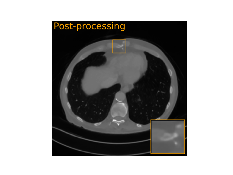
Figure 4.2 shows an example of the different reconstruction methods. We can see that DESYRE is outperformed by the post-processing method. We hypothesize that this is because the post-processing network uses additional information about the inverse problem in training, whereas the training of DESYRE independent of the operator. In comparison to the other regularization methods, DESYRE shows a better performance visually and quantitatively in the case of noise-free data. When comparing DESYRE with the Wavelet synthesis regularization we see that DESYRE does not suffer from the ’pixel-like’ structure even though it is also based on the Haar wavelets. Taking a look at the zoomed in version of the plot, we see that the TV-regularization somehow merges the details, whereas DESYRE is still able to represent these smaller details. One iteration of the wavelet synthesis, TV regularization and DESYRE take $0.057$, $0.051$ and $0.122$ seconds, respectively

To quantitatively compare the reconstructions $u_{\alpha,\delta}$ we compute the peak-signal-to-noise-ration and the normalized-mean-squared-error, respectively

where $u$ is the ground truth. The results of these quantitative comparisons in the case of noise-free data can be seen in Table 4.1.

Figure 4.3 shows an example of the reconstructions using noisy data. In this case DESYRE is able to completely remove the noise from the image. However, it cannot satisfactorily recover any small detail features which are present in the image. When compared to TV-regularization DESYRE shows a more blurry image and is outperformed by the TV-regularization. Like in the noise-free case DESYRE shows a smoother but blurrier image. This suggests that additional regularization, e.g. TV-regularization, of the image should be used to further enhance the image quality. Even though no noise was added during training, the post-processing approach still shows reasonable results. When comparing the two deep learning approaches we see that DESYRE is able to better remove the noise from the image, while the post-processing approach is able to more clearly represent edges.

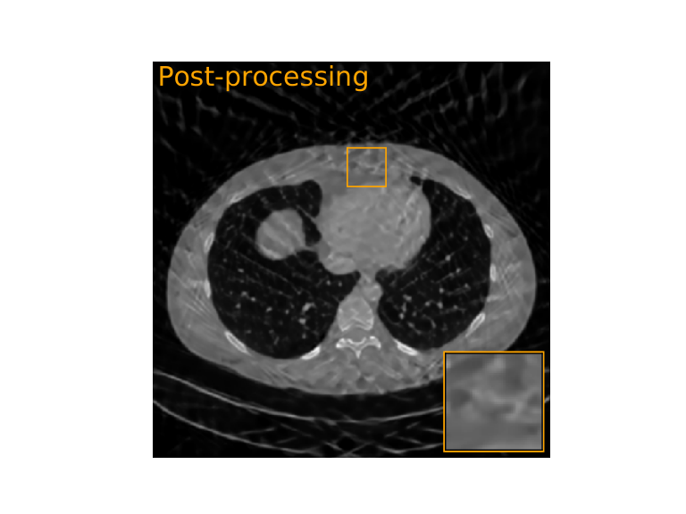
Lastly we illustrate one practical advantage of DESYRE over a standard post-processing approach. To this end, we consider a similar problem as above. However, this time we only take $n_{\theta}=30$ projection views. While the underlying signal class does not change, the reconstruction of the signal is more difficult and the post-processing network trained with $n_{\theta}=60$ has been used. This results in reconstructions containing artefacts (Figure 4.4) which cannot be removed using the post-processing network. Additionally, the post-processing network produces some structure which are not present in the ground truth. While the deep synthesis regularization approach was not able to completely remove the artefacts, it was able to greatly reduce them and does not introduce any additional artefacts. While we have not studied this behaviour in great detail, this suggests that the deep synthesis approach is more generally applicable without retraining the network.

References

- [1] O. Scherzer, M. Grasmair, H. Grossauer, M. Haltmeier, and F. Lenzen, Variational methods in imaging. Springer, 2009.
- [2] H. W. Engl, M. Hanke, and A. Neubauer, Regularization of inverse problems, ser. Mathematics and its Applications. Dordrecht: Kluwer Academic Publishers Group, 1996, vol. 375.
- [3] M. Burger and S. Osher, “Convergence rates of convex variational regularization,” Inverse Probl., vol. 20, no. 5, p. 1411, 2004.
- [4] M. Elad, P. Milanfar, and R. Rubinstein, “Analysis versus synthesis in signal priors,” Inverse Probl., vol. 23, no. 3, p. 947, 2007.
- [5] J. Frikel and M. Haltmeier, “Sparse regularization of inverse problems by operator-adapted thresholding,” arXiv:1909.09364, 2019.
- [6] B. Dong, J. Li, and Z. Shen, “X-ray CT image reconstruction via wavelet frame based regularization and radon domain inpainting,” Journal of Scientific Computing, vol. 54, no. 2-3, pp. 333–349, 2013.
- [7] M. Haltmeier, “Stable signal reconstruction via -minimization in redundant, non-tight frames,” IEEE Trans. Signal Process., vol. 61, pp. 420–426, 2013.
- [8] C. Chaux, P. L. Combettes, J.-C. Pesquet, and V. R. Wajs, “A variational formulation for frame-based inverse problems,” Inverse Problems, vol. 23, no. 4, p. 1495, 2007.
- [9] M. Grasmair, M. Haltmeier, and O. Scherzer, “Sparse regularization with -penalty term,” Inverse Problems, vol. 24, no. 5, p. 055020, 2008.
- [10] Y. Han and J. C. Ye, “Framing U-Net via deep convolutional framelets: Application to sparse-view CT,” IEEE Trans. Med. Imag., vol. 37, pp. 1418–1429, 2018.
- [11] D. Lee, J. Yoo, and J. C. Ye, “Deep residual learning for compressed sensing MRI,” in IEEE 14th International Symposium on Biomedical Imaging, 2017, pp. 15–18.
- [12] J. Adler and O. Öktem, “Solving ill-posed inverse problems using iterative deep neural networks,” Inverse Probl., vol. 33, p. 124007, 2017.
- [13] K. H. Jin, M. T. McCann, E. Froustey, and M. Unser, “Deep convolutional neural network for inverse problems in imaging,” IEEE Trans. Image Process., vol. 26, pp. 4509–4522, 2017.
- [14] H. Li, J. Schwab, S. Antholzer, and M. Haltmeier, “NETT: Solving inverse problems with deep neural networks,” Inverse Problems, 2020, in press.
- [15] J. Rick Chang, C.-L. Li, B. Poczos, B. Vijaya Kumar, and A. C. Sankaranarayanan, “One network to solve them all–solving linear inverse problems using deep projection models,” in Proceedings of the IEEE International Conference on Computer Vision, 2017, pp. 5888–5897.
- [16] Y. Romano, M. Elad, and P. Milanfar, “The little engine that could: Regularization by denoising (RED),” SIAM Journal on Imaging Sciences, vol. 10, no. 4, pp. 1804–1844, 2017.
- [17] S. Lunz, O. Öktem, and C.-B. Schönlieb, “Adversarial regularizers in inverse problems,” in Advances in Neural Information Processing Systems, 2018, pp. 8507–8516.
- [18] H. K. Aggarwal, M. P. Mani, and M. Jacob, “MoDL: model-based deep learning architecture for inverse problems,” IEEE transactions on medical imaging, vol. 38, no. 2, pp. 394–405, 2018.
- [19] D. Obmann, J. Schwab, and M. Haltmeier, “Sparse synthesis regularization with deep neural networks,” arXiv:1902.00390, 2019.
- [20] D. P. Kingma and J. Ba, “Adam: A method for stochastic optimization,” arXiv:1412.6980, 2014.
- [21] C. McCollough, “TU-FG-207A-04: overview of the low dose CT grand challenge,” Medical physics, vol. 43, no. 6, pp. 3759–3760, 2016.
- [22] F. Natterer, The Mathematics of Computerized Tomography. Stuttgart: Teubner, 1986.
- [23] S. Helgason, The Radon transform. Springer, 1999, vol. 2.
- [24] J. Adler, H. Kohr, and O. Öktem, “ODL-a python framework for rapid prototyping in inverse problems,” Royal Institute of Technology, 2017.
- [25] A. Beck and M. Teboulle, “A fast iterative shrinkage-thresholding algorithm for linear inverse problems,” SIAM journal on imaging sciences, vol. 2, no. 1, pp. 183–202, 2009.
- [26] A. Chambolle and T. Pock, “A first-order primal-dual algorithm for convex problems with applications to imaging,” Journal of mathematical imaging and vision, vol. 40, no. 1, pp. 120–145, 2011.