Analysis and optimal control of a malaria mathematical model under resistance and population movement

Cristhian Montoya¹¹ 1 Institute for Mathematical and Computational Engineering. Pontificia Universidad Católica de Chile. Santiago, Chile. cdmontoya85@gmail.com, http://cmontoya.mat.utfsm.cl/ and Jhoana P. Romero--Leiton ²² 2 Universidad de Investigación y Tecnología Experimental Yachay Tech, Urcuquí, Ecuador, jpatirom3@gmail.com

Abstract

In this work, two mathematical models for malaria under resistance are presented. More precisely, the first model shows the interaction between humans and mosquitoes inside a patch under infection of malaria when the human population is resistant to antimalarial drug and mosquitoes population is resistant to insecticides. For the second model, human–mosquitoes population movements in two patches is analyzed under the same malaria transmission dynamic established in one patch. For a single patch, existence and stability conditions for the equilibrium solutions in terms of the local basic reproductive number are developed. These results reveal the existence of a forward bifurcation and the global stability of disease–free equilibrium. In the case of two patches, a theoretical and numerical framework on sensitivity analysis of parameters is presented. After that, the use of antimalarial drugs and insecticides are incorporated as control strategies and an optimal control problem is formulated. Numerical experiments are carried out in both models to show the feasibility of our theoretical results.

Key Words: Insecticides, Antimalarial Drug, Qualitative analysis, Stability, Bifurcation, Resident Budgeting Time Matrix.

1 Introduction

Malaria is a hematoprotozoan parasitic infection transmitted by certain species of anopheline mosquitoes. Four species of plasmodium commonly infect to humans, but one, Plasmodium falciparum is the most lethal in humans, causing many deaths per year. Malaria also provides an unbalance that impairs the economic and social development of certain zones of the planet [17]. In reviewing history, control programs have been focused in two directions: control of the anopheles mosquito through removal of breeding sites, use of insecticides, prevention of contact with humans (by using of screens and bed nets), and use of antimalarial drug (or effective case management) [32]. Unfortunately, the implementation of this control mechanisms has not been entirely effective. Amongst the reasons we can mention: a) resistance of the malaria parasites to antimalarial drugs such as chloroquine and sulfadoxine–pyrimethamine. In this case, and from a mathematical point of view, Aneke in [5] describes the phenomenon of antimalarial drug resistance in a hyperendemic region by a model of ordinary differential equations (ODEs). Esteva et al. in [14] present a deterministic model for monitoring the impact of antimalarial drug resistance on the transmission dynamics of malaria in a human population. Tchuenche et al. in [29] formulate and analyze a mathematical model for malaria with treatment and three levels of resistance in humans incorporing both, sensitive and resistant strains of the parasites. Agusto in [1] formulates and analyzes a deterministic system of ODES for malaria transmission incorporating human movement as well as the development of antimalarial drug resistance in a multipatch–type system. Other works to underline in this topic are [19, 6, 24]. b) The use of pyrethroid insecticides (a man-made pesticides similar to the natural pesticide pyrethrum) in malaria vector control. Here we can find the work of Luz et al. in [22] in which a model of the seasonal population dynamics of Aedes aegypti, both to assess the effectiveness of insecticide interventions on reducing adult mosquito abundance, and to predict evolutionary trajectories of insecticide resistance. In addition, Aldila et al. formulate and analyze a mathematical model for transmission of temephos resistance in Aedes aegypti population [2], meanwhile in the works [3, 16], the authors treat the insecticide resistance in general cases. c) The population migration problem. The movement of infected people or infected mosquitos from areas where malaria is still endemic to areas where the disease had been eradicated led to resurgence of the disease, and this situation also results in a increasing of resistance to insecticides and antimalarial drug [9]. With respect to migration problem, the works have been addressed through multipatch–type models see for instance [15, 26, 1]. Migration problems for dengue virus and other general epidemic models have been reviewed in [18, 8] and [20, 33, 7, 23, 10], respectively.

As far as we know, does not exist mathematical models considering resistance to antimalarial drug and insecticides and movement of populations simultaneously, as factors that hinder the malaria control. Thus, in this paper we give a first response to this situation, including numerical experiments that allow us to verify the feasibility of our theoretical results.

In this paper, we propose two mathematical models for the malaria transmission dynamics and whose equations are based in [27]. More precisely, in the first model, we consider the interaction between humans and mosquitoes inside a patch when the human population is resistant to antimalarial drug and mosquitoes population is resistant to insecticides. Existence and stability conditions for the equilibrium solutions in terms of the local basic reproductive number are determined. For the second model, human–mosquitoes population movements in two patches is considered under the same conditions established in one patch and also following the ideas from [20]. Besides, by incorporating the use of antimalarial drugs and insecticides as control strategies, we formulate an optimal control problem for the disease.

2 One patch model

In this section, we consider a single patch with a susceptible–infected–recovered (SIR) structure for humans and a susceptible–infected (SI) structure for mosquitoes. In order to present the complete model, we describe the dynamic equations that form our model as follows: let us denote as $S_{h}(t)$ , $I_{h}(t)$ and $R_{h}(t)$ the number of susceptible, infected, and recovered humans at time $t$ , respectively. The total human population at time $t$ is denoted by $N_{h}(t)=S_{h}(t)+I_{h}(t)+R_{h}(t)$ . Similarly, let us denote as $S_{v}(t)$ and $I_{v}(t)$ the number of susceptible, and infected mosquitoes at time $t$ , respectively. The total mosquito population at time $t$ is denoted by $N_{v}(t)=S_{v}(t)+I_{v}(t)$ .
Moreover, from [27], we define the force of infection for humans by $\beta_{h}\epsilon\frac{I_{v}}{N_{h}},$ where $\beta_{h}$ represents the probability of a human being infected by the bite of an infected mosquito, and $\epsilon$ represents the per capita biting rate of mosquitoes. Similarly, we define the force of infection for mosquitoes as $\beta_{v}\epsilon\frac{I_{h}}{N_{h}},$ where $\beta_{v}$ represents the probability of infection of mosquito by contact with infected humans.

Respect to susceptible humans population, it is increasing due to recruitment at a constant rate of $\Lambda_{h}$ and by recovered humans from infection, which are represented by the term $\omega R_{h}$ . Simultaneously, this population decrease due to infection by contact with infected mosquitoes through the term $\beta_{h}\epsilon\frac{I_{v}}{N_{h}}S_{h}$ and by natural death through the term $\mu_{h}S_{h}$ . Thus, the ODE that represents the variation of the susceptible humans population is

\dot{S_{h}}=\Lambda_{h}+\omega R_{h}-S_{h}\beta_{h}\epsilon\frac{I_{v}}{N_{h}}-\mu_{h}S_{h},

(2.1)

where the symbol $\cdot$ corresponds to the derivative in time, i.e, $\dot{S_{h}}=\frac{d}{dt}S_{h}(t)$ . Now, respect to the infected humans population, it is treated with drug at a constant rate of $\xi_{1}\theta_{1}$ , where $\xi_{1}$ is the drug efficacy and $\theta_{1}$ is the recovery rate due to the drug. Besides, the number of infected individuals resistant to the drug (by selective pressure) is $\xi_{1}\theta_{1}q_{1}I_{h}$ , where $q_{1}\in[0,1]$ represents the resistance acquisition ratio to the drug. Thus the term $\xi_{1}\theta_{1}(1-q_{1})I_{h}$ represents the proportion of sensitive individuals to the drug. Additionally, a proportion of infected individuals recover spontaneously at a rate of $\delta$ (by action of the immune system), others die from infection at a rate of $\rho$ and others from natural death at a rate of $\mu_{h}$ . Thus, the equation for the variation of the infected humans population is given by

\dot{I}_{h}=S_{h}\beta_{h}\epsilon\frac{I_{v}}{N_{h}}-\xi_{1}\theta_{1}(1-q_{1})I_{h}-(\delta+\rho+\mu_{h})I_{h}.

(2.2)

Finally, in our model the recovered humans population increase by the action of the drug and by spontaneous recovery, and decrease as consequence of natural death and loss of immunity. Thus, the variation of the recovered humans population in time is described by

\dot{R}_{h}=\xi_{1}\theta_{1}(1-q_{1})I_{h}+\delta I_{h}-(\omega+\mu_{h})R_{h}.

(2.3)

On the other hand, the description for the SI model is the following: the susceptible mosquitoes population is recruited at a constant rate of $\Lambda_{v}$ . It is diminished by infection due to contact with infected humans, which is described through the term $\beta_{v}\epsilon\frac{I_{h}}{N_{h}}S_{v}$ . Simultaneously, it is reduced due to natural death with a rate $\mu_{v}$ and by action of insecticides at a rate of $\xi_{2}\theta_{2}$ , where $\xi_{2}$ represents the efficacy of insecticide and $\theta_{2}$ is the death of mosquitoes due to insecticides. The number of mosquitos resistant to the insecticides is $\xi_{2}\theta_{2}q_{2}$ , with $q_{2}\in[0,1]$ represents the resistance acquisition ratio to the insecticides. Thus, the expression $\xi_{2}\theta_{2}(1-q_{2})$ represents the proportion of sensitive mosquitos to the insecticides. Then, the system describing the variation of the mosquitoes population in time is

\left\{\begin{array}[]{ll}&\dot{S_{v}}=\Lambda_{v}-S_{v}\beta_{v}\epsilon\frac{I_{h}}{N_{h}}-\xi_{2}\theta_{2}(1-q_{2})S_{v}-\mu_{v}S_{v}\\ \\ &\dot{I_{v}}=S_{v}\beta_{v}\epsilon\frac{I_{h}}{N_{h}}-\xi_{2}\theta_{2}(1-q_{2})I_{v}-\mu_{v}I_{v}.\end{array}\right.

(2.4)

In summary, from (2.1)-(2.4), our model for malaria under resistance in one patch is given by

\left\{\begin{array}[]{ll}&\dot{S_{h}}=\Lambda_{h}+\omega R_{h}-S_{h}\beta_{h}\epsilon\frac{I_{v}}{N_{h}}-\mu_{h}S_{h}\\ \\ &\dot{I_{h}}=S_{h}\beta_{h}\epsilon\frac{I_{v}}{N_{h}}-\xi_{1}\theta_{1}(1-q_{1})I_{h}-(\delta+\rho+\mu_{h})I_{h}\\ \\ &\dot{R_{h}}=\xi_{1}\theta_{1}(1-q_{1})I_{h}+\delta I_{h}-(\omega+\mu_{h})R_{h}\\ \\ &\dot{S_{v}}=\Lambda_{v}-S_{v}\beta_{v}\epsilon\frac{I_{h}}{N_{h}}-\xi_{2}\theta_{2}(1-q_{2})S_{v}-\mu_{v}S_{v}\\ \\ &\dot{I_{v}}=S_{v}\beta_{v}\epsilon\frac{I_{h}}{N_{h}}-\xi_{2}\theta_{2}(1-q_{2})I_{v}-\mu_{v}I_{v}\\ \\ &(\mathbf{N}_{h}(0),\mathbf{N}_{v}(0))=(S_{h}(0),I_{h}(0).R_{h}(0),S_{v}(0),I_{v}(0)),\end{array}\right.

(2.5)

where $(\mathbf{N}_{h}(0),\mathbf{N}_{v}(0))$ denotes a initial condition and $\mathbf{N}_{h}$ and $\mathbf{N}_{v}$ are vectors formed by $S_{h}$ , $I_{h}$ , $R_{h}$ and $S_{v}$ , $I_{v}$ , respectively.

Remark 2.1.

The novelty in this work involves the parameters $\xi_{i}$ , $\theta_{i}$ and $q_{i}$ with $i=1,2$ . Their interpretation and values are given in Tables 2.1 and 2.2 from Section 2.2. A complete description and interpretation of the others parameters involved in the model (2.5) can be found in [27].

Now, a set of biological interest for the solutions of the system (2.5) is defined as follows

\Omega=\left\{(\mathbf{N}_{h},\mathbf{N}_{v})\in\mathbb{R}_{5}^{+}:\;N_{h}\leq\frac{\Lambda_{h}}{\mu_{h}},\;N_{v}\leq\frac{\Lambda_{v}}{\mu_{v}}\right\}.

(2.6)

The following lemma establishes the invariance property for $\Omega$ .

Lema 2.2.

For $(\mathbf{N}_{h}(0),\mathbf{N}_{v}(0))$ a non–negative initial condition, the system (2.5) has a unique solution and all state variables remain non–negative for all time $t\geq 0$ . Moreover, the set defined on (2.6) is positively invariant with respect the system (2.5).

Proof.

Since the vector field defined on the right side of (2.5) is continuously differentiable, the existence and uniqueness of the solutions is fullfied. On the other hand,

\displaystyle\dot{N_{h}}

\displaystyle=

\displaystyle\Lambda_{h}-\mu_{h}N_{h}-\rho I_{h}\leq\Lambda_{h}-\mu_{h}N_{h}.

Thus

\dot{N_{h}}+\mu_{h}N_{h}\leq\Lambda_{h}.

Multiplying both sides of the above inequality by the integrating factor $e^{\mu_{h}\tau}$ and integrating from $0$ to $t$ , we obtain that

N_{h}(t)\leq N_{h}(0)e^{-\mu_{h}t}+\frac{\Lambda_{h}}{\mu_{h}}(1-e^{-\mu_{h}t}),

from where

\lim_{t\rightarrow\infty}N_{h(t)}\leq\frac{\Lambda_{h}}{\mu_{h}}.

Similar calculation shows that $N_{v}(t)\rightarrow\frac{\Lambda_{v}}{\mu_{v}}$ as $t\rightarrow\infty$ . Thus, the region $\Omega$ is positively invariant. This complete the proof. ∎

2.1 Qualitative analysis

In this subsection, we first compute the local basic reproductive number associated to the system (2.5) . Afterward, conditions for existence and stability of the equilibrium solutions are developed.

2.1.1 Local basic reproductive number

It is well known that a disease–free equilibrium (DFE) is a steady state solution of a system where there is no disease, in our case, $S_{h}=S_{h}^{*}>0$ , $S_{v}=S_{v}^{*}>0$ , and all others variables $I_{h}$ , $I_{v}$ , $R_{h}$ are zero. It will be denoted by $\mathbf{E}_{0_{one}}=\left(\bar{N}_{h},0,0,\bar{N}_{v},0\right)$ , where

\bar{N}_{h}=\frac{\Lambda_{h}}{\mu_{h}},\;\bar{N}_{v}=\frac{\Lambda_{v}}{\xi_{2}\theta_{2}(1-q_{2})+\mu_{v}}\;\text{and}\;\mathbf{E}_{0_{one}}\in\Omega.

(2.7)

Since the basic reproductive number, commonly denoted by $\mathcal{R}_{0}$ (but in this case denoted by $\mathcal{R}_{0_{one}}$ ) is the average number of secondary infective generated by a single infective during the curse of the infection in a whole susceptible population, it is a threshold for determining when an outbreak can occur, or when a disease remains endemic. Using the next generation operator method [30] on the system (2.5), the Jacobian matrices $\mathbf{F}_{one}$ and $\mathbf{V}_{one}$ evaluated in the DFE are given by

\mathbf{F}_{one}=\left(\begin{array}[]{cccc}0&\beta_{h}\epsilon\\ \beta_{v}\epsilon\frac{\bar{N}_{v}}{\bar{N}_{h}}&0\\ \end{array}\right)

and

\mathbf{V}_{one}=\left(\begin{array}[]{cccc}\xi_{1}\theta_{1}(1-q_{1})+\delta+\rho+\mu_{h}&0\\ 0&\xi_{2}\theta_{2}(1-q_{2})+\mu_{v}\\ \end{array}\right).

Thus, the next generator operator of model (2.5) is given by

\mathbf{F}_{one}\mathbf{V}_{one}^{-1}=\left(\begin{array}[]{cccc}0&\frac{\beta_{h}\epsilon}{\xi_{2}\theta_{2}(1-q_{2})+\mu_{v}}\\ \frac{\beta_{v}\epsilon\bar{N}_{v}}{\bar{N}_{h}\left(\xi_{1}\theta_{1}(1-q_{1})+\delta+\rho+\mu_{h}\right)}&0\\ \end{array}\right).

It follows that the local basic reproduction number of the system (2.5), denoted by $\mathcal{R}_{0_{one}}$ is

\mathcal{R}_{0_{one}}=\left(\frac{\beta_{h}\beta_{v}\epsilon^{2}}{\left(\xi_{1}\theta_{1}(1-q_{1})+\delta+\rho+\mu_{h}\right)\left(\xi_{2}\theta_{2}(1-q_{2})+\mu_{v}\right)}\frac{\bar{N}_{v}}{\bar{N}_{h}}\right)^{1/2}.

(2.8)

2.1.2 Existence of endemic equilibria

In this subsection, conditions for existence of endemic equilibria of the model (2.5) are studied. First of all, the existence of the DFE, denoted by $\mathbf{E}_{0_{one}}$ , is guaranteed as consequence of the previous subsection. Now, in order to analyze the endemic equilibria of the model (2.5) we consider the solutions to the algebraic equation system

\left\{\begin{array}[]{rll}\Lambda_{h}+\omega R_{h}-S_{h}\beta_{h}\epsilon\frac{I_{v}}{N_{h}}-\mu_{h}S_{h}&=&0\\ \\ S_{h}\beta_{h}\epsilon\frac{I_{v}}{N_{h}}-\xi_{1}\theta_{1}(1-q_{1})I_{h}-(\delta+\rho+\mu_{h})I_{h}&=&0\\ \\ \xi_{1}\theta_{1}(1-q_{1})I_{h}+\delta I_{h}-(\omega+\mu_{h})R_{h}&=&0\\ \\ \Lambda_{v}-S_{v}\beta_{v}\epsilon\frac{I_{h}}{N_{h}}-\xi_{2}\theta_{2}(1-q_{2})S_{v}-\mu_{v}S_{v}&=&0\\ \\ S_{v}\beta_{v}\epsilon\frac{I_{h}}{N_{h}}-\xi_{2}\theta_{2}(1-q_{2})I_{v}-\mu_{v}I_{v}&=&0.\end{array}\right.

(2.9)

Let us define

\alpha=\frac{\omega}{\omega+\mu_{h}}\frac{\xi_{1}\theta_{1}(1-q_{1})+\delta}{\xi_{1}\theta_{1}(1-q_{1})+\delta+\rho+\mu_{h}}\;\text{where}\;\alpha<1.

(2.10)

Thus, after some algebraic manipulations of the system (2.9), we obtain the following expressions for $S_{h}$ , $R_{h}$ , $S_{v}$ and $I_{v}$ in terms of $I_{h}$

\begin{array}[]{ll}&S_{h}=\frac{\Lambda_{h}}{\mu_{h}}-\frac{\xi_{1}\theta_{1}(1-q_{1})+\delta+\rho+\mu_{h}}{\mu_{h}}(1-\alpha)I_{h}\\ \\ &R_{h}=\frac{\xi_{1}\theta_{1}(1-q_{1})+\delta}{\omega+\mu_{h}}I_{h}\\ \\ &S_{v}=\bar{N}_{v}\left(1-\frac{\beta_{v}\epsilon\bar{N}_{v}}{(\xi_{2}\theta_{2}(1-q_{2})+\mu_{v})\bar{N}_{h}+\left[\beta_{v}\epsilon+\frac{\rho}{\mu_{h}}(\xi_{2}\theta_{2}(1-q_{2})+\mu_{v})\right]}I_{h}\right)\\ \\ &I_{v}=\frac{\beta_{v}\epsilon\bar{N}_{v}}{(\xi_{2}\theta_{2}(1-q_{2})+\mu_{v})\bar{N}_{h}+\left[\beta_{v}\epsilon+\frac{\rho}{\mu_{h}}(\xi_{2}\theta_{2}(1-q_{2})+\mu_{v})\right]}I_{h},\end{array}

(2.11)

and the following cuadratic equation for $I_{h}$

aI_{h}^{2}+bI_{h}+c=0,\;\text{where}

(2.12)

\begin{array}[]{ll}a=&\frac{\rho}{\mu_{h}}\left[\beta_{v}\epsilon+\frac{\rho}{\mu_{h}}\left(\xi_{2}\theta_{2}(1-q_{2})+\mu_{v}\right)\right]\\ \\ b=&a\bar{N}_{h}+\frac{(1-\alpha)\bar{N}_{h}}{\mu_{h}}\left(\xi_{2}\theta_{2}(1-q_{2})+\mu_{v}\right)\left(\xi_{1}\theta_{1}(1-q_{1})+\delta+\rho+\mu_{h}\right)\times\\ \\ &\left[\frac{\rho}{(1-\alpha)(\xi_{1}\theta_{1}(1-q_{1})+\delta+\rho+\mu_{h})}+\mathcal{R}_{0_{one}}^{2}\right]\\ \\ c=&\left(\xi_{2}\theta_{2}(1-q_{2})+\mu_{v}\right)\bar{N}_{h}^{2}\left[1-\mathcal{R}_{0_{one}}^{2}\right].\end{array}

(2.13)

From (2.13), we have e that the coefficients $a$ and $b$ are non–negatives, while $c\geq 0$ if $\mathcal{R}_{0_{one}}^{2}\leq 1$ , otherwise $c<0$ . Thus, the polynomial $P(I_{h})=aI_{h}^{2}+bI_{h}+c$ has only one sign change and by the Descartes’ rule of sign [4] it has one or zero positive roots.
This result is summarized in the following theorem.

Theorem 2.3.

For the model (2.5) always exists the DFE contained in $\Omega$ . Additionally,

1.

If $\mathcal{R}_{0_{one}}\leq 1$ , there are not endemic equilibria.
2.

If $\mathcal{R}_{0_{one}}>1$ there exist one endemic equilibrium .

2.1.3 Stability analysis

In this subsection, we proof the stability of the equilibrium solutions of the system (2.5) given on Theorem 2.3. First, using the linearization of the system (2.5) at the DFE, we proof it local stability, which is determined by the sign of the real part of the eigenvalues of the Jacobian matrix denoted by $J(\mathbf{E}_{0_{one}})$ , which is given by

J(\mathbf{E}_{0_{one}})=\left(\begin{array}[]{ccccc}-\mu_{h}&0&\omega&0&-\beta_{h}\epsilon\\ \\ 0&-\left[\xi_{1}\theta_{1}(1-q_{1})+\delta+\rho+\mu_{h}\right]&0&0&\beta_{h}\epsilon\\ \\ 0&\xi_{1}\theta_{1}(1-q_{1})+\delta&-(\omega+\mu_{h})&0&0\\ \\ 0&-\beta_{v}\epsilon\frac{\bar{N}_{v}}{\bar{N}_{h}}&0&-\left[\xi_{2}\theta_{2}(1-q_{2})+\mu_{v}\right]&0\\ \\ 0&\beta_{v}\epsilon\frac{\bar{N}_{v}}{\bar{N}_{h}}&0&0&-\left[\xi_{2}\theta_{2}(1-q_{2})+\mu_{v}\right]\\ \\ \end{array}\right),

(2.14)

Three eigenvalues of $J(\mathbf{E}_{0_{one}})$ are $\eta_{1}=-\mu_{h}$ , $\eta_{2}=-(\omega+\mu_{h})$ and $\eta_{3}=-\left[\xi_{2}\theta_{2}(1-q_{2})+\mu_{v}\right]$ , while the others eigenvalues are given by the roots of the following quadratic equation

a_{0}\eta^{2}+a_{1}\eta+a_{2}=0,\;\text{where}

(2.15)

$\displaystyle a_{0}$	$\displaystyle=$	$\displaystyle 1$
$\displaystyle a_{1}$	$\displaystyle=$	$\displaystyle\xi_{2}\theta_{2}(1-q_{2})+\mu_{v}+\xi_{1}\theta_{1}(1-q_{1})+\delta+\rho+\mu_{h}$
$\displaystyle a_{2}$	$\displaystyle=$	$\displaystyle\left(\xi_{2}\theta_{2}(1-q_{2})+\mu_{v}\right)\left(\xi_{1}\theta_{1}(1-q_{1})+\delta+\rho+\mu_{h}\right)(1-\mathcal{R}_{0_{one}}^{2}).$

From above, the coefficients $a_{0}$ and $a_{1}$ are positives, while the sign of the coefficient $a_{2}$ depends of $\mathcal{R}_{0_{one}}$ . From the Routh–Hurwitz criterion [13] we can guarantee that the quadratic equation (2.15) has roots with negative real part if and only if its coefficients are positives and the following determinants called minors of Hurwitz are positives

	$\displaystyle\Delta_{1}$	$\displaystyle=$	$\displaystyle a_{1}$
	$\displaystyle\Delta_{2}$	$\displaystyle=$	$\displaystyle\left\|\begin{array}[]{cc}a_{1}&1\\ 0&a_{2}\\ \end{array}\right\|=a_{1}a_{2}.$

We verify that $\Delta_{1}>0$ and $\Delta_{2}>0$ if and only if $\mathcal{R}_{0_{one}}\leq 1$ . In consequence, when $\mathcal{R}_{0_{one}}\leq 1$ the DFE is a locally asymptotically stable (LAS) equilibrium point of the system (2.5).

Now, we are going to proof the stability of the endemic equilibrium of the system (2.5). For this end, we use results based on the center manifold theory described in [11] to show that the system (2.5) exhibits a forward bifurcation when $\mathcal{R}_{0_{one}}=1$ or equivalently when

\beta_{h}\epsilon\doteq\beta^{*}=\frac{\bar{N}_{h}\left(\xi_{2}\theta_{2}(1-q_{2})+\mu_{v}\right)\left(\xi_{1}\theta_{1}(1-q_{1})+\delta+\rho+\mu_{h}\right)}{\beta_{v}\epsilon\bar{N}_{v}}.

(2.17)

The eigenvalues of the Jacobian matrix given on (2.14) evaluated in $(\mathbf{E}_{0_{one}},\beta^{*})$ are $0$ and $-\mu_{h}$ , $-(\omega+\mu_{h})$ , $-\left[\xi_{2}\theta_{2}(1-q_{2})+\mu_{v}\right]$ and $-\left[\xi_{2}\theta_{2}(1-q_{2})+\mu_{v}+\xi_{1}\theta_{1}(1-q_{1})+\delta+\rho+\mu_{h}\right]$ , where the last four have negative real part. In consequence, in $\beta^{*}$ , the DFE is a non–hyperbolic equilibrium. Let $\mathbf{W}=(w_{1},w_{2},w_{3},w_{4},w_{5})^{T}$ a right eigenvector associated to the zero eigenvalue, which satisfies $J(\mathbf{E}_{0_{one}},\beta^{*})\mathbf{W}=0\mathbf{W}=\textbf{0}$ or equivalently

\left\{\begin{array}[]{rl}-\mu_{h}w_{1}+\omega w_{3}-\beta^{*}w_{5}&=0\\ \\ -\left(\xi_{1}\theta_{1}(1-q_{1})+\delta+\rho+\mu_{h}\right)w_{2}+\beta^{*}w_{5}&=0\\ \\ -(\omega+\mu_{h})w_{3}+\frac{\left(\xi_{2}\theta_{2}(1-q_{2})+\mu_{v}\right)\left(\xi_{1}\theta_{1}(1-q_{1})+\delta\right)\bar{N}_{h}}{\beta_{v}\epsilon\bar{N}_{v}}w_{5}&=0\\ \\ -\left(\xi_{2}\theta_{2}(1-q_{2})+\mu_{v}\right)w_{4}-\left(\xi_{2}\theta_{2}(1-q_{2})+\mu_{v}\right)w_{5}&=0.\\ \end{array}\right.

The vectorial form for the solutions of above linear system is given by

\mathbf{W}=\left[\frac{\beta_{h}\epsilon}{\mathcal{R}_{0_{one}}^{2}}(1-\alpha),\frac{\left(\xi_{2}\theta_{2}(1-q_{2})+\mu_{v}\right)\bar{N}_{h}}{\beta_{v}\epsilon\bar{N}_{v}},\frac{\left(\xi_{2}\theta_{2}(1-q_{2})+\mu_{v}\right)\left(\xi_{1}\theta_{1}(1-q_{1})+\delta\right)\bar{N}_{h}}{\beta_{v}\epsilon(\omega+\mu_{h})\bar{N}_{v}},-1,1\right]^{T}w_{5},

(2.18)

where the parameter $\alpha$ is defined on (2.10). Similarly, a left eigenvector $\mathbf{V}=(v_{1},v_{2},v_{3},v_{4},v_{5})$ of the matrix $J(\mathbf{E}_{0_{one}},\beta^{*})$ associated to the zero eigenvalue satisfies that $\mathbf{V}J(\mathbf{E}_{0_{one}},\beta^{*})=0\mathbf{V}=\textbf{0}$ or equivalently $v_{1}=v_{3}=v_{4}=0$ and

\displaystyle\left(\xi_{1}\theta_{1}(1-q_{1})+\delta+\rho+\mu_{h}\right)v_{2}+\beta_{v}\epsilon\frac{\bar{N}_{v}}{\bar{N}_{h}}v_{5}

\displaystyle=

\displaystyle 0,

from where

\mathbf{V}=\left[0,\frac{\beta_{v}\epsilon\bar{N}_{v}}{\bar{N}_{h}\left(\xi_{1}\theta_{1}(1-q_{1})+\delta+\rho+\mu_{h}\right)},0,0,1\right]v_{5}.

(2.19)

The values for $w_{5}$ and $v_{5}$ such that $\mathbf{W}\cdot\mathbf{V}=1$ , are

w_{5}=1\;\text{and}\;v_{5}=\frac{\xi_{1}\theta_{1}(1-q_{1})+\delta+\rho+\mu_{h}}{\xi_{1}\theta_{1}(1-q_{1})+\delta+\rho+\mu_{h}+\xi_{2}\theta_{2}(1-q_{2})+\mu_{v}}.

(2.20)

Thus, the coefficients $\tilde{a}$ and $\tilde{b}$ given on Theorem 4.1 from [11]

\begin{array}[]{ll}\tilde{a}=&\frac{1}{2}\sum_{k,i,j=1}^{5}v_{k}w_{i}w_{j}\frac{\partial^{2}f_{k}}{\partial x_{i}\partial x_{j}}(\mathbf{E}_{0_{one}},\beta^{*})\\ \\ \tilde{b}=&\sum_{k,i=1}^{5}v_{k}w_{i}\frac{\partial^{2}f_{k}}{\partial x_{i}\partial\beta^{*}}(\mathbf{E}_{0_{one}},\beta^{*}),\end{array}

(2.21)

can be explicitly computed as follows. Let us denote as $f_{i}$ , $i=1,...,5$ to the scalar functions of the right hand of the system (2.5), and $x_{1}=S_{h}$ , $x_{2}=I_{h}$ , $x_{3}=R_{h}$ , $x_{4}=S_{v}$ , $x_{5}=I_{v}$ . The coefficients $w_{p}$ and $v_{p}$ with $p=1,2,...5$ of (2.21), represent to the components of the eigenvectors $\mathbf{W}$ and $\mathbf{V}$ defined on (2.18) and (2.19), respectively. After some calculations we have that the second order partial derivatives evaluated in $(\mathbf{E}_{0_{one}},\beta^{*})$ are given by

\begin{array}[]{lll}\frac{\partial^{2}f_{1}}{\partial x_{5}\partial x_{2}}=\frac{\partial^{2}f_{1}}{\partial x_{5}\partial x_{3}}=\frac{\beta_{h}\epsilon}{\bar{N}_{h}}&\frac{\partial^{2}f_{5}}{\partial x_{2}\partial x_{1}}=\frac{\partial^{2}f_{5}}{\partial x_{2}\partial x_{3}}=\frac{-\beta_{v}\epsilon\bar{N}_{v}}{\bar{N}_{h}^{2}}&\frac{\partial^{2}f_{2}}{\partial x_{5}\partial x_{2}}=\frac{\partial^{2}f_{2}}{\partial x_{5}\partial x_{3}}=-\frac{\beta_{h}\epsilon}{\bar{N}_{h}}\\ \\ \frac{\partial^{2}f_{4}}{\partial x_{2}\partial x_{1}}=\frac{\beta_{v}\epsilon\bar{N}_{v}}{\bar{N}_{h}^{2}}&\frac{\partial^{2}f_{4}}{\partial x_{2}\partial x_{4}}=-\frac{\beta_{v}\epsilon}{\bar{N}_{h}}&\frac{\partial^{2}f_{5}}{\partial x_{2}\partial x_{4}}=\frac{\beta_{v}\epsilon}{\bar{N}_{h}}\\ \\ \frac{\partial^{2}f_{4}}{\partial x_{2}^{2}}=\frac{2\beta_{v}\epsilon\bar{N}_{v}}{\bar{N}_{h}^{2}}&\frac{\partial^{2}f_{5}}{\partial x_{2}^{2}}=-\frac{2\beta_{v}\epsilon\bar{N}_{v}}{\bar{N}_{h}^{2}}.&\end{array}

In the above expressions we did not consider to the zero and cross partial derivatives. Additionally, the second order partial derivatives with respect to the bifurcation parameter $\beta^{*}$ evaluated in $\mathbf{E}_{0_{one}}$ are all zero except

\frac{\partial^{2}f_{1}}{\partial x_{5}\partial\beta^{*}}=-1\quad\text{and}\quad\frac{\partial^{2}f_{2}}{\partial x_{5}\partial\beta^{*}}=1.

Thus, the coefficients $\tilde{a}$ and $\tilde{b}$ given on (2.21) can be expressed as

\begin{array}[]{ll}\tilde{a}&=2\frac{\partial^{2}f_{2}}{\partial x_{5}\partial x_{2}}v_{2}(w_{2}+w_{3})+2\frac{\partial^{2}f_{5}}{\partial x_{1}\partial x_{2}}w_{2}(w_{1}+w_{3})-\frac{\partial^{2}f_{5}}{\partial x_{2}\partial x_{4}}w_{2}+\frac{1}{2}\frac{\partial^{2}f_{5}}{\partial x_{2}^{2}}w_{2}^{2}\\ \\ &=-\frac{2\beta^{*}}{\bar{N}_{h}}v_{2}(w_{2}+w_{3})-\frac{2\beta_{v}\epsilon\bar{N}_{v}}{\bar{N}_{h}^{2}}w_{2}(w_{1}+w_{3})-\frac{\beta_{v}\epsilon}{\bar{N}_{h}}w_{2}-\frac{\beta_{v}\epsilon\bar{N}_{v}}{\bar{N}_{h}^{2}}w_{2}^{2}\\ \\ \tilde{b}&=v_{2}w_{5}\frac{\partial^{2}f_{2}}{\partial x_{5}\partial\beta^{*}}=\frac{\beta_{v}\epsilon\bar{N}_{v}}{\bar{N}_{h}\left(\xi_{1}\theta_{1}(1-q_{1})+\delta+\rho+\mu_{h}+\xi_{2}\theta_{2}(1-q_{2})+\mu_{v}\right)}.\end{array}

(2.22)

From (2.22) we have that $\tilde{b}>0$ while the sign of $\tilde{a}$ depends of the sign of $w_{2}$ , $v_{2}(w_{2}+w_{3})$ and $w_{2}(w_{1}+w_{3})$ . From (2.18) and (2.19) we verify that $w_{2}\geq 0$ , $v_{2}(w_{2}+w_{3})\geq 0$ , and

w_{2}(w_{1}+w_{3})=w_{2}\left[\frac{\beta_{h}\epsilon}{\mathcal{R}_{0_{one}}^{2}}(1-\alpha)+\frac{\left(\xi_{2}\theta_{2}(1-q_{2})+\mu_{v}\right)\left(\xi_{1}\theta_{1}(1-q_{1})+\delta\right)\bar{N}_{h}}{\beta_{v}\epsilon(\omega+\mu_{h})\bar{N}_{v}}\right]\geq 0.

Thus, by Theorem 4.1 from [11], the endemic equilibrium is LAS when $\mathcal{R}_{0_{one}}>1$ , which suggest the global stability of the DFE. The previous results are summarized in the following theorem.

Theorem 2.4.

If $\mathcal{R}_{0_{one}}\leq 1$ the DFE is LAS in $\Omega$ , and the endemic equilibrium is unestable. If $\mathcal{R}_{0_{one}}>1$ the DFE becomes an unstable hyperbolic equilibrium point, and the endemic equilibrium is LAS in $\Omega$ .

Figure 2.1 shows the bifurcation diagram.

Figure 2.1: A forward bifurcation occurs when

\mathcal{R}_{0_{one}}=1

Theorem 2.5.

If $\mathcal{R}_{0_{one}}^{2}\leq 1$ , then the DFE is globally asymptotically (GAS) stable in $\Omega$ .

Proof.

From Theorem 2.4, when $\mathcal{R}_{0_{one}}^{2}\leq 1$ , the $DFE$ is LAS in $\Omega$ . Let $(\mathbf{N}_{h}(t),\mathbf{N}_{v}(t))$ a positive solution of the system (2.5), then by Lemma 2.2 it satisfies that

S_{v}(t)\leq\bar{N}_{v}(t)\;\text{and}\;N_{h}(t)>\frac{\Lambda_{h}}{\rho+\mu_{h}}.

(2.23)

We will proof the existence of a Lyapunov function for the traslated system $\dot{\mathbf{y}}=f(\mathbf{y}+\mathbf{E}_{0_{one}})-f(\mathbf{E}_{0_{one}})=F(\mathbf{y})$ , where $f$ is the vectorial field defined from right hand of the system (2.5) and $\mathbf{y}=\mathbf{0}$ is a trivial solution of the system $\dot{\mathbf{y}}=F(\mathbf{y})$ . Let us consider the following function

V^{*}(\mathbf{N}_{h},\mathbf{N}_{v})=\frac{\beta_{h}\epsilon}{\xi_{2}\theta_{2}(1-q_{2})+\mu_{v}}I_{v}+I_{h},

and let

V(\tilde{\mathbf{N}}_{h},\tilde{\mathbf{N}}_{v})=V^{*}(S_{h}-\bar{N}_{h},I_{h},R_{h},S_{v}-\bar{N}_{v},I_{v}).

(2.24)

The function $V$ defined on (2.24) satisfies the following properties

(P1)

$V(\bar{N}_{h},0,0,\bar{N}_{v},0)=V(\mathbf{E}_{0_{one}})=V^{*}(\mathbf{0})=0$ .
(P2)

$V>0$ $\forall(\tilde{\mathbf{N}_{h}},\tilde{\mathbf{N}_{v}})\neq\mathbf{E}_{0_{one}}$ in $\Omega$ (V is positive definite).

(P3)

The orbital derivative of $V$ along the trajectories of (2.5) is negative definite. In fact,

$\displaystyle\dot{V}$	$\displaystyle=$	$\displaystyle\frac{\partial V^{}}{\partial(S_{h}-\bar{N}_{h})}f_{1}+\frac{\partial V^{}}{\partial I_{h}}f_{2}+\frac{\partial V^{}}{\partial R_{h}}f_{3}+\frac{\partial V^{}}{\partial(S_{v}-\bar{N}_{v})}f_{4}+\frac{\partial V^{*}}{\partial I_{v}}$
	$\displaystyle=$	$\displaystyle S_{h}\beta_{h}\epsilon\frac{I_{v}}{N_{h}}-\xi_{1}\theta_{1}(1-q_{1})I_{h}-(\delta+\rho+\mu_{h})I_{h}+$
		$\displaystyle\frac{\beta_{h}\epsilon}{\xi_{2}\theta_{2}(1-q_{2})+\mu_{v}}\left(S_{v}\beta_{v}\epsilon\frac{I_{h}}{N_{h}}-\xi_{2}\theta_{2}(1-q_{2})I_{v}-\mu_{v}I_{v}\right)$
	$\displaystyle=$	$\displaystyle\left[\frac{S_{v}\beta_{h}\beta_{v}\epsilon^{2}}{N_{h}\left(\xi_{2}\theta_{2}(1-q_{2})+\mu_{v}\right)}-\left(\xi_{1}\theta_{1}(1-q_{1})+\delta+\rho+\mu_{h}\right)\right]I_{h}$
		$\displaystyle+\left[\beta_{h}\epsilon\frac{S_{h}}{N_{h}}-\beta_{h}\epsilon\right]I_{v}$
	$\displaystyle\leq$	$\displaystyle\left(\xi_{1}\theta_{1}(1-q_{1})+\delta+\rho+\mu_{h}\right)\left[\mathcal{R}_{0_{one}}^{2}-1\right]I_{h}\leq 0.$

Thus, the DFE is globally stable in $\Omega$ . To verify its global asymptotic stability, let us consider $\triangle=\{(\mathbf{N}_{h},\mathbf{N}_{v}):\dot{V}=0\}$ . Then $\triangle\subset\{(\mathbf{N}_{h},\mathbf{N}_{v}):I_{h}=0\}$ . Let $\triangle^{\prime}\subset\triangle$ the biggest invariant set with respect to (2.5) and $(\mathbf{N}_{h},\mathbf{N}_{v})$ a solution of (2.5) in $\triangle^{\prime}$ , then $(\mathbf{N}_{h},\mathbf{N}_{v})$ is defined and is bounded $\forall t\in\mathbb{R}$ and $I_{h}(t)=0$ in $\triangle^{\prime}$ for all $t$ . Replacing this value in the system (2.5) we obtain that $R_{h}(t)=I_{v}(t)=0$ for all $t$ , while from the first and fourth equation of (2.5) we obtain that $S_{h}(t)=\Lambda_{h}/\mu_{h}=\bar{N}_{h}$ and $S_{v}(t)=\Lambda_{v}/(\xi_{2}\theta_{2}(1-q_{2})+\mu_{v})=\bar{N}_{v}$ . Thus, $\triangle^{\prime}=\{\mathbf{E}_{0_{one}}\}$ and from the Lasalle invariance principle [31] $\mathbf{E}_{0_{one}}$ is GAS in $\Omega$ . ∎

2.2 Numerical experiments

In this subsection, we validate our theoretical results with numerical experiments. For this end, we take data from rural areas of Tumaco (Colombia) reported in [27] and make some numerical simulations. For the values of the parameters corresponding to insecticides, we assume that the fumigation is done with two pyrethroids insecticides (deltamethrin and cyfluthrin) according to the recommendations of Palomino et al. in [25]. Pyrethroids insecticides are a special chemicals class of active ingredients found in many of the modern insecticides used by pest management professionals. Due to the low concentrations in which these products are applied, a constant safety of use and a decrease in the toxic impact on vector control have been achieved. For the values of the parameters corresponding to the drug, we assume that the infected patients are treated with artemisinin–based combination therapy (ACT) according to the recomendations of Smith in [28]. Artemisinin (also called qinghaosu), is an antimalarial drug derived from the sweet wormwood plant: Artemisia annua. Fast acting artemisinin–based compounds are combined with other drugs, for example, lumefantrine, mefloquine, amodiaquine, sulfadoxine/pyrimethamine, piperaquine and chlorproguanil/dapsone. The artemisinin derivatives include dihydroartemisinin, artesunate and artemether [28]. Tables 2.1 and 2.2 show the values of the parameters corresponding to the drugs and insecticides supply, respectively.

Table 2.1: Values of the parameters corresponding to the ACT supply.

Parameter	Interpretation	Dimension	Value
$\xi_{1}$	Drug efficacy	Dimensionless	0.7
$\theta_{1}$	Recovery rate due to the drug	Day^-1	0.6
$q_{1}$	Resistance acquisition ratio to the drug	Dimensionless	0.1

Table 2.2: Values of the parameters corresponding to insecticides supply.

Parameter	Interpretation	Dimension
$\xi_{2}$	Insecticide efficacy	Dimensionless
$\theta_{2}$	Death rate due to the insecticides	Day ^-1
$q_{2}$	Resistance acquisition ratio to the insecticides	Dimensionless
	Value for deltamethrin	Value for cyfluthrin
	0.7	0.2
	0.3	0.3
	0.05	0.2

Figure 2.2 shows the behavior of human and mosquito populations when the patients are treated with ACT and the mosquitoes are fumigated with cyfluthrin and deltamethrin, respectively. In Figure 2.2 (a) the solutions tend to an endemic equilibrium and $\mathcal{R}_{0_{one}}^{2}=2.15$ , while in Figure 2.2 (b) the solutions tend to the DFE and $\mathcal{R}_{0_{one}}^{2}=0.0012$ . In fact, given that cyfluthrin is an insectcide with less efficacy than deltamethrin, its application generates greater resistance hindering the disease control.

Refer to caption — (a) Fumigation with cyfluthrin

In Figure 2.3 we consider the effects of resistance in the population dynamics. In Figures 2.3 (a) and (b) we assume that there is no resistance ( $q_{1}=q_{2}=0$ ). Then, when the fumigation is done with cyflutrin, $\mathcal{R}_{0_{one}}^{2}=1.41$ and the solutions tend to the endemic equilibrium (8136, 227, 1541, 250, 32), which evidences a considerable reduction in the persistence of the infection, while if the fumigation is done with deltamethrin, $\mathcal{R}_{0_{one}}^{2}=0.00095$ and the solutions tend to the DFE. In Figures 2.3 (c) and (d) we assume total resistance ( $q_{1}=q_{2}=1$ ). Then, when the fumigation is done with cyflutrin, $\mathcal{R}_{0_{one}}^{2}=2724.4$ and the solutions tend to the endemic equilibrium (0, 789, 0, 0, 4699), which evidences that after the first 30 days, all individuals (humans and mosquitoes) will be infected, while if the fumigation is done with deltamethrin, $\mathcal{R}_{0_{one}}^{2}=264.8$ and the solutions tend to the endemic equilibrium (6, 824, 0, 195, 4617), which evidences a persistence of the infection.

3 Two patch model

In this section we model the malaria transmission dynamics between humans and mosquitoes within a patch and their spatial dispersal between two patches. Within a single patch, our model is defined by the equations (2.5), where the subscripts $1$ and $2$ refers to patch $1$ and patch $2$ , respectively. The patches are coupled via the resident budgeting time matrix $\mathbf{R}=[\lambda_{ij}]_{2\times 2}$ for $i,j=1,2$ as in [20]. Here $\lambda_{ij}\doteq\alpha_{ij}+\beta_{ji}$ , being $\alpha_{ij}$ the probability of a human from patch $i$ is visiting the patch $j$ and $\beta_{ji}$ the probability of a mosquito from patch $j$ , is visiting the patch $i$ . Some authors prefer not to consider the mobility of mosquitoes due to yours short life cycle (less than two weeks without captivity), in which case we assume $\beta_{ji}=0$ . Each $\lambda_{ij}$ is a constant in $[0,1]$ and $\sum_{j=1}^{2}\lambda_{ij}=1$ for $i=1,2$ . In this model we include bi–directional motion as in [20], that is, a susceptible human (mosquito) in patch $i$ can be infected by an infected mosquito (human) from patch $i$ as well as by an infected mosquito (human) from patch $j$ who is visiting the patch $i$ . Thus, the dynamic in two patches are represented through the following system of nonlinear ODEs:

\left\{\begin{array}[]{ll}&\dot{S_{h_{i}}}=\Lambda_{h_{i}}+\omega_{i}R_{h_{i}}-S_{h_{i}}\sum_{j=1}^{2}\lambda_{ij}\beta_{hj}\epsilon_{j}\frac{I_{v_{j}}}{N_{h_{j}}}-\mu_{h_{i}}S_{h_{i}}\\ \\ &\dot{I_{h_{i}}}=\sum_{j=1}^{2}\lambda_{ij}\beta_{hj}\epsilon_{j}\frac{I_{v_{j}}}{N_{h_{j}}}-\xi_{1i}\theta_{1i}(1-q_{1i})I_{h_{i}}-(\delta_{i}+\rho_{i}+\mu_{h_{i}})I_{h_{i}}\\ \\ &\dot{R_{h_{i}}}=\xi_{1i}\theta_{1i}(1-q_{1i})I_{h_{i}}+\delta_{i}I_{h_{i}}-(\omega_{i}+\mu_{h_{i}})R_{h_{i}}\\ \\ &\dot{S_{v_{i}}}=\Lambda_{v_{i}}-S_{v_{i}}\sum_{j=1}^{2}\lambda_{ji}\beta_{vj}\epsilon_{j}\frac{I_{h_{j}}}{N_{h_{j}}}-\xi_{2i}\theta_{2i}(1-q_{2i})-\mu_{v_{i}}S_{v_{i}}\\ \\ &\dot{I_{v_{i}}}=S_{v_{i}}\sum_{j=1}^{2}\lambda_{ji}\beta_{vj}\epsilon_{j}\frac{I_{h_{j}}}{N_{h_{j}}}-\xi_{2i}\theta_{2i}(1-q_{2i})-\mu_{v_{i}}I_{v_{i}},\quad\text{for}\quad i=1,2\\ \\ &(\mathbf{N}_{h_{1}}(0),\mathbf{N}_{v_{1}}(0),\mathbf{N}_{h_{2}}(0),\mathbf{N}_{v_{2}}(0))=(\mathbf{N}_{h_{1}}^{0},\mathbf{N}_{v_{1}}^{0},\mathbf{N}_{h_{2}}^{0},\mathbf{N}_{v_{2}}^{0}),\end{array}\right.

(3.1)

where $(\mathbf{N}_{h_{1}}(0),\mathbf{N}_{v_{1}}(0),\mathbf{N}_{h_{2}}(0),\mathbf{N}_{v_{2}}(0))$ denotes an initial condition. Let us define $N_{H}(t)=N_{h_{1}}(t)+N_{h_{2}}(t)$ , $N_{V}(t)=N_{v_{1}}(t)+N_{v_{2}}(t)$ and

\begin{array}[]{ll}\Lambda_{H}=2\max\{\Lambda_{h_{1}},\;\Lambda_{h_{2}}\},&\mu_{H}=\min\{\mu_{h_{1}},\;\mu_{h_{2}}\}\\ \Lambda_{V}=2\max\{\Lambda_{v_{1}},\;\Lambda_{v_{2}}\},&\mu_{V}=\min\{\mu_{v_{1}},\;\mu_{v_{2}}\}.\end{array}

(3.2)

A set of biological interest for the solutions of the system (3.1) is

\bar{\Omega}=\left\{(\mathbf{N}_{h_{1}},\mathbf{N}_{v_{1}},\mathbf{N}_{h_{2}},\mathbf{N}_{v_{2}})\in\mathbb{R}_{10}^{+}:\;N_{H}\leq\frac{\Lambda_{H}}{\mu_{H}}\;\text{and}\,N_{V}\leq\frac{\Lambda_{V}}{\mu_{V}}\right\}.

(3.3)

The proof of invariance of $\bar{\Omega}$ can be be made using the results of Lemma 2.2.

3.1 Global basic reproductive number and numerical experiments

In this subsection, we first compute the global basic reproductive number associated to the system (3.1). Then, we obtain numerical experiments to generate an application of the mathematical model (3.1) using data from [27]. Let us denote as $\mathbf{E}_{0}=\left(\bar{N}_{h_{1}},0,0,\bar{N}_{v_{1}},0,\bar{N}_{h_{2}},0,0,\bar{N}_{v_{2}},0\right)$ with

\bar{N}_{h_{i}}=\frac{\Lambda_{h_{i}}}{\mu_{h_{i}}}\;\text{and}\;\bar{N}_{v_{i}}=\frac{\Lambda_{v_{i}}}{\xi_{2i}\theta_{2i}(1-q_{2i})+\mu_{v_{i}}}\;\text{for}\;i=1,2,

(3.4)

to the DFE associated to the system (3.1). Using a similar procedure to that Subsection 2.1.1 with

\mathbf{F}=\left(\begin{array}[]{cccc}0&\lambda_{11}\beta_{h_{1}}\epsilon_{1}&0&\lambda_{12}\beta_{h_{2}}\epsilon_{2}\frac{\bar{N}_{h_{1}}}{\bar{N}_{h_{2}}}\\ \lambda_{11}\beta_{v_{1}}\epsilon_{1}\frac{\bar{N}_{v_{1}}}{\bar{N}_{h_{1}}}&0&\lambda_{21}\beta_{v_{1}}\epsilon_{2}\frac{\bar{N}_{v_{1}}}{\bar{N}_{h_{2}}}&0\\ 0&\lambda_{21}\beta_{h_{1}}\epsilon_{1}\frac{\bar{N}_{h_{2}}}{\bar{N}_{h_{1}}}&0&\lambda_{22}\beta_{h_{2}}\epsilon_{2}\\ \lambda_{12}\beta_{v_{1}}\epsilon_{1}\frac{\bar{N}_{v_{2}}}{\bar{N}_{h_{1}}}&0&\lambda_{22}\beta_{v_{2}}\epsilon_{2}\frac{\bar{N}_{v_{2}}}{\bar{N}_{h_{2}}}&0\\ \end{array}\right)\;\text{and}

\mathbf{V}=\left(\begin{array}[]{cccc}\xi_{11}\theta_{11}(1-q_{11})+\delta_{1}+\rho_{1}+\mu_{h_{1}}&0&0&0\\ \\ 0&\xi_{21}\theta_{21}(1-q_{21})+\mu_{v_{1}}&0&0\\ \\ 0&0&\xi_{12}\theta_{12}(1-q_{12})+\delta_{2}+\rho_{2}+\mu_{h_{2}}&0\\ \\ 0&0&0&\xi_{22}\theta_{22}(1-q_{22})+\mu_{v_{2}}\\ \end{array}\right),

we get the following expression to the global basic reproductive number

\mathcal{R}_{0}=\left(\frac{\eta_{1}+\sqrt{\eta_{2}}}{2}\right)^{1/2},

(3.5)

where

\begin{array}[]{ll}\eta_{1}&=\frac{\beta_{h_{1}}\epsilon_{1}}{\xi_{21}\theta_{21}(1-q_{21})+\mu_{v_{1}}}\frac{\bar{N}_{v_{1}}}{\bar{N}_{h_{1}}}\left[\frac{\lambda_{21}^{2}\beta_{v_{2}}\epsilon_{2}}{\left(\xi_{12}\theta_{12}(1-q_{12})+\delta_{2}+\rho_{2}+\mu_{h_{2}}\right)}+\frac{\lambda_{11}^{2}\beta_{v_{1}}\epsilon_{1}}{\left(\xi_{11}\theta_{11}(1-q_{11})+\delta_{1}+\rho_{1}+\mu_{h_{1}}\right)}\right]\\ \\ &+\frac{\beta_{h_{2}}\epsilon_{2}}{\xi_{22}\theta_{22}(1-q_{22})+\mu_{v_{2}}}\frac{\bar{N}_{v_{2}}}{\bar{N}_{h_{2}}}\left[\frac{\lambda_{12}^{2}\beta_{v_{1}}\epsilon_{1}}{\left(\xi_{11}\theta_{11}(1-q_{11})+\delta_{1}+\rho_{1}+\mu_{h_{1}}\right)}+\frac{\lambda_{22}^{2}\beta_{v_{2}}\epsilon_{2}}{\left(\xi_{12}\theta_{12}(1-q_{12})+\delta_{2}+\rho_{2}+\mu_{h_{2}}\right)}\right]\\ \\ \eta_{2}&=\left[\frac{\lambda_{11}^{2}\beta_{v_{1}}\beta_{h_{1}}\epsilon_{1}^{2}}{\left(\xi_{21}\theta_{21}(1-q_{21})+\mu_{v_{1}}\right)\left(\xi_{11}\theta_{11}(1-q_{11})+\delta_{1}+\rho_{1}+\mu_{h_{1}}\right)}\frac{\bar{N}_{v_{1}}}{\bar{N}_{h_{1}}}\right.\left.+\frac{\lambda_{12}^{2}\beta_{v_{2}}\beta_{h_{2}}\epsilon_{2}^{2}}{\left(\xi_{22}\theta_{22}(1-q_{22})+\mu_{v_{2}}\right)\left(\xi_{12}\theta_{12}(1-q_{12})+\delta_{2}+\rho_{2}+\mu_{h_{2}}\right)}\frac{\bar{N}_{v_{2}}}{\bar{N}_{h_{2}}}\right]^{2}\\ \\ &+\left[\frac{\lambda_{21}^{2}\beta_{v_{1}}\beta_{h_{1}}\epsilon_{1}\epsilon_{2}}{\left(\xi_{21}\theta_{21}(1-q_{21})+\mu_{v_{1}}\right)\left(\xi_{11}\theta_{11}(1-q_{11})+\delta_{1}+\rho_{1}+\mu_{h_{1}}\right)}\frac{\bar{N}_{v_{1}}}{\bar{N}_{h_{1}}}\right.\left.+\frac{\lambda_{22}^{2}\beta_{v_{2}}\beta_{h_{2}}\epsilon_{2}^{2}}{\left(\xi_{22}\theta_{22}(1-q_{22})+\mu_{v_{2}}\right)\left(\xi_{12}\theta_{12}(1-q_{12})+\delta_{2}+\rho_{2}+\mu_{h_{2}}\right)}\frac{\bar{N}_{v_{2}}}{\bar{N}_{h_{2}}}\right]^{2}\\ \\ &+2\frac{\beta_{v_{1}}\beta_{v_{2}}\epsilon_{1}\epsilon_{2}}{\left(\xi_{11}\theta_{11}(1-q_{11})+\delta_{1}+\rho_{1}+\mu_{h_{1}}\right)\left(\xi_{12}\theta_{12}(1-q_{12})+\delta_{2}+\rho_{2}+\mu_{h_{2}}\right)}\times\left[\frac{\lambda_{12}^{2}\lambda_{22}^{2}\beta_{h_{2}}^{2}\epsilon_{2}^{2}\bar{N}_{v_{2}}^{2}}{\left(\xi_{22}\theta_{22}(1-q_{22})+\mu_{v_{2}}\right)^{2}\bar{N}_{h_{2}}^{2}}+\frac{\lambda_{11}^{2}\lambda_{21}^{2}\beta_{h_{1}}^{2}\epsilon_{1}^{2}\bar{N}_{v_{1}}^{2}}{\left(\xi_{21}\theta_{21}(1-q_{21})+\mu_{v_{1}}\right)^{2}\bar{N}_{h_{1}}^{2}}\right]\\ \\ &+2\frac{\beta_{h_{1}}\beta_{h_{2}}\beta_{v_{1}}\beta_{v_{2}}\epsilon_{1}^{2}\epsilon_{2}^{2}}{\left(\xi_{21}\theta_{21}(1-q_{21})+\mu_{v_{1}}\right)\left(\xi_{11}\theta_{11}(1-q_{11})+\delta_{1}+\rho_{1}+\mu_{h_{1}}\right)\left(\xi_{22}\theta_{22}(1-q_{22})+\mu_{v_{2}}\right)\left(\xi_{12}\theta_{12}(1-q_{12})+\delta_{2}+\rho_{2}+\mu_{h_{2}}\right)}\\ \\ &\times\frac{\bar{N}_{v_{1}}\bar{N}_{v_{2}}}{\bar{N}_{h_{1}}\bar{N}_{h_{2}}}\left[4\lambda_{11}\lambda_{12}\lambda_{21}\lambda_{22}-\lambda_{11}^{2}\lambda_{22}^{2}-\lambda_{12}^{2}\lambda_{21}^{2}\right].\end{array}

Considering the uncopling system (that is, $\lambda_{11}=1$ and $\lambda_{22}=1$ ) in (3.5), we obtain the local basic reproductive number for each patch given in (2.8).

In what follows, we make some numerical experiments. For this purpose, we are going to consider the following hypothesis: (a) the patch 1 and patch 2 represent rural areas (RA) and urban areas (UA) from the municipality of Tumaco (Colombia) as in [27, leiton2018analisis], respectively. (b) The epidemiological outbreak begins in RA and the individuals in UA acquire the infection due to the coupling between the two patches. Therefore (unless otherwise stated), the initial condition will be $S_{h_{1}}(0)=100000$ , $I_{h_{1}}(0)=30000$ , $R_{h_{1}}(0)=20000$ , $S_{v_{1}}(0)=50000$ , $I_{v_{1}}(0)=10000$ , $S_{h_{2}}(0)=100000$ , $S_{v_{2}}(0)=50000$ and all others zero. (c) Mosquitos are fumigated only with cyflutrin (data from Table 2.2). (d) The infected patient are treated with ACT (data from Table 2.1). (d) The resistance acquisition ratio in RA is higher than UA due to in RA individuals are continuously exposed to the parasite, that is, $q_{11}=0.1$ , $q_{12}=0.09$ , $q_{21}=0.05$ and $q_{22}=0.04$ . Besides, we will consider the following coupling scenarios poposed by Lee et al. in [20]:

(S1)

Uncoupled: when there are no visits between patches, that is, $\lambda_{11}=\lambda_{22}=1$ and others are equal to zero
(S2)

Weakly–coupling: small values for $\lambda_{12}$ and $\lambda_{21}$ .
(S3)

Strongly–coupling: when visitors from patch 2 spend quite an amount of time in patch 1, that is, $\lambda_{22}<\lambda_{11}$ .

Table 3.1 shows the values of the parameters in the residence–time matrix considering different scenarios of coupling.

Table 3.1: Values of the parameters in the residence–time matrix.

Scenario	Values of the parameters
Uncoupled	$\lambda_{11}=\lambda_{22}=1$ , $\lambda_{12}=\lambda_{21}=0$
Weakly–coupling	$\lambda_{11}=\lambda_{22}=0.9$ , $\lambda_{12}=\lambda_{21}=0.1$
Strongly–coupling	$\lambda_{11}=\lambda_{22}=0.4$ , $\lambda_{12}=\lambda_{21}=0.6$

Figure 3.1 shows the behavior of the solutions when the system (3.1) is uncoupled. If the disease begins in patch 1, the disease does not spread to patch 2.

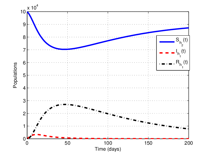
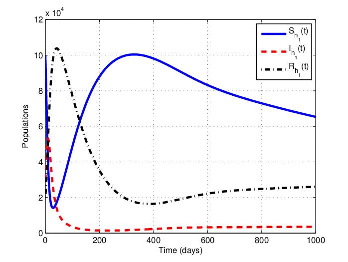
Figure 3.2 shows the behavior of the humans and mosquitoes populations in patches 1 and 2, respectively, considering weakly–coupling. Here, the disease is spread from patch 1 to patch 2 during the first 50 days, then the disease is eliminated in patch 2, and remains at low load in patch 1.

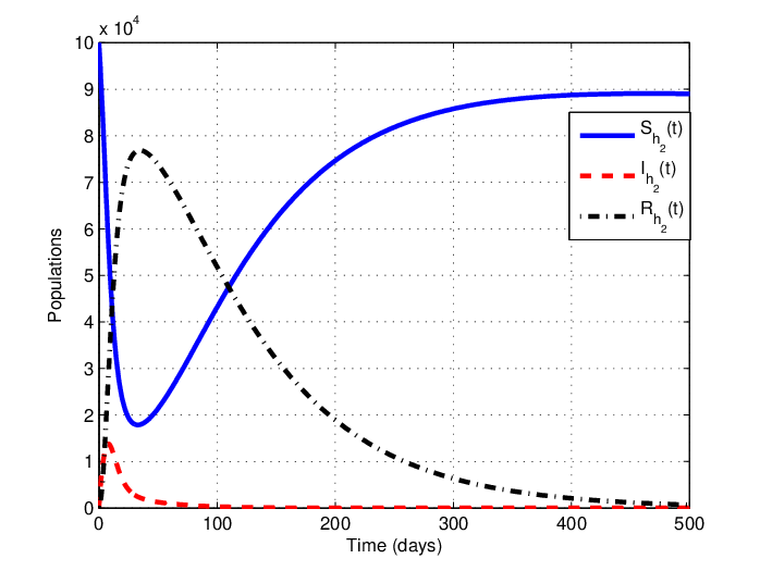
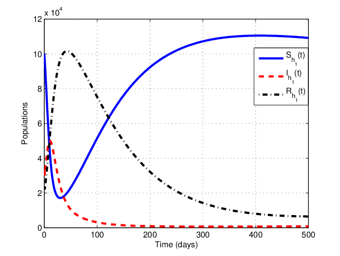
The strongly–coupling scenario is illustrated in Figure 3.3. Here, the disease is spread from patch 1 to patch 2 during the first 100 days and the infection persists in both patches. After 100 days, the disease is eliminated in both patches.

3.2 Local sensitivity analysis of parameters

In this subsection we determine the sensitivity indices of the parameters to the $\mathcal{R}_{0}$ , considering strongly– coupling and data from [27] . The sensitivity indices are computed through the normalized forward sensitivity index [12], which allow us to measure the relative change of the variable $\mathcal{R}_{0}$ when a parameter changes. When the variable is a differentiable function of the parameter, the sensitivity index may be alternatively defined using partial derivatives [12]. If we denote the variable as $u$ which depends on a parameter $p$ , the sensitivity index is defined by

\Gamma_{p}^{u}\doteq\frac{\partial u}{\partial p}\frac{p}{u}.

(3.6)

Given the explicit formula for $\mathcal{R}_{0}$ in (3.5), we determine an analytical expression for the sensitivity indices of $\mathcal{R}_{0}$ with respect to each parameter that comprise it. In Table 3.2 we show the values of the sensitivity indices, where P1 and P2 mean patch 1 and patch 2, respectively.

Table 3.2: Sensitivity indices to the

\mathcal{R}_{0}

with respect to parameters.

Parameter	Index P1	Index P2	Parameter	Index P1	Index P2
$\Lambda_{h_{i}}$	-0.033	-0.4	$\lambda_{11}$	0.00012	0.0086
$\omega_{i}$	0	0	$\lambda_{12}$	0.0042	0.0042
$\beta_{h_{i}}$	0.01	0.50	$\lambda_{22}$	0.0030	0.0030
$\beta_{v_{i}}$	0.09	0.49	$\lambda_{21}$	0.3887	0.3887
$\epsilon_{i}$	0.09	0.90	$q_{1i}$	-0.003	-0.0014
$\mu_{h_{i}}$	0.012	-0.49	$q_{2i}$	-0.1164	-0.00058
$\mu_{v_{i}}$	-0.011	-0.012	$\xi_{1i}$	-0.3488	-0.1405
$\rho_{i}$	-0.0053	-0.0082	$\xi_{2i}$	0.0034	0.0045
$\delta_{i}$	-0.0033	-0.0027	$\theta_{1i}$	-0.54	-0.65
$\Lambda_{v_{i}}$	0.0133	0.50	$\theta_{2i}$	-0.45	-0.98

From Table 3.2, in both rural (patch 1) and urban (patch 2) areas, $\mathcal{R}_{0}$ is more sensitive to the parameters corresponding to recovery rate due to the drug $\theta_{1i}$ with $i=1,2$ and death rate due to the insecticides $\theta_{2i}$ with $i=1,2$ . An interpretation of these indices is given as follows: in RA, given that $\Gamma_{\theta_{11}}=-0.54$ , increasing (or decreasing) $\theta_{11}$ in 10% implies that $\mathcal{R}_{0}$ decreases (or increases) in 5.4%. An analogous reasoning can be made for the others sensitivity indices. The information provided by the sensitivity indices to the $\mathcal{R}_{0}$ , will be used in the next section, in which we will propose some control strategies for the malaria disease.

4 Optimal control problem

In this section an optimal control problem applied to the model (3.1) is formulated. Here, we are going to consider that the parameters corresponding to recovery rate due to the drug and death rate due to the insecticides $\theta_{ij}$ with $i,j=1,2$ will be the controls, therefore they will be functions depending on time. The first objective will be to minimize a performance index or cost function by the use of drugs and insecticides. For this purpose, we assume that $\theta_{i1}$ with $i=1,2$ and $\theta_{j2}$ with $j=1,2$ are the controls by drugs and insecticides, respectively, which assume values between $0$ and $1$ , where $\theta_{ij}=0$ is assumed if the use of drugs (or insecticides) is ineffective and $\theta_{ij}=1$ if the use of drugs (or insecticides) is completely effective, that is, all individuals recover with medication and all mosquitoes die with insecticides. In this sense, for $i$ and $j$ fixed, the control variable $\theta_{ij}(t)$ provides information about amount of drug or insecticides that must be supplied at time $t$ .

The second objective will be to minimize the number of infected humans and infected mosquitoes in each patch. For this purpose, the following performance index or cost function is considered:

J[\bm{\theta}]=\int_{0}^{T}\left[c_{1}(I_{h_{1}}+I_{v_{1}})+c_{2}(I_{h_{2}}+I_{v_{2}})+\frac{1}{2}(d_{1}\theta_{11}^{2}+d_{2}\theta_{21}^{2}+d_{3}\theta_{12}^{2}+d_{4}\theta_{22}^{2})\right]dt,

(4.1)

where $\bm{\theta}=(\theta_{11},\theta_{21},\theta_{12},\theta_{22})$ is the vector of controls, $c_{1}$ and $c_{2}$ represent social costs, which depend on the number of individuals with malaria and the number of mosquitoes with the parasite, and $\frac{1}{2}(d_{1}\theta_{11}^{2}+d_{2}\theta_{21}^{2}+d_{3}\theta_{12}^{2}+d_{4}\theta_{22}^{2})$ defines the absolute costs associated with the control strategies, such as, implementation, ordering, distribution, marketing, among others. For calculation purposes, we will denote to the integrand of the performance index given on (4.1) as

f_{0}(t,\mathbf{X},\bm{\theta})=c_{1}(I_{h_{1}}+I_{v_{1}})+c_{2}(I_{h_{2}}+I_{v_{2}})+\frac{1}{2}(d_{1}\theta_{11}^{2}+d_{2}\theta_{21}^{2}+d_{3}\theta_{12}^{2}+d_{4}\theta_{22}^{2}),

(4.2)

where $\mathbf{X}$ represents the vector of states.

With the above considerations, the following control problem is formulated.

\left\{\begin{array}[]{ll}&\min_{\bm{\theta}\in U}J[\bm{\theta}]=\int\limits_{0}^{T}f_{0}(t.\mathbf{X},\bm{\theta})dt\\ \\ &\dot{S_{h_{i}}}=\Lambda_{h_{i}}+\omega_{i}R_{h_{i}}-S_{h_{i}}\sum_{j=1}^{2}\lambda_{ij}\beta_{hj}\epsilon_{j}\frac{I_{v_{j}}}{N_{h_{j}}}-\mu_{h_{i}}S_{h_{i}}\\ \\ &\dot{I_{h_{i}}}=\sum_{j=1}^{2}\lambda_{ij}\beta_{hj}\epsilon_{j}\frac{I_{v_{j}}}{N_{h_{j}}}-\xi_{1i}\theta_{1i}(t)(1-q_{1i})I_{h_{i}}-(\delta_{i}+\rho_{i}+\mu_{h_{i}})I_{h_{i}}\\ \\ &\dot{R_{h_{i}}}=\xi_{1i}\theta_{1i}(t)(1-q_{1i})I_{h_{i}}+\delta_{i}I_{h_{i}}-(\omega_{i}+\mu_{h_{i}})R_{h_{i}}\\ \\ &\dot{S_{v_{i}}}=\Lambda_{v_{i}}-S_{v_{i}}\sum_{j=1}^{2}\lambda_{ji}\beta_{vj}\epsilon_{j}\frac{I_{h_{j}}}{N_{h_{j}}}-\xi_{2i}\theta_{2i}(t)(1-q_{2i})-\mu_{v_{i}}S_{v_{i}}\\ \\ &\dot{I_{v_{i}}}=S_{v_{i}}\sum_{j=1}^{2}\lambda_{ji}\beta_{vj}\epsilon_{j}\frac{I_{h_{j}}}{N_{h_{j}}}-\xi_{2i}\theta_{2i}(t)(1-q_{2i})-\mu_{v_{i}}I_{v_{i}},\quad\text{for}\quad i=1,2\\ \\ &\mathbf{X}(0)=(\mathbf{N}_{h_{1}}(0),\mathbf{N}_{v_{1}}(0),\mathbf{N}_{h_{2}}(0),\mathbf{N}_{v_{2}}(0))=\mathbf{X}_{0}\\ \\ &\mathbf{X}(T)=(\mathbf{N}_{h_{1}}(T),\mathbf{N}_{v_{1}}(T),\mathbf{N}_{h_{2}}(T),\mathbf{N}_{v_{2}}(T))=\mathbf{X}_{1}.\end{array}\right.

(4.3)

In above the formulation, we assume an initial time $t_{0}=0$ , a final time $T$ fixed which represents the implementation time of the control strategies, free dynamic variables $\mathbf{X}_{1}$ in the final time, and the initial condition $\mathbf{X}_{0}$ being a non–trivial equilibrium of the system (3.1). Additionally, we assume that the controls are in a set of admissible controls $\mathcal{U}$ which contains to all Lebesgue measurables functions with values in the interval $[0,1]$ and $t\in[0,T]$ .

4.1 Existence of an optimal control

In this section, we use the classic existence theorem proposed by Lenhart and Workman [21] to prove the existence of an optimal control $\bm{\theta}^{*}$ for the formulation (4.3). Let $U=[0,1]^{4}$ the set where $\bm{\theta}$ assumes its values (set of controls), and $f(t,\mathbf{X},\bm{\theta})$ the state equations of the right side of (4.3). To guarantee the existence of optimal controls, hypotheses (H1) to (H5) from [21] must be verified, that is,

(H1)
- (a)
  
  $|f(t,\mathbf{0},\mathbf{0})|\leq C$
- (b)
  
  $|f_{\mathbf{X}}(t,\mathbf{X},\bm{\theta})|\leq C(1+|\bm{\theta}|)$
- (c)
  
  $|f_{\bm{\theta}}(t,\mathbf{X},\bm{\theta})|\leq C$ .
(H2)

The set of controls $U$ is convex.
(H3)

$f(t,\mathbf{X},\bm{\theta})=\alpha(t,\mathbf{X})+\beta(t,\mathbf{X})\bm{\theta}$ .
(H4)

The integrand of the performance index $f_{0}(t,\mathbf{X},\bm{\theta})$ defined in (4.2) is convex for $\bm{\theta}\in U$ .
(H5)

$f_{0}(t,\mathbf{X},\bm{\theta})\geq c_{1}|\bm{\theta}|^{b}-c_{2}$ with $c_{1}>0$ and $b>1$ .

We will proof the hypothesis (H1)(a) and (H5), since the others are obvious. For this purpose, the following results are enunciated and proved.

Lema 4.1.

Let

\frac{\xi}{2}=\{\max{\xi_{11}^{2}(1-q_{11})^{2},\xi_{12}^{2}(1-q_{12})^{2},\xi_{21}^{2}(1-q_{21})^{2},\xi_{22}^{2}(1-q_{22})^{2}}\}.

(4.4)

Then

|f_{\bm{\theta}}(t,\mathbf{X},\bm{\theta})|\leq\sqrt{\xi\left[\left(\frac{\Lambda_{H}}{\mu_{H}}\right)^{2}+\left(\frac{\Lambda_{V}}{\mu_{V}}\right)^{2}\right]},

(4.5)

where $\Lambda_{H}$ , $\Lambda_{V}$ , $\mu_{H}$ and $\mu_{V}$ are defined on (3.2), and $f_{\bm{\theta}}(t,\mathbf{X},\bm{\theta})$ is the matrix obtained by differentiating of the state equations of the right side of the system (4.3) with respect to $\bm{\theta}$ , whic is given by

f_{\bm{\theta}}(t,\mathbf{X},\bm{\theta})=\left(\begin{array}[]{cccc}0&0&0&0\\ -\xi_{11}(1-q_{11})I_{h_{1}}&0&0&0\\ \xi_{11}(1-q_{11})I_{h_{1}}&0&0&0\\ 0&-\xi_{21}(1-q_{11})S_{v_{1}}&0&0\\ 0&-\xi_{21}(1-q_{11})S_{v_{1}}&0&0\\ 0&0&0&0\\ 0&0&-\xi_{12}(1-q_{12})I_{h_{2}}&0\\ 0&0&\xi_{12}(1-q_{12})I_{h_{2}}&0\\ 0&0&0&-\xi_{22}(1-q_{22})S_{v_{2}}\\ 0&0&0&-\xi_{22}(1-q_{22})I_{v_{2}}\end{array}\right).

(4.6)

Proof.

Computing the Euclidean norm of matrix (4.6), we obtain

\begin{array}[]{ll}|f_{\bm{\theta}}(t,\mathbf{X},\bm{\theta})|&\left(2\xi_{11}^{2}(1-q_{11})^{2}I_{h_{1}}^{2}+\xi_{21}^{2}(1-q_{21})^{2}(S_{v_{1}}^{2}+I_{v_{1}}^{2})+2\xi_{12}^{2}(1-q_{12})^{2}I_{h_{2}}^{2}+\xi_{22}^{2}(1-q_{22}^{2})(S_{v_{2}}^{2}+I_{v_{2}}^{2})\right)^{1/2}\\ \\ &\leq\left(2[\xi_{11}^{2}(1-q_{11})^{2}+\xi_{12}^{2}(1-q-{12})^{2}]\left(\frac{\Lambda_{H}}{\mu_{H}}\right)^{2}+2[\xi_{21}^{2}(1-q_{21})^{2}+\xi_{22}^{2}(1-q_{22})^{2}]\left(\frac{\Lambda_{V}}{\mu_{V}}\right)^{2}\right)^{1/2}\\ \\ &\leq\left(\xi\left[\left(\frac{\Lambda_{H}}{\mu_{H}}\right)^{2}+\left(\frac{\Lambda_{V}}{\mu_{V}}\right)^{2}\right]\right)=|f_{\bm{\theta}}(t,X,\bm{\theta})|.\end{array}

∎

Lema 4.2.

The integrand of the performance index satisfies

f_{0}(t,\mathbf{X},\bm{\theta})\geq\frac{1}{2}\min{\{d_{1},d_{2},d_{3},d_{4}\}}(\theta_{11}^{2}+\theta_{21}^{2}+\theta_{12}^{2}+\theta_{22}^{2}).

Proof.

\begin{array}[]{ll}f_{0}(t,\mathbf{X},\bm{\theta})&=c_{1}(I_{h_{1}}+I_{v_{1}})+c_{2}(I_{h_{2}}+I_{v_{2}})+\frac{1}{2}(\theta_{11}^{2}+\theta_{21}^{2}+\theta_{12}^{2}+\theta_{22}^{2})\\ \\ &\geq\frac{1}{2}(\theta_{11}^{2}+\theta_{21}^{2}+\theta_{12}^{2}+\theta_{22}^{2})\\ \\ &\geq\frac{1}{2}\min{\{d_{1},d_{2},d_{3},d_{4}\}}(\theta_{11}^{2}+\theta_{21}^{2}+\theta_{12}^{2}+\theta_{22}^{2}).\end{array}

(4.7)

∎

Remark 4.3.

Hypothesis (H5) is fullfied by taking $b=2$ , $c_{2}=0$ and $c_{1}=1/2\min{\{d_{1},d_{2},d_{3},d_{4}\}}$ in the last expression of (4.7).

4.2 Deduction of an optimal solution

In this section, the Pontryaguin Principle for bounded controls [21] is used to compute the optimal controls of the problem (4.3). First, let us observe that the Hamiltonian associated to (4.3), is given by

\begin{array}[]{ll}&H(t,\mathbf{X}(t),\bm{\theta}(t),\mathbf{Z}(t))=f_{0}(t,\mathbf{X},\bm{\theta})+\mathbf{Z}\cdot f(t,\mathbf{X},\bm{\theta})=\\ \\ &c_{1}I_{h_{1}}+c_{1}I_{v_{1}}+c_{2}I_{h_{2}}+c_{2}I_{v_{2}}+\frac{1}{2}\left[d_{1}\theta_{11}^{2}+d_{2}\theta_{21}^{2}+d_{3}\theta_{12}^{2}+d_{4}\theta_{22}^{2}\right]\\ \\ +&z_{1}\left[\Lambda_{h_{1}}+\omega_{1}R_{h_{1}}-\left[\lambda_{11}\beta_{h_{1}}\epsilon_{1}\frac{I_{v_{1}}}{N_{h_{1}}}+\lambda_{12}\beta_{h_{2}}\epsilon_{2}\frac{I_{v_{2}}}{N_{h_{2}}}\right]S_{h_{1}}-\mu_{h_{1}}S_{h_{1}}\right]\\ \\ +&z_{2}\left[\left[\lambda_{11}\beta_{h_{1}}\epsilon_{1}\frac{I_{v_{1}}}{N_{h_{1}}}+\lambda_{12}\beta_{h_{2}}\epsilon_{2}\frac{I_{v_{2}}}{N_{h_{2}}}\right]S_{h_{1}}-\xi_{11}\theta_{11}(t)(1-q_{11})I_{h_{1}}-(\delta_{1}+\rho_{1}+\mu_{h_{1}})I_{h_{1}}\right]\\ \\ +&z_{3}\left[\xi_{11}\theta_{11}(t)(1-q_{11})I_{h_{1}}+\delta_{1}I_{h_{1}}-(\omega_{1}+\mu_{h_{1}})R_{h_{1}}\right]\\ \\ +&z_{4}\left[\Lambda_{v_{1}}-\left[\lambda_{11}\beta_{v_{1}}\epsilon_{1}\frac{I_{h_{1}}}{N_{h_{1}}}+\lambda_{21}\beta_{v_{2}}\epsilon_{2}\frac{I_{h_{2}}}{N_{h_{2}}}\right]S_{v_{1}}-\xi_{21}\theta_{21}(t)(1-q_{21})S_{v_{1}}-\mu_{v_{1}}S_{v_{1}}\right]\\ \\ +&z_{5}\left[\left[\lambda_{11}\beta_{v_{1}}\epsilon_{1}\frac{I_{h_{1}}}{N_{h_{1}}}+\lambda_{21}\beta_{v_{2}}\epsilon_{2}\frac{I_{h_{2}}}{N_{h_{2}}}\right]S_{v_{1}}-\xi_{21}\theta_{21}(t)(1-q_{21})I_{v_{1}}-\mu_{v_{1}}I_{v_{1}}\right]\\ \\ +&z_{6}\left[\Lambda_{h_{2}}+\omega_{2}R_{h_{2}}-\left[\lambda_{22}\beta_{h_{2}}\epsilon_{2}\frac{I_{v_{2}}}{N_{h_{2}}}+\lambda_{21}\beta_{h_{1}}\epsilon_{1}\frac{I_{v_{1}}}{N_{h_{1}}}\right]S_{h_{2}}-\mu_{h_{2}}S_{h_{2}}\right]\\ \\ +&z_{7}\left[\left[\lambda_{22}\beta_{h_{2}}\epsilon_{2}\frac{I_{v_{2}}}{N_{h_{2}}}+\lambda_{21}\beta_{h_{1}}\epsilon_{1}\frac{I_{v_{1}}}{N_{h_{1}}}\right]S_{h_{2}}-\xi_{12}\theta_{12}(t)(1-q_{12})I_{h_{2}}-(\delta_{2}+\rho_{2}+\mu_{h_{2}})I_{h_{2}}\right]\\ \\ +&z_{8}\left[\xi_{12}\theta_{12}(t)(1-q_{12})I_{h_{2}}+\delta_{2}I_{h_{2}}-(\omega_{2}+\mu_{h_{2}})R_{h_{2}}\right]\\ \\ +&z_{9}\left[\Lambda_{v_{2}}-\left[\lambda_{22}\beta_{v_{2}}\epsilon_{2}\frac{I_{h_{2}}}{N_{h_{2}}}+\lambda_{12}\beta_{v_{1}}\epsilon_{1}\frac{I_{h_{1}}}{N_{h_{1}}}\right]S_{v_{2}}-\xi_{22}\theta_{22}(t)(1-q_{22})S_{v_{2}}-\mu_{v_{2}}S_{v_{2}}\right]\\ \\ +&z_{10}\left[\left[\lambda_{22}\beta_{v_{2}}\epsilon_{2}\frac{I_{h_{2}}}{N_{h_{2}}}+\lambda_{12}\beta_{v_{1}}\epsilon_{1}\frac{I_{h_{1}}}{N_{h_{1}}}\right]S_{v_{2}}-\xi_{22}\theta_{22}(t)(1-q_{22})I_{v_{2}}-\mu_{v_{2}}I_{v_{2}}\right],\end{array}

(4.8)

where $\mathbf{Z}=(z_{1},z_{2},...,z_{10})$ is the vector of adjoint variables which determine the adjoint system. The adjoint system and the state equations of (4.3) define the optimal system. The main result of this section is summarized in the following theorem.

Theorem 4.4.

There are an optimal solution $\mathbf{X}^{*}(t)$ that minimize $J$ in $[0,T]$ , and an adjoint vector of adjoint functions $\mathbf{Z}$ such that

\left\{\begin{array}[]{ll}&\dot{z_{1}}=\mu_{h_{1}}z_{1}+\lambda_{12}\beta_{h_{2}}\epsilon_{2}\frac{I_{v_{2}}}{N_{h_{2}}}(z_{1}-z_{2})+\lambda_{11}\beta_{h_{1}}\epsilon_{1}I_{v_{1}}\frac{N_{h_{1}}-S_{h_{1}}}{N_{h_{1}}^{2}}(z_{1}-z_{2})\\ &+\lambda_{11}\beta_{v_{1}}\epsilon_{1}\frac{I_{h_{1}}S_{v_{1}}}{N_{h_{1}}^{2}}(z_{5}-z_{4})+\lambda_{21}\beta_{h_{1}}\epsilon_{1}\frac{I_{v_{1}}S_{h_{2}}}{N_{h_{1}}^{2}}(z_{7}-z_{6})+\lambda_{12}\beta_{v_{1}}\epsilon_{1}\frac{I_{h_{1}}S_{v_{2}}}{N_{h_{1}}^{2}}(z_{10}-z_{9})\\ \\ &\dot{z_{2}}=-c_{1}-[\xi_{11}\theta_{11}(1-q_{11})+\delta_{1}]z_{3}+\left[\delta_{1}+\rho_{1}+\mu_{h_{1}}-\xi_{11}\theta_{11}(1-q_{11})\right]z_{2}\\ &+\lambda_{11}\beta_{h_{1}}\epsilon_{1}\frac{I_{v_{1}}S_{h_{1}}}{N_{h_{1}}^{2}}(z_{2}-z_{1})\lambda_{11}\beta_{v_{1}}\epsilon_{1}S_{v_{1}}\frac{(N_{h_{1}}-I_{h_{1}})}{N_{h_{1}}^{2}}(z_{4}-z_{5})+\lambda_{21}\beta_{h_{1}}\epsilon_{1}\frac{I_{v_{1}}S_{h_{2}}}{N_{h_{1}}^{2}}(z_{7}-z_{6})\\ &+\lambda_{12}\beta_{v_{1}}\epsilon_{1}S_{v_{2}}\frac{N_{h_{1}}-I_{h_{1}}}{N_{h_{1}}^{2}}(z_{9}-z_{10})\\ \\ &\dot{z_{3}}=-\omega_{1}z_{1}+(\omega_{1}+\mu_{h_{1}})z_{3}+\lambda_{11}\beta_{h_{1}}\epsilon_{1}\frac{I_{v_{1}}S_{h_{1}}}{N_{h_{1}^{2}}}(z_{2}-z_{1})\\ &+\lambda_{11}\beta_{v_{1}}\epsilon_{1}\frac{I_{h_{1}}S_{v_{1}}}{N_{h_{1}}^{2}}(z_{5}-z_{4})+\lambda_{21}\beta_{h_{1}}\epsilon_{1}\frac{I_{v_{1}}S_{h_{2}}}{N_{h_{1}}^{2}}(z_{7}-z_{6})+\lambda_{12}\beta_{v_{1}}\epsilon_{1}\frac{I_{h_{1}}S_{v_{2}}}{N_{h_{1}}^{2}}(z_{10}-z_{9})\\ \\ &\dot{z_{4}}=[\xi_{21}\theta_{21}(1-q_{21})+\mu_{v_{1}}]z_{4}+\left[\lambda_{11}\beta_{v_{1}}\epsilon_{1}\frac{I_{h_{1}}}{N_{h_{1}}}+\lambda_{21}\beta_{v_{2}}\epsilon_{2}\frac{I_{h_{2}}}{N_{h_{2}}}\right](z_{4}-z_{5})\\ \\ \\ &\dot{z_{5}}=-c_{1}+[\xi_{21}\theta_{21}(1-q_{21})+\mu_{v_{1}}]z_{5}+\lambda_{11}\beta_{h_{1}}\epsilon_{1}\frac{S_{h_{1}}}{N_{h_{1}}}(z_{1}-z_{2})+\lambda_{21}\beta_{h_{1}}\epsilon_{1}\frac{S_{h_{2}}}{N_{h_{1}}}(z_{6}-z_{7})\\ \\ &\dot{z_{6}}=-\mu_{h_{2}}z_{6}+\lambda_{12}\beta_{h_{2}}\epsilon_{2}\frac{I_{v_{2}}S_{h_{1}}}{N_{h_{2}}^{2}}(z_{2}-z_{1})+\lambda_{21}\beta_{v_{2}}\epsilon_{2}\frac{I_{h_{2}}S_{v_{1}}}{N_{h_{2}}^{2}}(z_{5}-z_{4})\\ &+\lambda_{22}\beta_{h_{2}}\epsilon_{2}I_{v_{2}}\frac{N_{h_{2}}-S_{h_{2}}}{N_{h_{2}}^{2}}(z_{6}-z_{7})+\lambda_{21}\beta_{h_{1}}\epsilon_{1}\frac{I_{v_{1}}}{N_{h_{1}}}(z_{6}-z_{7})+\lambda_{22}\beta_{v_{2}}\epsilon_{2}\frac{I_{h_{2}}S_{v_{2}}}{N_{h_{2}}^{2}}(z_{9}-z_{10})\\ \\ &\dot{z_{7}}=-c_{1}-(\xi_{12}\theta_{12}(1-q_{12})+\delta_{2})z_{8}+[\xi_{12}\theta_{12}(1-q_{12})+\delta_{2}+\rho_{2}+\mu_{h_{2}}]z_{7}\\ &+\lambda_{12}\beta_{h_{2}}\epsilon_{2}\frac{I_{v_{2}}S_{h_{1}}}{N_{h_{2}}^{2}}(z_{2}-z_{1})+\lambda_{21}\beta_{v_{2}}\epsilon_{2}S_{v_{1}}\frac{(N_{h_{2}}-I_{h_{2}})}{N_{h_{2}}^{2}}(z_{5}-z_{4})\\ &+\lambda_{22}\beta_{h_{2}}\epsilon_{2}\frac{I_{v_{2}}S_{h_{2}}}{N_{h_{2}}^{2}}(z_{7}-z_{6})+\lambda_{22}\beta_{v_{2}}\epsilon_{2}S_{v_{2}}\frac{N_{h_{2}}-I_{h_{2}}}{N_{h_{2}}^{2}}(z_{9}-z_{10})\\ \\ &\dot{z_{8}}=-\omega_{2}z_{6}+(\omega_{2}+\mu_{h_{2}})z_{8}+\lambda_{12}\beta_{h_{2}}\epsilon_{2}\frac{I_{v_{2}}S_{h_{1}}}{N_{h_{2}}^{2}}(z_{2}-z_{1})+\\ &\lambda_{21}\beta_{v_{2}}\epsilon_{2}\frac{I_{h_{2}}S_{v_{1}}}{N_{h_{2}}^{2}}(z_{5}-z_{4})+\lambda_{22}\beta_{h_{2}}\epsilon_{2}\frac{I_{v_{2}}S_{h_{2}}}{N_{h_{2}}^{2}}(z_{7}-z_{6})+\lambda_{22}\beta_{v_{2}}\epsilon_{2}\frac{I_{h_{2}}S_{v_{2}}}{N_{h_{2}}^{2}}(z_{10}-z_{9})\\ \\ &\dot{z_{9}}=[\xi_{22}\theta_{22}(1-q_{22})+\mu_{v_{2}}]z_{9}+\left[\lambda_{22}\beta_{v_{2}}\epsilon_{2}\frac{I_{h_{2}}}{N_{h_{2}}}+\lambda_{12}\beta_{v_{1}}\epsilon_{1}\frac{I_{h_{1}}}{N_{h_{1}}}\right](z_{9}-z_{10})\\ \\ \\ &\dot{z_{10}}=-c_{2}+[\xi_{22}\theta_{22}(1-q_{22})+\mu_{v_{2}}]z_{10}+\lambda_{22}\beta_{h_{2}}\epsilon_{2}\frac{S_{h_{2}}}{N_{h_{2}}}(z_{6}-z_{7})+\lambda_{12}\beta_{h_{2}}\epsilon_{2}\frac{S_{h_{1}}}{N_{h_{2}}}(z_{1}-z_{2}),\\ \\ \end{array}\right.

(4.9)

with transversality condition $\mathbf{Z}(t)=\mathbf{0}$ and the following characterization of the controls

\left\{\begin{array}[]{lll}\theta_{11}^{*}=&\min\left\{\max\left\{0,\frac{\xi_{11}(1-q_{11})I_{h_{1}}(z_{2}-z_{3})}{d_{1}}\right\},1\right\}\\ \\ \theta_{21}^{*}=&\min\left\{\max\left\{0,\frac{\xi_{21}(1-q_{21})(S_{v_{1}}z_{4}+I_{v_{1}}z_{5})}{d_{2}}\right\},1\right\}\\ \\ \theta_{12}^{*}=&\min\left\{\max\left\{0,\frac{\xi_{12}(1-q_{12})I_{h_{2}}(z_{7}-z_{8})}{d_{3}}\right\},1\right\}\\ \\ \theta_{22}^{*}=&\min\left\{\max\left\{0,\frac{\xi_{22}(1-q_{22})(S_{v_{2}}z_{9}+I_{v_{2}}z_{10})}{d_{4}}\right\},1\right\}.\end{array}\right.

(4.10)

Proof.

The Pontryaguin Principle guarantees the existence of the vector of adjoint variables $\mathbf{Z}$ whose components satisfy

$\displaystyle\dot{z_{i}}=\frac{dz_{i}}{dt}$	$\displaystyle=$	$\displaystyle-\frac{\partial H}{\partial x_{i}}$
$\displaystyle z_{i}(T)$	$\displaystyle=$	$\displaystyle 0,\quad i=1,2,...,10$
$\displaystyle H(t,\mathbf{X},\bm{\theta},\mathbf{Z})$	$\displaystyle=$	$\displaystyle\max_{\bm{\theta}\in U}H(t,\mathbf{X},\bm{\theta},\mathbf{Z}).$	(4.11)

Thus, the derivatives of the adjoint variables are

$\displaystyle\dot{z_{1}}$	$\displaystyle=-\frac{\partial H}{\partial S_{h_{1}}},\quad z_{1}(T)=0$	$\displaystyle\dot{z_{6}}$	$\displaystyle=-\frac{\partial H}{\partial S_{h_{2}}},\quad z_{6}(T)=0$
$\displaystyle\dot{z_{2}}$	$\displaystyle=-\frac{\partial H}{\partial I_{h_{1}}},\quad z_{2}(T)=0$	$\displaystyle\dot{z_{7}}$	$\displaystyle=-\frac{\partial H}{\partial I_{h_{2}}},\quad z_{7}(T)=0$
$\displaystyle\dot{z_{3}}$	$\displaystyle=-\frac{\partial H}{\partial R_{h_{1}}},\quad z_{3}(T)=0$	$\displaystyle\dot{z_{8}}$	$\displaystyle=-\frac{\partial H}{\partial R_{h_{2}}},\quad z_{8}(T)=0$
$\displaystyle\dot{z_{4}}$	$\displaystyle=-\frac{\partial H}{\partial S_{v_{1}}},\quad z_{4}(T)=0$	$\displaystyle\dot{z_{9}}$	$\displaystyle=-\frac{\partial H}{\partial S_{v_{2}}},\quad z_{9}(T)=0.$
$\displaystyle\dot{z_{5}}$	$\displaystyle=-\frac{\partial H}{\partial I_{v_{1}}},\quad z_{5}(T)=0$	$\displaystyle\dot{z_{10}}$	$\displaystyle=-\frac{\partial H}{\partial I_{v_{2}}},\quad z_{10}(T)=0.$

Replacing the derivatives of $H$ with respect to the state equations in above equalities, we obtain the system (4.9). Additionally, the optimality conditions for the Hamiltonian are given by

\frac{\partial H}{\partial\theta_{11}^{*}}=\frac{\partial H}{\partial\theta_{12}^{*}}=\frac{\partial H}{\partial\theta_{21}^{*}}=\frac{\partial H}{\partial\theta_{22}^{*}}=0,

from where

$\displaystyle\theta_{11}^{*}$	$\displaystyle=$	$\displaystyle\frac{\xi_{11}(1-q_{11})I_{h_{1}}(z_{2}-z_{3})}{d_{1}}$
$\displaystyle\theta_{21}^{*}$	$\displaystyle=$	$\displaystyle\frac{\xi_{21}(1-q_{21})(S_{v_{1}}z_{4}+I_{v_{1}}z_{5})}{d_{2}}$
$\displaystyle\theta_{12}^{*}$	$\displaystyle=$	$\displaystyle\frac{\xi_{12}(1-q_{12})I_{h_{2}}(z_{7}-z_{8})}{d_{3}}$
$\displaystyle\theta_{22}^{*}$	$\displaystyle=$	$\displaystyle\frac{\xi_{22}(1-q_{22})(S_{v_{2}}z_{9}+I_{v_{2}}z_{10})}{d_{4}}.$

In consequence, $\theta_{11}^{*}$ satisfies

\theta_{11}^{*}=\left\{\begin{array}[]{ccc}1&if&\frac{\xi_{11}(1-q_{11})I_{h_{1}}(z_{2}-z_{3})}{d_{1}}>0\\ \frac{\xi_{11}(1-q_{11})I_{h_{1}}(z_{2}-z_{3})}{d_{1}}&if&0\leq\frac{\xi_{11}(1-q_{11})I_{h_{1}}(z_{2}-z_{3})}{d_{1}}\leq 1\\ 0&if&\frac{\xi_{11}(1-q_{11})I_{h_{1}}(z_{2}-z_{3})}{d_{1}}<0,\end{array}\right.

or equivalently

\theta_{11}^{*}=\min\left\{\max\left\{0,\frac{\xi_{11}(1-q_{11})I_{h_{1}}(z_{2}-z_{3})}{d_{1}}\right\},1\right\}.

(4.12)

Using a similar reasoning for $\theta_{21}^{*}$ , $\theta_{12}^{*}$ and $\theta_{22}^{*}$ we obtain the characterization (4.10) which completes the proof. ∎

5 Numerical experiments

In this section we present some numerical simulations associated with the implementation of drugs and insecticides as control strategies, as well as their effects on the infected individuals under uncoupled and strongly–coupling scenarios. For the simulations, we use the forward-backward sweep method proposed by Lenhart and Workman [21]. The implementation time of the control strategies will be approximately 10 days, which is the duration of a malaria treatment. The values of the relative weights associated with the control, will be those of Table 7 from [27].

Figure 5.1 shows the behavior of the infected individuals in patches 1 and 2 under uncoupled scenario. Due to in this scenario, the disease only remains in patch 1 and does not spread to patch 2, the density of infected individuals decreases with control in patch 1 and the effects of the controls in patch 2 are not necessary.

In Figure 5.2 we can see the behavior of infected individuals in patches 1 and 2 under strongly–coupling scenario. Here, the infection decreases with control in both patches, but the efforts are greater in patch 1 than in patch 2.

In both cases, uncoupled and strongly–coupling scenario, the effects of the controls are highly effective and fast to eliminate the disease in patch 1, while in patch 2 the elimination depends of the coupling scenario.

6 Discusion

In this work, we model the malaria transmission dynamics, considering three factors that hinder its control: resistance to drugs, resistance to insecticides and population movement. To illustrate the above factors, we divide our work into two mathematical models. (a) A mathematical model in a patch under the hypothesis that the parasites are resistant to the drugs, and the mosquitoes are resistant to the insecticides. In this first model, we make a qualitative analysis of the solutions of the system, which reveal the existence of a forward bifurcation and the global stability of the DFE. From the biological point of view, the existence of a forward bifurcation indicates that the disease can be controlled by keeping the local $\mathcal{R}_{0_{one}}$ below of one. Since the expression for $\mathcal{R}_{0_{one}}$ given on (2.8) depends directly on the resistance acquisition ratios $q_{1}$ and $q_{2}$ , then at lower levels of resistance acquisition, the value of $\mathcal{R}_{0_{one}}$ decreases, which implies that the infection levels decrease. On the other hand, since $\mathcal{R}_{0_{one}}$ depends inversely on the effects of the drugs and insecticides, then an increase in the recovery rate of humans due to drugs and the death of mosquitoes due insecticides, implies a decrease of $\mathcal{R}_{0_{one}}$ and therefore the burden of infection. The numerical experiments for this first model corroborate the theoretical results. Here, we assume that the infected patients are treated with ACT (artemisinin–based combination therapy) and to contrast the fumigation of mosquitoes with deltamethrin and cifluthrin, where the first insecticide is more effective than the second one. With total resistance to the drugs and insecticides ( $q_{1}=q_{2}=1$ ), we verify that the burden of infection persists regardless of the type of drug and insecticide used, while without resistance ( $q_{1}=q_{2}=0$ ), the burden of infection decreases with the use of deltamethrin and is maintained at low levels with the use of cifluthrin. These results are alarms in public health, because despite the pharmaceutical industry is taking care day after day to create new drugs and new insecticides, if the phenomenon of resistance acquisition is not counteracted, the problem of malaria control will be increasingly difficult, and in some cases impossible.

(b) For the model in two patches, we consider the same hypotheses of the model in a single patch, and additionally, movement of populations between two patches. For this case, we determine the global basic reproductive number $\mathcal{R}_{0}$ , and through numerical experiments, we illustrate the behavior of the solutions when the infection starts in the patch 1 (rural areas of Tumaco [27]), and under three coupling scenarios: (1) uncoupled scenario. When there is no movement between patches, the infection remains endemic in the patch 1 and does not spread to the patch 2. (2) Weakly–coupling. If the probabilities of visiting between both patches are low, the disease is endemic in the patch 1 and remains at a very low load in the patch 2. (3) Strongly–coupling. If the probabilities of visiting between both patches is high, the disease remains endemic in both patches. These results corroborate the phenomenon of reinfection in areas where malaria has been eradicated and is not endemic, as is the case of urban malaria. Here, a new alarm in public health is created, because if malaria has been completely eradicated in a sector and is not endemic there, the movement of humans (or mosquitoes) from endemic areas can activate the infection alarm again.

Finally, using results of a local sensitivity analysis of parameters to the global $\mathcal{R}_{0}$ , we formulated an optimal control problem by using of drugs and insecticides as control strategies. The results of the theoretical and numerical analysis of the optimal control problem reveal that under uncoupled scenario, the control is effective and necessary in patch 1 but not in patch 2, while under strongly–coupling, greater efforts are required to control the disease in patch 1 than in patch 2.

An open problem through this research is to incorporate prophylaxis as a control strategy for the disease, that is, patient education campaigns both in the use of drugs and in the use of insecticides. In this way, the resistance phenomenon will be mitigated and the control campaigns for the disease will be more effective and less expensive.

References

[1] F. B. Agusto, Malaria drug resistance: The impact of human movement and spatial heterogeneity, Bulletin of Mathematical Biology, 76 (2014), 1607–1641,
[2] D. Aldila, N. Nuraini, E. Soewono and A. Supriatna, Mathematical model of temephos resistance in aedes aegypti mosquito population, in AIP Conference Proceedings, vol. 1589, AIP, 2014, 460–463.
[3] N. Alphey, P. G. Coleman, C. A. Donnelly and L. Alphey, Managing insecticide resistance by mass release of engineered insects, Journal of Economic Entomology, 100 (2014), 1642–1649,
[4] B. Anderson, J. Jackson and M. Sitharam, Descartes’ rule of signs revisited, The American Mathematical Monthly, 105 (1998), 447–451.
[5] S. Aneke, Mathematical modelling of drug resistant malaria parasites and vector populations, Mathematical Methods in the Applied Sciences, 25 (2002), 335–346,
[6] N. Bacaër and C. Sokhna, A reaction-diffusion system modeling the spread of resistance to an antimalarial drug, Mathematical Biosciences and Engineering, 2 (2005), 227–238,
[7] E. Barrios, S. Lee and O. Vasilieva, Assessing the effects of daily commuting in two-patch dengue dynamics: A case study of cali, colombia, Journal of Theoretical Biology, 453 (2018), 14–39,
[8] D. Bichara and A. Iggidr, Multi-patch and multi-group epidemic models: a new framework, Journal of Mathematical Biology, 77 (2018), 107–134.
[9] P. B. Bloland, Drug resistance in malaria, Technical report, Geneva: World Health Organization, 2001.
[10] W. Bock and Y. Jayathunga, Optimal control and basic reproduction numbers for a compartmental spatial multipatch dengue model, Mathematical Methods in the Applied Sciences, 41 (2018), 3231–3245.
[11] C. Castillo-Chavez and B. Song, Dynamical models of tuberculosis and their applications, Mathematical Biosciences and Engineering, 1 (2004), 361–404.
[12] N. Chitnis, J. M. Hyman and J. M. Cushing, Determining important parameters in the spread of malaria through the sensitivity analysis of a mathematical model, Bulletin of Mathematical Biology, 70 (2008), 1272,
[13] E. X. DeJesus and C. Kaufman, Routh–hurwitz criterion in the examination of eigenvalues of a system of nonlinear ordinary differential equations, Physical Review, 35 (1987), 5288.
[14] L. Esteva, A. B. Gumel and C. V. De LeóN, Qualitative study of transmission dynamics of drug-resistant malaria, Mathematical and Computer Modelling, 50 (2009), 611–630,
[15] D. Gao and S. Ruan, A multipatch Malaria model with logistic growth populations, SIAM Journal on Applied Mathematics, 72 (2012), 819–841.
[16] S. A. Gourley, R. Liu and J. Wu, Slowing the evolution of insecticide resistance in mosquitoes: a mathematical model, Proceedings of the Royal Society: mathematical, physical and engineering sciences, 467 (2011), 2127–2148,
[17] C. Guinovart, M. Navia, M. Tanner and P. Alonso, Malaria: burden of disease, Current Molecular Medicine, 6 (2006), 137–140,
[18] J. Hasler, Stochastic and deterministic multipatch epidemic models, ProQuest LLC, Ann Arbor, MI, 2016, Thesis (Ph.D.)–University of Illinois at Urbana-Champaign.
[19] J. Koella and R. Antia, Epidemiological models for the spread of anti–malarial resistance, Malaria Journal, 2 (2003), 3,
[20] S. Lee and C. Castillo-Chavez, The role of residence times in two-patch dengue transmission dynamics and optimal strategies, Journal of Theoretical Biology, 374 (2015), 152–164,
[21] S. Lenhart and J. T. Workman, Optimal control applied to biological models, Crc Press, 2007.
[22] P. Luz, C. Codeco, J. Medlock, C. Struchiner, D. Valle and A. Galvani, Impact of insecticide interventions on the abundance and resistance profile of aedes aegypti, Epidemiology and Infection, 137 (2009), 1203–1215.
[23] A. Mishra and S. Gakkhar, Non-linear dynamics of two-patch model incorporating secondary dengue infection, International Journal of Applied and Computational Mathematics, 4 (2018), Art. 19, 22,
[24] K. Okosun and O. D. Makinde, Modelling the impact of drug resistance in malaria transmission and its optimal control analysis, International Journal of the Physical Sciences, 6 (2011), 6479–6487,
[25] M. Palomino, P. Villaseca, F. Cárdenas, J. Ancca and M. Pinto, Eficacia y residualidad de dos insecticidas piretroides contra triatoma infestans en tres tipos de viviendas: Evaluación de campo en arequipa, perú, Revista Peruana de Medicina Experimental y Salud Pública, 25 (2008), 9–16.
[26] O. Prosper, N. Ruktanonchai and M. Martcheva, Assessing the role of spatial heterogeneity and human movement in malaria dynamics and control, Journal of Theoretical Biology, 303 (2012), 1–14.
[27] J. Romero-Leiton and E. Ibargüen-Mondragón, Stability analysis and optimal control intervention strategies of a malaria mathematical model, Applied Sciences, 21 (2019), 184–218.
[28] S. J. Smith, A. R. Kamara, F. Sahr, M. Samai, A. S. Swaray, D. Menard and M. Warsame, Efficacy of artemisinin-based ombination therapies and prevalence of molecular markers associated with artemisinin, piperaquine and sulfadoxine-pyrimethamine resistance in sierra leone, Actar Tropica, 185 (2018), 363–370.
[29] J. M. Tchuenche, C. Chiyaka, D. Chan, A. Matthews and G. Mayer, A mathematical model for antimalarial drug resistance, Mathematical Medicine and Biology: a Journal of the IMA, 28 (2011), 335–355,
[30] P. Van den Driessche and J. Watmough, Reproduction numbers and sub-threshold endemic equilibria for compartmental models of disease transmission,
[31] D. Wei, X. Luo and Y. Qin, Controlling bifurcation in power system based on lasalle invariant principle, Nonlinear Dynamics, 63 (2011), 323–329,
[32] WHO, Community involvement in rolling back malaria, Geneva: World Health Organization.
[33] J. Zhang, C. Cosner and H. Zhu, Two–patch model for the spread of West Nile virus, Bulletin of Mathematical Biology, 80 (2018), 840–863,