跳到论文正文
W Papers独立论文阅读器 arXiv:2001.11971 论文正文 计算阅读时间 · 0%
引用这篇论文根据当前论文元数据生成,正式投稿前建议核对。


License: arXiv.org perpetual non-exclusive license
arXiv:2001.11971v1 [eess.SY] 31 Jan 2020

Optimal Controller Synthesis and Dynamic Quantizer Switching
for Linear-Quadratic-Gaussian Systems

Dipankar Maity    Panagiotis Tsiotras Thanks:  Thanks: The authors are with the Guggenheim School of Aerospace Engineering, Georgia Institute of Technology, Atlanta, GA, 30332, USA. Email: dmaity@gatech.edu, tsiotras@gatech.edu Thanks: This work has been supported by ARL under DCIST CRA W911NF-17-2-0181 and by ONR award N00014-18-1-2375.
Abstract

In networked control systems, often the sensory signals are quantized before being transmitted to the controller. Consequently, performance is affected by the coarseness of this quantization process. Modern communication technologies allow users to obtain resolution-varying quantized measurements based on the prices paid. In this paper, we consider optimal controller synthesis of a Quantized-Feedback Linear-Quadratic-Gaussian (QF-LQG) system where the measurements are to be quantized before being transmitted to the controller. The system is presented with several choices of quantizers, along with the cost of operating each quantizer. The objective is to jointly select the quantizers and the controller that would maintain an optimal balance between control performance and quantization cost. Under certain assumptions, this problem can be decoupled into two optimization problems: one for optimal controller synthesis and the other for optimal quantizer selection. We show that, similarly to the classical LQG problem, the optimal controller synthesis subproblem is characterized by Riccati equations. On the other hand, the optimal quantizer selection policy is found by solving a certain Markov-Decision-Process (MDP).

I INTRODUCTION

Increasingly, many control systems nowadays consist of multiple sensors, actuators and plants that are spatially distributed. Control of such systems requires uninhibited and reliable exchange of signals among these components over a shared communication network. Often, the underlying communication network suffers from several limitations such as insufficient bandwidth, noisy transmissions, or delays. Although many of these abovementioned limitations can be alleviated with current advancements in communication technologies, at the same time it may be expensive to deploy such a communication infrastructure. Therefore, the performance of such systems no longer depends solely on the controller structure but also on the underlying communication infrastructure and the associated communication cost.

In a typical communication framework, signals are quantized (encoded) before being transmitted through a channel. Upon receiving the transmitted signal, a reconstruction (decoding) is performed to estimate the original signal. Thus, the quality of the quantization dictates the distortion in the reconstructed signal. Higher resolution quantization results in lower distortion. This typically requires a higher number of bits to represent the quantized signal, and hence higher channel bandwidth for transmission. Depending on the criticality of the task, at certain times high-resolution quantization may be required, while other times coarser resolution is sufficient. Therefore, the quantization selection must be adapted optimally over the time horizon to meet the expected quantization-resolution of the transmitted signal with minimal use of the communication resources.

In this work we consider the classical LQG control problem under quantization constraints which can be traced back to [1, 2, 3, 4, 5]. While in most of the prior works, the emphasis has been on the joint design of controller and quantizer, in this paper we take a different approach where instead of designing a quantizer, we formulate a quantizer scheduling problem. In [4] and other related works, the necessity for a time-varying quantizer for stability of linear systems has been studied. Recent works, such as [6], also show the tradeoff between control cost and communication data-rate in the context of infinite-horizon LQG problems. Although LQG optimal control with quantized measurements has been studied for decades, the optimal structure of the controller and quantizer is, however, still unknown. Approximate solutions to the optimal quantizer and controller (for infinite time horizon) synthesis problem have been constructed under restrictive assumptions on the quantization schemes such as lattice quantization [6], entropy coded dithered quantizer for single-input-single-output systems [7, 8] etc.

One may alternatively think of the optimal quantizer design problem as an equivalent problem of selecting the optimal quantizer in the space of quantizers. In this work, instead of designing the quantizers (or equivalently finding the optimal quantizer in the space of quantizers), we ask whether one can find the optimal quantizer(s) from a given set of quantizers. To proceed with this framework, we assume that a control system can choose from a given set of quantizers to quantize its measurements and transmit the quantized signal to the controller. The set of available quantizers is given a priori along with the cost associated with using each quantizer. While the controller aims to minimize the expected quadratic cost, the measurements available to the controller are only the quantized state information. It is worth mentioning here that the observation equations are no longer linear due to the quantization process. The optimization problem under this framework is a bi-variable decision-making problem where one variable is the control strategy and the other one is the scheduling of the quantizers at each time instance.

I-A Prior and Related Work

Some of the earlier works on quantization and control can be traced backed to 1970s [9, 10, 11, 12]. Studies of LQG control under communication constraints with a focus on quantization have been performed in several works such as [1, 2, 3, 5], [13], [14],[15]. For example, [14] considered LQG problems with explicit consideration of the quantization error associated with analog-to-digital implementation. The studies in [13] and [14] showed that the optimal controller does not exhibit the separation principle. It was shown that the optimal controller exhibits a separation principle and that the optimal input-quantizer has to be time-varying with certain specific quantization levels. In [5] the authors provided necessary conditions for the controller to exhibit a separation principle. In [1], the authors provided a quantization scheme that ensures the existence of a separation principle in the optimal controller. In that work, it was proposed to quantize a signal which the authors refer to as “innovations,” rather than quantizing the state. In this work, we will also adhere to the idea of quantizing the “innovations” rather than quantizing the state itself.

Studies on quantization-based control have also dealt with the stability aspects of the system [16, 17, 18, 19, 20]. In [17] and [18], the authors explicitly considered the issues of quantization, coding and delay. The concept of containability was used for studying the stability of linear quantized systems. In [21], three quantization schemes (deadbeat, logarithmic, and chaotic) were proposed to ensure practical stability of a linear system. Optimality of these three quantization schemes was addressed using the notion of symbolic dynamics. Symbolic dynamics based analysis was also used in [12] for extracting state information from quantized measurements. In [22] it was shown that the least dense quantizer that quadratically stabilizes a single input linear system is logarithmic. A logarithmic quantizer with finite quantization level can only achieve practical stabilizability (a relaxed notion of stabilizability). A quantization scheme with time-varying quantization sensitivity was studied in [23] proving asymptotic stability of the system. In [24] the author derived a relationship between the norm of the transition matrix and the number of values taken by the encoder to ensure global asymptotic stability. The work in [25] addressed the problem of finding the smallest data rate above which exponential stability can be ensured. In a more recent work [26], an event-based encoding scheme has been considered.

In the above-mentioned works [1]–[20], the role of quantization has been proven to be crucial. However, for a given control objective, how to select among available quantizers that have an operational cost associated with them has not been addressed, and is the subject of this paper. The problem is similar in spirit to the problem of optimal scheduling of costly sensors for control [27, 28], in the sense that measurements are costly and optimal measurements are chosen to maintain an optimal balance between the control performance and observation cost. It is however different from these works, in the sense that here we study the effects of quantization in producing the measurements sent to the controller whereas such works do not consider the role of quantization.

I-B Contribution

The contributions of this work are:

  • •

    We formulate an LQG optimal control problem with a set of costly quantizers that quantize the measurements. We seek an optimal controller that minimizes the expected quadratic cost and an optimal selection of the quantizers that determine the quality of the measurements arriving at the controller.

  • •

    We show that quantizing the innovations separates the controller synthesis problem from the quantizer selection problem. Although the idea of innovation–quantization is presented in [1], the initial state of the system was needed to be deterministic in that work. Our framework does not require such an assumption.

  • •

    We study the optimal controller structure and show that the controller is of a certainty-equivalence type. The controller gains can be computed offline and the gains do not depend on the parameters of the quantizers.

  • •

    The study of the quantizer-selection reveals that the optimal strategy for the selection of the quantizers can be computed by solving an MDP. Moreover, depending on the information available to the quantizer-selector, the optimal strategy can be computed offline.

I-C Organization

The rest of the paper is organized as follows: in Section II we formally define the problem addressed in this paper; Section III provides the structure for the optimal controller and the quantizer selection scheme; numerical examples illustrating the theory are presented in Section IV. Finally, we conclude the paper with a summary and some remarks in Section VI.

II PROBLEM FORMULATION

Let us consider an LTI discrete-time stochastic system

Xt+1=A​Xt+B​Ut+Wt,\displaystyle X_{t+1}=AX_{t}+BU_{t}+W_{t}, (1)

where for all t∈ℕ0(=ℕ∪{0})t\in\mathbb{N}_{0}~(=\mathbb{N}\cup\{0\}), Xt∈ℝnX_{t}\in\mathbb{R}^{n}, Ut∈ℝmU_{t}\in\mathbb{R}^{m}, AA and BB are matrices of compatible dimensions, and {Wt}t∈ℕ0\{W_{t}\}_{t\in\mathbb{N}_{0}} is an i.i.d noise sequence in ℝn\mathbb{R}^{n} with statistics W0∼𝒩⁡(0,𝒲)W_{0}\sim\mathcal{N}(0,\mathcal{W}). The initial state, X0X_{0}, is also a Gaussian random variable distributed according to 𝒩⁡(μ0,Σ0)\mathcal{N}(\mu_{0},\Sigma_{0}), and independent of the noise WtW_{t} for all t∈ℕ0t\in\mathbb{N}_{0}. For notational convenience, we will write X0=μ0+W−1X_{0}=\mu_{0}+W_{-1} where W−1∼𝒩⁡(0,Σ0)W_{-1}\sim\mathcal{N}(0,\Sigma_{0}). Thus, WkW_{k} and WℓW_{\ell} are independent random variable for all k,ℓ=−1,0,1,…k,\ell=-1,0,1,\ldots and k≠ℓk\neq\ell.

In this work, we address the quantized feedback LQG (QF-LQG) optimal control problem. As shown in Figure 1, we assume that MM quantizers are provided to quantize the state value and transmit the quantized state to the controller. The range of the ii-th quantizer is denoted by 𝒬i={q1i,q2i,…,qℓii}\mathcal{Q}^{i}=\{q_{1}^{i},q_{2}^{i},\ldots,q_{\ell_{i}}^{i}\}. Associated with the ii-th quantizer, let 𝒫i={𝒫1i,𝒫2i,…,𝒫ℓii}\mathcal{P}^{i}=\{\mathcal{P}^{i}_{1},\mathcal{P}^{i}_{2},\ldots,\mathcal{P}^{i}_{\ell_{i}}\} denote a partition in ℝn\mathbb{R}^{n} such that 𝒫ji\mathcal{P}^{i}_{j} gets mapped to qjiq^{i}_{j} for each j∈{1,2,…,ℓi}j\in\{1,2,\ldots,\ell_{i}\}. Specifically, one may think of the ii-th quantizer as a mapping gi:ℝn→𝒬ig_{i}:\mathbb{R}^{n}\to\mathcal{Q}^{i} such that gi​(x)=qjig_{i}(x)=q^{i}_{j} if and only if x∈𝒫jix\in\mathcal{P}^{i}_{j}. Thus, the ii-th quantizer has ℓi\ell_{i} quantization levels. Without loss of generality, we assume that the quantization error covariance decreases from the first quantizer to the MM-th quantizer, i.e., the quantization error covariance is the lowest for the MM-th quantizer and highest for the first quantizer, and so on. Associated with each quantizer, there is an operating cost that must be paid in order to use this quantizer. Let λ⁡(𝒬i)=λi∈ℝ+\lambda(\mathcal{Q}^{i})=\lambda_{i}\in\mathbb{R}_{+} denote the cost associated with the ii-th quantizer11 1 This framework also extends to the scenario where there is no cost in using a quantizer, i.e., λi=0\lambda_{i}=0 for all i=1,…,Mi=1,\ldots,M.. For example, λi=log2⁡ℓi\lambda_{i}=\log_{2}\ell_{i} represents a cost that is proportional to the code-length to encode the output of the quantizer using a simple fixed-length coding scheme. In this work, we do not adhere to any specific structure for λ\lambda. We assume that the values of λi\lambda_{i}’s are given to us a priori. If there is a cost for operating the communication channel, that cost can be also incorporated into λi\lambda_{i}. For example, if every transmission of measurement requires a cost of λc\lambda_{c}, then λi+λc\lambda_{i}+\lambda_{c} represents the joint quantization and communication cost for using ii-th quantizer to transmit a measurement. Designing such costs in order to regulate the use of the quantizers is an equally interesting problem for the service provider, and that will be addressed elsewhere. We will further assume that the communication channel between each quantizer and the controller always transmits the quantized information without any delay or distortion. A discussion on the implications of delay and distortion is provided in Section V.

Set of QuantizersControllerPlantQuantizer Selectorg1​(⋅)g_{1}(\cdot)gM​(⋅)g_{M}(\cdot)g2​(⋅)g_{2}(\cdot)UtU_{t}XtX_{t}θt\theta_{t}Quantized Signal YtY_{t}
Fig. 1: Schematic diagram of the system where the gray block contains the set of quantizers and the desirable quantizer (gig_{i}) is selected by the quantizer selector variable θ\theta.

The objective is to minimize a finite-horizon performance index that takes into account the quantization cost. Contrary to the existing literature on quantization-based LQG [1]-[29], in our case there are two decision-makers instead of one: one (the controller) decides the input ({Ut}t∈ℕ0\{U_{t}\}_{t\in\mathbb{N}_{0}}) to apply to the system, and the other (the quantizer-selector) decides the quality of the measurements (quantized state values) which are transmitted to the controller. That is, the proposed work does not fit with the previous quantization literature that focuses primarily on stability issues or the design of the optimal quantization scheme to maintain performance.

We introduce a new decision variable θti\theta^{i}_{t} for the quantizer-selector in the following way:

θti={1,i​-th quantizer is used at time ​t,0,otherwise.\displaystyle\theta_{t}^{i}=\begin{cases}&1,~~~i\text{-th quantizer is used at time }t,\\ &0,~~~\text{otherwise.}\end{cases}

Let us denote the vector θt≜[θt1,θt2,…,θtM]T∈{0,1}M\theta_{t}\triangleq[\theta_{t}^{1},\theta_{t}^{2},\ldots,\theta_{t}^{M}]^{\mbox{\tiny\sf T}}\in\{0,1\}^{M}, that characterizes the decision of the quantizer-selector at time tt. We enforce the quantizer-selector to select only one quantizer at any time instance, and hence we have ∑i=1Mθti=1\sum_{i=1}^{M}\theta_{t}^{i}=1 for all t∈ℕ0t\in\mathbb{N}_{0}.

The measurement available to the controller at time tt is represented as Yt=∑i=1Mgi​(Xt)​θti=gj​(Xt)​θtjY_{t}=\sum_{i=1}^{M}g_{i}(X_{t})\theta_{t}^{i}=g_{j}(X_{t})\theta^{j}_{t}, if the jj-th quantizer is selected at time tt.22 2 In the following analysis we shall quantize WtW_{t} instead of XtX_{t}. This will help us preserve the separation-principle for the optimal controller as shown in [1]. Let us also introduce the sets 𝒳t≜{X0,X1,…,Xt}\mathcal{X}_{t}\triangleq\{X_{0},X_{1},\ldots,X_{t}\}, 𝒴t≜{Y0,Y1,…,Yt}\mathcal{Y}_{t}\triangleq\{Y_{0},Y_{1},\ldots,Y_{t}\}, 𝒰t≜{U0,U1,…,Ut}\mathcal{U}_{t}\triangleq\{U_{0},U_{1},\ldots,U_{t}\} and Θt≜{θ0,θ1,…,θt}\Theta_{t}\triangleq\{\theta_{0},\theta_{1},\ldots,\theta_{t}\} to be the state history, measurement history, control history and quantization-selection history respectively. For convenience, we will use the notation 𝒰\mathcal{U} for 𝒰T−1\mathcal{U}_{T-1} and, likewise, Θ\Theta for ΘT−1\Theta_{T-1} to denote the history of the entire horizon [0,T][0,T].

The information available to the controller at time tt is ℑtc={𝒴t,𝒰t−1,Θt}=ℑt−1c∪{Yt,Ut−1,θt}\mathfrak{I}_{t}^{c}=\{\mathcal{Y}_{t},\mathcal{U}_{t-1},\Theta_{t}\}=\mathfrak{I}_{t-1}^{c}\cup\{Y_{t},U_{t-1},\theta_{t}\} with ℑ0c={Y0,θ0}\mathfrak{I}_{0}^{c}=\{Y_{0},\theta_{0}\}. It should be noted that ℑtc\mathfrak{I}^{c}_{t} depends on Θt\Theta_{t} through 𝒴t\mathcal{Y}_{t}. In classical optimal LQG control, the information available to the controller is not decided by any active decision maker, unlike the situation here. An admissible control strategy at time tt is a measurable function from the Borel σ\sigma-field generated by ℑtc\mathfrak{I}_{t}^{c} to ℝm\mathbb{R}^{m}. Let us denote such strategies by γtu​(⋅)\gamma^{u}_{t}(\cdot) and the space they belong to by Γtu\Gamma^{u}_{t}. On the other hand, the information available to the quantizer-selector at time tt is ℑtq={𝒳t,𝒴t−1,𝒰t−1,Θt−1}=ℑt−1q∪{Xt,Yt−1,Ut−1,θt−1}\mathfrak{I}_{t}^{q}=\{\mathcal{X}_{t},\mathcal{Y}_{t-1},\mathcal{U}_{t-1},\Theta_{t-1}\}=\mathfrak{I}_{t-1}^{q}\cup\{X_{t},Y_{t-1},U_{t-1},\theta_{t-1}\} with ℑ0q={X0}\mathfrak{I}_{0}^{q}=\{X_{0}\}. The admissible strategies for the selection of the quantizers are measurable functions from the Borel σ\sigma-field generated by ℑtq\mathfrak{I}_{t}^{q} to {0,1}M\{0,1\}^{M}. Let us denote such strategies by γtθ​(⋅)\gamma^{\theta}_{t}(\cdot), and the space they belong to by Γtθ\Gamma^{\theta}_{t}. For brevity, often we will use γtu\gamma^{u}_{t} instead of γtu​(⋅)\gamma^{u}_{t}(\cdot) or γtu​(ℑtc)\gamma^{u}_{t}(\mathfrak{I}_{t}^{c}), and γtθ\gamma^{\theta}_{t} instead of γtθ​(⋅)\gamma^{\theta}_{t}(\cdot) or γtθ​(ℑtq)\gamma^{\theta}_{t}(\mathfrak{I}^{q}_{t}). Let γΘ\gamma^{\Theta} denote the entire sequence {γ0θ,γ1θ,…,γT−1θ}\{\gamma^{\theta}_{0},\gamma^{\theta}_{1},\ldots,\gamma^{\theta}_{T-1}\} and let ΓΘ\Gamma^{\Theta} denote the space where γΘ\gamma^{\Theta} belongs to. Likewise, γ𝒰\gamma^{\mathcal{U}} and Γ𝒰\Gamma^{\mathcal{U}} are defined similarly. The sequence of decision-making within one time instance is then as follows:
⋯→ℑtq​→γtθ​θt→Yt→ℑtc​→γtu​Ut→Xt+1→ℑt+1q→⋯\cdots\to\mathfrak{I}_{t}^{q}\overset{\gamma^{\theta}_{t}}{\rightarrow}\theta_{t}\to Y_{t}\to\mathfrak{I}_{t}^{c}\overset{\gamma^{u}_{t}}{\to}U_{t}\to X_{t+1}\to\mathfrak{I}_{t+1}^{q}\to\cdots.

The cost function to be minimized cooperatively by the controller and the quantizer-selector is a finite horizon quadratic criterion, given as

J⁡(𝒰,Θ)=𝖤⁡[∑t=0T−1(XtT​Q1​Xt+UtT​R​Ut+θtT​Λ)+XTT​Q2​XT],\displaystyle J(\mathcal{U},\Theta)=\mathsf{E}\left[\sum_{t=0}^{T-1}(X_{t}^{\mbox{\tiny\sf T}}Q_{1}X_{t}+U_{t}^{\mbox{\tiny\sf T}}RU_{t}+\theta_{t}^{\mbox{\tiny\sf T}}\Lambda)+X_{T}^{\mbox{\tiny\sf T}}Q_{2}X_{T}\right], (2)

where Λ=[λ1,λ2,…,λM]T\Lambda=[\lambda_{1},\lambda_{2},\ldots,\lambda_{M}]^{\mbox{\tiny\sf T}}, Q1,Q2⪰0,R≻0Q_{1},Q_{2}\succeq 0,R\succ 0, 𝒰=γ𝒰​(ℑc)={γ0u​(ℑ0c),γ1u​(ℑ1c),…,γT−1u​(ℑT−1c)}\mathcal{U}=\gamma^{\mathcal{U}}(\mathfrak{I}^{c})=\{\gamma^{u}_{0}(\mathfrak{I}_{0}^{c}),\gamma^{u}_{1}(\mathfrak{I}_{1}^{c}),\ldots,\gamma_{T-1}^{u}(\mathfrak{I}_{T-1}^{c})\} and Θ=γΘ​(ℑq)={γ0θ​(ℑ0q),γ1θ​(ℑ1q),…,γT−1θ​(ℑT−1q)}\Theta=\gamma^{\Theta}(\mathfrak{I}^{q})=\{\gamma^{\theta}_{0}(\mathfrak{I}_{0}^{q}),\gamma^{\theta}_{1}(\mathfrak{I}_{1}^{q}),\ldots,\gamma_{T-1}^{\theta}(\mathfrak{I}_{T-1}^{q})\}. We seek to find the optimal strategies γ𝒰∗={γ0u∗,γ1u∗,…,γT−1u∗}\gamma^{\mathcal{U}*}=\{\gamma_{0}^{u*},\gamma_{1}^{u*},\ldots,\gamma_{T-1}^{u*}\} and γΘ∗={γ0θ∗,γ1θ∗,…,γT−1θ∗}\gamma^{\Theta*}=\{\gamma^{\theta*}_{0},\gamma^{\theta*}_{1},\ldots,\gamma^{\theta*}_{T-1}\} that minimize (2). To this end, we will also rewrite (2) in terms of γ𝒰\gamma^{\mathcal{U}} and γΘ\gamma^{\Theta} as

J(γ𝒰,γΘ)=𝖤[\displaystyle J(\gamma^{\mathcal{U}},\gamma^{\Theta})=\mathsf{E}\Big[ ∑t=0T−1(XtT​Q1​Xt+UtT​R​Ut+θtT​Λ)+XTT​Q2​XT\displaystyle\sum_{t=0}^{T-1}(X_{t}^{\mbox{\tiny\sf T}}Q_{1}X_{t}+U_{t}^{\mbox{\tiny\sf T}}RU_{t}+\theta_{t}^{\mbox{\tiny\sf T}}\Lambda)+X_{T}^{\mbox{\tiny\sf T}}Q_{2}X_{T}
|Ut=γtu(ℑtc),θt=γtθ(ℑtq)].\displaystyle~~~|~U_{t}=\gamma^{u}_{t}(\mathfrak{I}^{c}_{t}),\theta_{t}=\gamma^{\theta}_{t}(\mathfrak{I}^{q}_{t})\Big]. (3)

We emphasize that ℑtq\mathfrak{I}^{q}_{t} contains the state value XtX_{t} for all tt. Such an information structure will be refereed to as perfect measurement quantizer selection. In Section III-B, we will consider a different information structure for ℑtq\mathfrak{I}^{q}_{t} where XtX_{t} is not present, and ℑtq\mathfrak{I}^{q}_{t} contains the same quantized signals as the controller information. Such information pattern will be referred to as quantized measurement quantizer selection. The perfect measurement quantizer selection leads to a MDP formulation, which is more computationally expensive to solve compared to the quantized measurement quantizer selection scenario which can be solved through linear programming. As will be discussed in detail later, the available information for selecting the quantizers in the quantized measurement case is a subset of the information available for the perfect measurement case. Thus, the perfect measurement scenario results in better performance (i.e., lower cost) than the quantized measurement case, albeit at an expense of higher computation complexity.

III Optimal Control and Quantization Selection

III-A Perfect Measurement Quantizer Selection

In this section we find the optimal γ𝒰∗\gamma^{\mathcal{U}*} and γΘ∗\gamma^{\Theta*} that minimize the cost function (II) amongst all admissible strategies, that is,

(γ𝒰∗,γΘ∗)=arg⁡minγ𝒰∈Γ𝒰,γΘ∈ΓΘJ(γ𝒰,γΘ).\displaystyle(\gamma^{\mathcal{U}*},\gamma^{\Theta*})=\underset{\gamma^{\mathcal{U}}\in\Gamma^{\mathcal{U}},\gamma^{\Theta}\in\Gamma^{\Theta}}{\arg\min}J(\gamma^{\mathcal{U}},\gamma^{\Theta}). (4)

Before proceeding further to solve (4), let us specify the input for the quantization process, since it will play a crucial role in the following analysis. Unlike other quantized feedback based control approaches [13], [14], we will quantize Wt−1W_{t-1} instead of XtX_{t} at time tt. Note that, Wt−1W_{t-1} can be readily computed from the values of Xt,Xt−1,Ut−1X_{t},X_{t-1},U_{t-1} that are included in ℑtq\mathfrak{I}^{q}_{t}. In the existing literature [6, 4] it has been shown that quantizing the state leads to a problem that is intractable, whereas in [1] the utility of noise quantization has been proposed. The schematic for the noise quantization based framework is presented in Figure 2.

Set of QuantizersControllerPlantQuantizer SelectorInnovation extractiong1​(⋅)g_{1}(\cdot)gM​(⋅)g_{M}(\cdot)g2​(⋅)g_{2}(\cdot)UtU_{t}XtX_{t}Wt−1W_{t-1}Quantized Signal w^t−1​(θt)\hat{w}_{t-1}(\theta_{t})θt\theta_{t}
Fig. 2: Schematic diagram of the (perfect measurement quantizer selection) system, where the gray block contains the set of quantizers and the desirable quantizer (gig_{i}) is selected by the quantizer selector variable θ\theta.

Let gi​(Wt−1)∈𝒬ig_{i}(W_{t-1})\in\mathcal{Q}^{i} denote the quantized version of Wt−1W_{t-1} if the ii-th quantizer is selected. Therefore, the quantized information sent to the controller is

Yt=∑i=1Mgi​(Wt−1)​θti\displaystyle Y_{t}=\sum_{i=1}^{M}g_{i}(W_{t-1})\theta^{i}_{t} (5)

Note that YtY_{t} is a random variable taking values in the discrete set ∪i=1M𝒬i\cup_{i=1}^{M}\mathcal{Q}^{i} with 𝖯⁡(Yt=qji)=𝖯⁡(Wt−1∈𝒫ji)\mathsf{P}(Y_{t}=q^{i}_{j})=\mathsf{P}(W_{t-1}\in\mathcal{P}^{i}_{j}). Let us now define w^ti≜𝖤⁡[Wt|gi​(Wt)]\hat{w}_{t}^{i}\triangleq\mathsf{E}[W_{t}~|~g_{i}(W_{t})]. It should be noted that w^ti\hat{w}^{i}_{t} is a function of WtW_{t} although it is not explicitly expressed as such. It is the estimate of the noise WtW_{t} given the output from the ii-th quantizer. If the quantizers are optimal [30], the centroid condition33 3 If XX is a random variable quantized by 𝒬i\mathcal{Q}^{i}, then 𝒬i\mathcal{Q}^{i} is optimal if qji=𝖤⁡[X|X∈𝒫ji]q^{i}_{j}=\mathsf{E}[X|X\in\mathcal{P}^{i}_{j}] for all j=1,2,…,ℓij=1,2,\ldots,\ell_{i}. of optimality implies:

w^ti=∑i=1ℓiqji​1𝒫ji​(Wt),\displaystyle\hat{w}^{i}_{t}=\sum_{i=1}^{\ell_{i}}q^{i}_{j}1_{\mathcal{P}^{i}_{j}}(W_{t}), (6)

where 1S​(⋅)1_{S}(\cdot) is the indicator function of the set SS. Equation (6) reflects the fact that the optimal estimate44 4 Unbiased estimation with minimum covariance. of the noise would be the quantized value sent by the quantizer when the quantizer satisfies a certain optimality condition [31]. However, in our study, the quantizers need not be optimal. If the ii-th quantizer has been used to quantize WtW_{t} and the quantized value is qji=gi​(Wt)q^{i}_{j}=g_{i}(W_{t}), then we know that Wt∈𝒫jiW_{t}\in\mathcal{P}^{i}_{j}.

One can verify that 𝖤⁡[w^ti]=𝖤⁡[𝖤⁡[Wt|gi​(Wt)]]=𝖤⁡[Wt]=0\mathsf{E}[\hat{w}^{i}_{t}]=\mathsf{E}\left[\mathsf{E}[W_{t}~|~g_{i}(W_{t})]\right]=\mathsf{E}[W_{t}]=0 for all i=1,2,…,Mi=1,2,\ldots,M and t=−1,0,…,T−1t=-1,0,\ldots,T-1. It follows immediately from the definitions of ℑtc\mathfrak{I}^{c}_{t} and ℑtq\mathfrak{I}^{q}_{t} that

𝖤⁡[Wt|ℑtc]=𝖤⁡[Wt|ℑtq]=0,\displaystyle\mathsf{E}[W_{t}|\mathfrak{I}^{c}_{t}]=\mathsf{E}[W_{t}|\mathfrak{I}^{q}_{t}]=0, (7)

and

𝖤⁡[Wt|ℑt+1c]\displaystyle\mathsf{E}[W_{t}|\mathfrak{I}^{c}_{t+1}] =𝖤[Wt|ℑtc,Yt+1,Ut,θt+1]\displaystyle=\mathsf{E}[W_{t}|\mathfrak{I}^{c}_{t},Y_{t+1},U_{t},\theta_{t+1}]
=(a)𝖤[Wt|Yt+1,θt+1]=(b)∑i=1Mθt+1i𝖤[Wt|gi(Wt)]\displaystyle\stackrel{{\scriptstyle(a)}}{{=}}\mathsf{E}[W_{t}|Y_{t+1},\theta_{t+1}]\stackrel{{\scriptstyle(b)}}{{=}}\sum_{i=1}^{M}\theta^{i}_{t+1}\mathsf{E}[W_{t}|g_{i}(W_{t})]
=∑i=1Mθt+1i​w^ti≜w^t​(θt+1),\displaystyle=\sum_{i=1}^{M}\theta^{i}_{t+1}\hat{w}^{i}_{t}\triangleq\hat{w}_{t}(\theta_{t+1}), (8)

where (a) follows from the fact that WtW_{t} is independent of UtU_{t} and ℑtc\mathfrak{I}^{c}_{t}, and (b) follows from the facts that θt+1∈{0,1}M\theta_{t+1}\in\{0,1\}^{M}, ∑i=1Mθt+1i=1\sum_{i=1}^{M}\theta^{i}_{t+1}=1 and Yt+1=∑i=1Mθt+1i​gi​(Wt)Y_{t+1}=\sum_{i=1}^{M}\theta^{i}_{t+1}g_{i}(W_{t}). To be more precise, we should have written w^t​(θt+1)\hat{w}_{t}(\theta_{t+1}) as w^t​(θt+1,Wt)\hat{w}_{t}(\theta_{t+1},W_{t}) since w^t\hat{w}_{t} depends on the noise realization. Often times, for notational brevity, we will simply use w^t\hat{w}_{t} and suppress the θt+1\theta_{t+1} argument. Although we shall use w^t\hat{w}_{t} or w^t​(θt+1)\hat{w}_{t}(\theta_{t+1}) instead of w^t​(θt+1,Wt)\hat{w}_{t}(\theta_{t+1},W_{t}), we must keep in mind that w^t\hat{w}_{t} is a random variable that depends on WtW_{t}.

Having a quantizer with just one quantization level is equivalent to operating in open-loop since no information about the input signal is retained in the quantized signal. Therefore, in our study, one can include a hypothetical quantizer 𝒬0\mathcal{Q}^{0} with a single quantization level and cost λ0=0\lambda_{0}=0 to account for the possibility to remain open-loop at any time whenever this quantizer is selected.

Let us also define X^t=𝖤⁡[Xt|ℑt−1c]\hat{X}_{t}=\mathsf{E}[X_{t}|\mathfrak{I}^{c}_{t-1}], which will be referred to as the prediction of XtX_{t}, and X~t=𝖤⁡[Xt|ℑtc]\tilde{X}_{t}=\mathsf{E}[X_{t}|\mathfrak{I}^{c}_{t}] which will be referred to as the filtered version of XtX_{t}.

Using (7) and the fact that UtU_{t} is ℑtc\mathfrak{I}^{c}_{t}-measurable, one can write

X^t+1=A​X~t+B​Ut,\displaystyle\hat{X}_{t+1}=A\tilde{X}_{t}+BU_{t}, (9)

where

X~t=\displaystyle\tilde{X}_{t}= 𝖤⁡[Xt|ℑtc]=𝖤⁡[A​Xt−1+B​Ut−1+Wt−1|ℑtc]\displaystyle\mathsf{E}[X_{t}|\mathfrak{I}^{c}_{t}]=\mathsf{E}[AX_{t-1}+BU_{t-1}+W_{t-1}|\mathfrak{I}^{c}_{t}]
=\displaystyle= A​X~t−1+B​Ut−1+w^t−1​(θt)\displaystyle A\tilde{X}_{t-1}+BU_{t-1}+\hat{w}_{t-1}(\theta_{t})
=\displaystyle= X^t+w^t−1​(θt).\displaystyle\hat{X}_{t}+\hat{w}_{t-1}(\theta_{t}). (10)

Note that X~t\tilde{X}_{t} depends on Θt\Theta_{t} and X^t\hat{X}_{t} depends on Θt−1\Theta_{t-1}. In (III-A), w^t−1​(θt)\hat{w}_{t-1}(\theta_{t}) is the only term that depends on θt\theta_{t}.

Let us define the error Δt=Xt−X~t\Delta_{t}=X_{t}-\tilde{X}_{t}. It follows that,

Δt+1=\displaystyle\Delta_{t+1}= A​Δt+Wt−w^t\displaystyle A\Delta_{t}+W_{t}-\hat{w}_{t}
=\displaystyle= At+1​Δ0+∑k=0tAt−k​(Wk−w^k),\displaystyle A^{t+1}\Delta_{0}+\sum_{k=0}^{t}A^{t-k}(W_{k}-\hat{w}_{k}), (11)

where Δ0=W−1−w^−1​(θ0)\Delta_{0}=W_{-1}-\hat{w}_{-1}(\theta_{0}). Therefore, the state estimation error, Δt\Delta_{t}, depends on {θ0,…,θt}\{\theta_{0},\ldots,\theta_{t}\} through the variables {w^−1,…,w^t−1}\{\hat{w}_{-1},\ldots,\hat{w}_{t-1}\}. It does not depend on the control strategy γ𝒰\gamma^{\mathcal{U}}. This implies a separation structure between the controller and the quantizer-selection. In the following, we will formally show the emergence of a separation-principle for this problem.

Associated with the cost function (II), let us define the value function as follows:

Vk​(x)=\displaystyle V_{k}(x)= min{γtu}t=kT−1,{γtθ}t=kT−1𝖤[∑t=kT−1(XtTQ1Xt+UtTRUt+θtTΛ)\displaystyle\min_{\{\gamma^{u}_{t}\}_{t=k}^{T-1},\{\gamma^{\theta}_{t}\}_{t=k}^{T-1}}\mathsf{E}\Big[\sum_{t=k}^{T-1}(X_{t}^{\mbox{\tiny\sf T}}Q_{1}X_{t}+U_{t}^{\mbox{\tiny\sf T}}RU_{t}+\theta_{t}^{\mbox{\tiny\sf T}}\Lambda)
+XTTQ2XT|Ut=γtu(ℑtc),θt=γtθ(ℑtq),\displaystyle~~~+X_{T}^{\mbox{\tiny\sf T}}Q_{2}X_{T}~\big|~U_{t}=\gamma^{u}_{t}(\mathfrak{I}^{c}_{t}),\theta_{t}=\gamma^{\theta}_{t}(\mathfrak{I}^{q}_{t}),
Xk=x,t=k,…,T−1].\displaystyle~~~~~~~~~~~~~~~~~~X_{k}=x,t=k,\ldots,T-1\Big]. (12)

By the optimality principle,

Vk​(x)=\displaystyle V_{k}(x)= minγku∈Γku,γkθ∈Γkθ𝖤[(XkTQ1Xk+UkTRUk+θkTΛ)\displaystyle\min_{\gamma^{u}_{k}\in\Gamma^{u}_{k},\gamma^{\theta}_{k}\in\Gamma^{\theta}_{k}}\mathsf{E}\Big[(X_{k}^{\mbox{\tiny\sf T}}Q_{1}X_{k}+U_{k}^{\mbox{\tiny\sf T}}RU_{k}+\theta_{k}^{\mbox{\tiny\sf T}}\Lambda)
+Vk+1(Xk+1)|Uk=γku(ℑkc),θk=γkθ(ℑkq),\displaystyle+V_{k+1}(X_{k+1})~\big|~U_{k}=\gamma^{u}_{k}(\mathfrak{I}^{c}_{k}),\theta_{k}=\gamma^{\theta}_{k}(\mathfrak{I}^{q}_{k}),
Xk=x].\displaystyle~~~~~~~~~~~~~~~~~~~~~X_{k}=x\Big]. (13)

If γu∗k\gamma^{u*}_{k} and γθ∗k\gamma^{\theta*}_{k} minimize the right-hand-side of (III-A), then Uk∗=γku∗(ℑkc)U_{k}^{*}=\gamma^{u*}_{k}(\mathfrak{I}^{c}_{k}) and θk∗=γkθ∗(ℑkq)\theta_{k}^{*}=\gamma^{\theta*}_{k}(\mathfrak{I}^{q}_{k}). From (III-A), we also have that

minγ𝒰∈Γ𝒰,γΘ∈ΓΘ⁡J⁡(γ𝒰,γΘ)=𝖤⁡[V0​(X0)],\displaystyle\min_{\gamma^{\mathcal{U}}\in\Gamma^{\mathcal{U}},\gamma^{\Theta}\in\Gamma^{\Theta}}J(\gamma^{\mathcal{U}},\gamma^{\Theta})=\mathsf{E}[{V_{0}(X_{0})}], (14)

where the expectation in (14) is taken over the random variable X0X_{0}. In order to maintain notational brevity in the subsequent analysis, we will write Vk​(x)V_{k}(x) as follows:

Vk(x)=minγku,γkθ𝖤x[\displaystyle V_{k}(x)=\min_{\gamma^{u}_{k},\gamma^{\theta}_{k}}\mathsf{E}_{x}\Big[ (XkT​Q1​Xk+UkT​R​Uk+θkT​Λ)\displaystyle(X_{k}^{\mbox{\tiny\sf T}}Q_{1}X_{k}+U_{k}^{\mbox{\tiny\sf T}}RU_{k}+\theta_{k}^{\mbox{\tiny\sf T}}\Lambda)
+Vk+1(Xk+1)],\displaystyle+V_{k+1}(X_{k+1})~\big],

where 𝖤x​[⋅]\mathsf{E}_{x}[\cdot] in this context will denote the conditional expectation given the event Xk=xX_{k}=x, and UkU_{k} and θk\theta_{k} are implicitly assumed to be of the form Uk=γku​(ℑkc),θk=γkθ​(ℑkq)U_{k}=\gamma^{u}_{k}(\mathfrak{I}^{c}_{k}),\theta_{k}=\gamma^{\theta}_{k}(\mathfrak{I}^{q}_{k}) for some γku∈Γku\gamma^{u}_{k}\in\Gamma^{u}_{k} and γkθ∈Γkθ\gamma^{\theta}_{k}\in\Gamma^{\theta}_{k}. The following Theorem characterizes the optimal policy γku∗(⋅)\gamma^{u*}_{k}(\cdot) for all k=0,1,…,T−1k=0,1,\ldots,T-1.

Theorem III.1

Given the information ℑkc\mathfrak{I}^{c}_{k} to the controller at time kk, the optimal control policy γu∗k:ℑck→ℝm\gamma^{u*}_{k}:\mathfrak{I}^{c}_{k}\to\mathbb{R}^{m} that minimizes the right-hand-side of (III-A) has the following structure

Uk∗=γku∗(ℑkc)=−Lk𝖤[Xk|ℑkc],\displaystyle U^{*}_{k}=\gamma^{u*}_{k}(\mathfrak{I}^{c}_{k})=-L_{k}\mathsf{E}[{X}_{k}|\mathfrak{I}^{c}_{k}], (15)

where for all k=0,1,…,T−1k=0,1,\ldots,T-1, LkL_{k} and PkP_{k} are obtained by

Lk=(R+BT​Pk+1​B)−1​BT​Pk+1​A,\displaystyle\begin{split}L_{k}=(R+B^{\mbox{\tiny\sf T}}P_{k+1}B)^{-1}B^{\mbox{\tiny\sf T}}P_{k+1}A,\end{split} (16a)
Pk=Q1+AT​Pk+1​A−LkT​(R+BT​Pk+1​B)​Lk,\displaystyle\begin{split}P_{k}=Q_{1}+A^{\mbox{\tiny\sf T}}P_{k+1}A-L_{k}^{\mbox{\tiny\sf T}}(R+B^{\mbox{\tiny\sf T}}P_{k+1}B)L_{k},\end{split} (16b)
PT=Q2.\displaystyle\begin{split}P_{T}=Q_{2}.\end{split} (16c)
Proof:

The proof of this theorem is based on the dynamic programming principle. If there exist value functions Vk​(⋅)V_{k}(\cdot) for all k=0,1,…,Tk=0,1,\ldots,T that satisfy (III-A), then the optimal control Uk∗U_{k}^{*} and the optimal quantizer selection θk∗\theta_{k}^{*} are obtained by the policies γu∗k\gamma^{u*}_{k} and γθ∗k\gamma^{\theta*}_{k} that minimize (III-A).

Let us assume that the value function at time k=0,1,…,T−1k=0,1,\ldots,T-1 is of the form:

Vk​(x)=xT​Pk​x+Ck+rk,\displaystyle V_{k}(x)=x^{\mbox{\tiny\sf T}}P_{k}x+C_{k}+r_{k}, (17)

where PkP_{k} is as in (16b), and for all k=0,1,…,T−1k=0,1,\ldots,T-1,

Ck=min{γtθ}t=kT−1⁡𝖤⁡[∑t=kT−1ΔtT​Nt​Δt+θtT​Λ],\displaystyle C_{k}=\min_{\{\gamma^{\theta}_{t}\}_{t=k}^{T-1}}\mathsf{E}\left[\sum_{t=k}^{T-1}\Delta_{t}^{\mbox{\tiny\sf T}}N_{t}\Delta_{t}+\theta_{t}^{\mbox{\tiny\sf T}}\Lambda\right], (18)

where Nk∈ℝn×nN_{k}\in\mathbb{R}^{n\times n} and rk∈ℝr_{k}\in\mathbb{R} are given by

Nk=\displaystyle N_{k}= LkT​(R+BT​Pk+1​B)​Lk,\displaystyle L_{k}^{\mbox{\tiny\sf T}}(R+B^{\mbox{\tiny\sf T}}P_{k+1}B)L_{k}, (19a)
rk=\displaystyle r_{k}= rk+1+tr⁡(Pk+1​𝒲),\displaystyle r_{k+1}+{\rm{tr}}(P_{k+1}\mathcal{W}), (19b)
rT=\displaystyle r_{T}= 0.\displaystyle 0. (19c)

Therefore, neither NkN_{k}, nor rkr_{k} depends on the past (or future) decisions on the control or quantizer-selection. Therefore, these quantities can be computed offline. Moreover, one notices from (III-A) that Δk\Delta_{k} does not depend on the past control history 𝒰k\mathcal{U}_{k} and it is solely characterized by Θk\Theta_{k}. Thus, CkC_{k} does not depend on the control action UkU_{k}. Equation (18) can thus be re-written as

Ck=minγkθ⁡𝖤⁡[ΔkT​Nk​Δk+θkT​Λ+Ck+1].\displaystyle C_{k}=\min_{\gamma^{\theta}_{k}}\mathsf{E}\left[\Delta_{k}^{\mbox{\tiny\sf T}}N_{k}\Delta_{k}+\theta_{k}^{\mbox{\tiny\sf T}}\Lambda+C_{k+1}\right].

From the definition of Vk​(⋅)V_{k}(\cdot) in (III-A), we can write VT​(x)=xT​Q2​x=xT​PT​xV_{T}(x)=x^{\mbox{\tiny\sf T}}Q_{2}x=x^{\mbox{\tiny\sf T}}P_{T}x for all x∈ℝnx\in\mathbb{R}^{n}. Next, we verify that VT−1​(x)V_{T-1}(x) is of the form (17). Note that

VT−1(x)=minγT−1u,γT−1θ𝖤x[\displaystyle V_{T-1}(x)=\min_{\gamma^{u}_{T-1},\gamma^{\theta}_{T-1}}\mathsf{E}_{x}\Big[ XT−1T​Q1​XT−1+UT−1T​R​UT−1\displaystyle X_{T-1}^{\mbox{\tiny\sf T}}Q_{1}X_{T-1}+U_{T-1}^{\mbox{\tiny\sf T}}RU_{T-1}
+θT−1TΛ+XTTPTXT].\displaystyle+\theta_{T-1}^{\mbox{\tiny\sf T}}\Lambda+X_{T}^{\mbox{\tiny\sf T}}P_{T}X_{T}\Big]. (20)

Substituting the equation XT=A​XT−1+B​UT−1+WT−1X_{T}=AX_{T-1}+BU_{T-1}+W_{T-1}, and after some simplifications, yields

VT−1​(x)=\displaystyle V_{T-1}(x)= minγT−1u,γT−1θ𝖤x[∥UT−1+LT−1XT−1∥(R+BT​PT​B)2\displaystyle\min_{\gamma^{u}_{T-1},\gamma^{\theta}_{T-1}}\mathsf{E}_{x}\Big[\|U_{T-1}+L_{T-1}X_{T-1}\|^{2}_{(R+B^{\mbox{\tiny\sf T}}P_{T}B)}
+XT−1TPT−1XT−1+θT−1TΛ+tr(PT𝒲)],\displaystyle+X_{T-1}^{\mbox{\tiny\sf T}}P_{T-1}X_{T-1}+\theta_{T-1}^{\mbox{\tiny\sf T}}\Lambda+{\rm{tr}}(P_{T}\mathcal{W})\Big],

where ∥⋅∥2K\|\cdot\|^{2}_{K} denotes a weighted norm with KK being the weight matrix. In the previous expression, ‖UT−1+LT−1​XT−1‖(R+BT​PT​B)2\|U_{T-1}+L_{T-1}X_{T-1}\|^{2}_{(R+B^{\mbox{\tiny\sf T}}P_{T}B)} is the only term that depends on UT−1U_{T-1}. Therefore, we seek γT−1u:ℑT−1c→ℝm\gamma^{u}_{T-1}:\mathfrak{I}^{c}_{T-1}\to\mathbb{R}^{m} that minimizes the mean-square error 𝖤x​[‖UT−1+LT−1​XT−1‖(R+BT​PT​B)2]\mathsf{E}_{x}\left[\|U_{T-1}+L_{T-1}X_{T-1}\|^{2}_{(R+B^{\mbox{\tiny\sf T}}P_{T}B)}\right]. Thus, UT−1U_{T-1} is a minimum mean squared estimate of LT−1​XT−1L_{T-1}X_{T-1}. Hence,

UT−1∗=γT−1u∗(ℑT−1c)=−LT−1𝖤[XT−1|ℑT−1c].\displaystyle U_{T-1}^{*}=\gamma^{u*}_{T-1}(\mathfrak{I}^{c}_{T-1})=-L_{T-1}\mathsf{E}[X_{T-1}|\mathfrak{I}^{c}_{T-1}]. (21)

After substituting the optimal UT−1∗U^{*}_{T-1} in (III-A), we obtain

VT−1(x)=minγT−1θ𝖤x[\displaystyle V_{T-1}(x)=\min_{\gamma^{\theta}_{T-1}}\mathsf{E}_{x}\Big[ ‖XT−1−X~T−1‖NT−12+θT−1T​Λ\displaystyle\|X_{T-1}-\tilde{X}_{T-1}\|^{2}_{N_{T-1}}+\theta_{T-1}^{\mbox{\tiny\sf T}}\Lambda
+tr(PT𝒲)+XT−1TPT−1XT−1].\displaystyle+{\rm{tr}}(P_{T}\mathcal{W})+X_{T-1}^{\mbox{\tiny\sf T}}P_{T-1}X_{T-1}\Big].

Given the event XT−1=xX_{T-1}=x, the above expression of VT−1​(x)V_{T-1}(x) can be simplified as follows

VT−1​(x)=\displaystyle V_{T-1}(x)= minγT−1θ⁡𝖤⁡[ΔT−1T​NT−1​ΔT−1+θT−1T​Λ]\displaystyle\min_{\gamma^{\theta}_{T-1}}\mathsf{E}\left[\Delta_{T-1}^{\mbox{\tiny\sf T}}N_{T-1}\Delta_{T-1}+\theta_{T-1}^{\mbox{\tiny\sf T}}\Lambda\right]
+xT​PT−1​x+tr⁡(PT​𝒲).\displaystyle+x^{\mbox{\tiny\sf T}}P_{T-1}x+{\rm{tr}}(P_{T}\mathcal{W}).

Therefore, using the definitions of CT−1C_{T-1} and rT−1r_{T-1}, we obtain

VT−1​(x)=CT−1+xT​PT−1​x+rT−1.\displaystyle V_{T-1}(x)=C_{T-1}+x^{\mbox{\tiny\sf T}}P_{T-1}x+r_{T-1}.

Thus, VT−1V_{T-1} is of the form (17). Let us now assume that (17) is true for some k+1k+1. Then

Vk(x)=minγku,γkθ𝖤x[\displaystyle V_{k}(x)=\min_{\gamma^{u}_{k},\gamma^{\theta}_{k}}\mathsf{E}_{x}\Big[ (XkT​Q1​Xk+UkT​R​Uk+θkT​Λ)\displaystyle(X_{k}^{\mbox{\tiny\sf T}}Q_{1}X_{k}+U_{k}^{\mbox{\tiny\sf T}}RU_{k}+\theta_{k}^{\mbox{\tiny\sf T}}\Lambda)
+Vk+1(Xk+1)]\displaystyle+V_{k+1}(X_{k+1})~\big]
=minγku,γkθ𝖤x[\displaystyle=\min_{\gamma^{u}_{k},\gamma^{\theta}_{k}}\mathsf{E}_{x}\Big[ (XkT​Q1​Xk+UkT​R​Uk+θkT​Λ)\displaystyle(X_{k}^{\mbox{\tiny\sf T}}Q_{1}X_{k}+U_{k}^{\mbox{\tiny\sf T}}RU_{k}+\theta_{k}^{\mbox{\tiny\sf T}}\Lambda)
+\displaystyle+ Xk+1TPk+1Xk+1+rk+1+Ck+1(Δk+1)].\displaystyle X_{k+1}^{\mbox{\tiny\sf T}}P_{k+1}X_{k+1}+r_{k+1}+C_{k+1}(\Delta_{k+1})~\big].

Using (1), and after some simplifications, it follows that

Vk​(x)=\displaystyle V_{k}(x)= minγku,γkθ𝖤x[∥Uk+LkXk∥(R+BT​Pk+1​B)2+XkTPkXk\displaystyle\min_{\gamma^{u}_{k},\gamma^{\theta}_{k}}\mathsf{E}_{x}\Big[\|U_{k}+L_{k}X_{k}\|^{2}_{(R+B^{\mbox{\tiny\sf T}}P_{k+1}B)}+X_{k}^{\mbox{\tiny\sf T}}P_{k}X_{k}
+θkTΛ+tr(Pk+1𝒲)+rk+1+Ck+1].\displaystyle+\theta_{k}^{\mbox{\tiny\sf T}}\Lambda+{\rm{tr}}(P_{k+1}\mathcal{W})+r_{k+1}+C_{k+1}\Big]. (22)

By the principle of minimum-mean-square estimate, the optimal ℑkc\mathfrak{I}_{k}^{c}-measurable control Uk∗U_{k}^{*} that minimizes 𝖤⁡[‖Uk+Lk​Xk‖(R+BT​Pk+1​B)2]\mathsf{E}\left[\|U_{k}+L_{k}X_{k}\|^{2}_{(R+B^{\mbox{\tiny\sf T}}P_{k+1}B)}\right] is given by

Uk∗=γku∗(ℑkc)=−Lk𝖤[Xk|ℑkc].\displaystyle U_{k}^{*}=\gamma^{u*}_{k}(\mathfrak{I}_{k}^{c})=-L_{k}\mathsf{E}\left[X_{k}|\mathfrak{I}^{c}_{k}\right]. (23)

After substituting the optimal control in (III-A), yields

Vk​(x)=\displaystyle V_{k}(x)= xTPkx+minγkθ𝖤x[ΔkT(LkT(R+BTPk+1B)Lk)Δk\displaystyle x^{\mbox{\tiny\sf T}}P_{k}x+\min_{\gamma^{\theta}_{k}}\mathsf{E}_{x}\Big[\Delta_{k}^{\mbox{\tiny\sf T}}(L_{k}^{\mbox{\tiny\sf T}}(R+B^{\mbox{\tiny\sf T}}P_{k+1}B)L_{k})\Delta_{k}
+θkTΛ+Ck+1]+tr(Pk+1𝒲)+rk+1\displaystyle+\theta_{k}^{\mbox{\tiny\sf T}}\Lambda+C_{k+1}\Big]+{\rm{tr}}(P_{k+1}\mathcal{W})+r_{k+1}
=\displaystyle= xT​Pk​x+minγkθ⁡𝖤⁡[ΔkT​Nk​Δk+θkT​Λ+Ck+1]+rk\displaystyle x^{\mbox{\tiny\sf T}}P_{k}x+\min_{\gamma^{\theta}_{k}}\mathsf{E}\Big[\Delta_{k}^{\mbox{\tiny\sf T}}N_{k}\Delta_{k}+\theta_{k}^{\mbox{\tiny\sf T}}\Lambda+C_{k+1}\Big]+r_{k}
=\displaystyle= xT​Pk​x+Ck+rk.\displaystyle x^{\mbox{\tiny\sf T}}P_{k}x+C_{k}+r_{k}.

Thus, the value function is indeed of the form (17), and the optimal control at time k=0,1,…,T−1k=0,1,\ldots,T-1 is given in (23). ∎

From Theorem III.1, the optimal control is linear in X~k\tilde{X}_{k}. The optimal gain is −Lk-L_{k}, which can be computed offline without knowledge of γΘ∗\gamma^{\Theta*}. The effect of γΘ∗\gamma^{\Theta*} on γ𝒰∗\gamma^{\mathcal{U}*} is through the term X~k\tilde{X}_{k}, which can be computed online using (III-A). From (17), we have

V0​(X0)=X0T​P0​X0+C0+r0.\displaystyle V_{0}(X_{0})=X_{0}^{\mbox{\tiny\sf T}}P_{0}X_{0}+C_{0}+r_{0}.

Thus,

minγ𝒰∈Γ𝒰,γΘ∈ΓΘ⁡J⁡(γ𝒰,γΘ)=\displaystyle\min_{\gamma^{\mathcal{U}}\in\Gamma^{\mathcal{U}},\gamma^{\Theta}\in\Gamma^{\Theta}}J(\gamma^{\mathcal{U}},\gamma^{\Theta})= 𝖤​[V0​(X0)]\displaystyle\mathsf{E}[{V_{0}(X_{0})}]
=\displaystyle= tr⁡(P0​Σ0)+r0+𝖤⁡[C0],\displaystyle{\rm{tr}}(P_{0}\Sigma_{0})+r_{0}+\mathsf{E}[C_{0}],

where

C0=\displaystyle C_{0}= min{γtθ}t=0T−1⁡𝖤⁡[∑t=0T−1ΔtT​Nt​Δt+θtT​Λ]\displaystyle\min_{\{\gamma^{\theta}_{t}\}_{t=0}^{T-1}}\mathsf{E}\left[\sum_{t=0}^{T-1}\Delta_{t}^{\mbox{\tiny\sf T}}N_{t}\Delta_{t}+\theta_{t}^{\mbox{\tiny\sf T}}\Lambda\right]
=\displaystyle= min{γtθ}t=0T−1⁡𝖤⁡[∑t=0T−1ct​(Δt,θt)],\displaystyle\min_{\{\gamma^{\theta}_{t}\}_{t=0}^{T-1}}\mathsf{E}\left[\sum_{t=0}^{T-1}c_{t}(\Delta_{t},\theta_{t})\right], (24)

where ct​(Δt,θt)=ΔtT​Nt​Δt+θtT​Λc_{t}(\Delta_{t},\theta_{t})=\Delta_{t}^{\mbox{\tiny\sf T}}N_{t}\Delta_{t}+\theta_{t}^{\mbox{\tiny\sf T}}\Lambda.

Next, we study the optimal quantizer-selection policy γΘ∗.\gamma^{\Theta*}. The key insight here is that equation (III-A) is reminiscent of a Markov-decision-process (MDP). However, it is not a standard MDP. Unlike a standard MDP, Δt\Delta_{t} can be deterministically characterized by the information ℑtq\mathfrak{I}^{q}_{t} and θt\theta_{t}. This is due to fact that, before selecting θt\theta_{t}, the disturbance Wt−1W_{t-1} is known. In the following, we reduce (III-A) to a standard MDP problem in some new state-space 𝒮\mathcal{S} and action-space 𝒜\mathcal{A}.

Let us consider the state at time tt to be St=[Δt−1T,Wt−1T]T∈ℝ2​nS_{t}=[\Delta_{t-1}^{\mbox{\tiny\sf T}},W_{t-1}^{\mbox{\tiny\sf T}}]^{\mbox{\tiny\sf T}}\in\mathbb{R}^{2n}. The action space is the set of all canonical basis vectors of ℝM\mathbb{R}^{M}, i.e., 𝒜={b1,b2,…,bM}\mathcal{A}=\{b_{1},b_{2},\ldots,b_{M}\} where bi∈ℝMb_{i}\in\mathbb{R}^{M} is the ii-th basis vector. From (III-A) it follows that the dynamics of StS_{t} is given by

St+1=\displaystyle S_{t+1}= [A​Δt−1+Wt−1−w^t−1​(θt)Wt]\displaystyle\begin{bmatrix}A\Delta_{t-1}+W_{t-1}-\hat{w}_{t-1}(\theta_{t})\\ W_{t}\end{bmatrix}
=H​St−[∑i=1Mθti​w^t−1i0]+[0Wt]\displaystyle=HS_{t}-\begin{bmatrix}\sum_{i=1}^{M}\theta^{i}_{t}\hat{w}_{t-1}^{i}\\ 0\end{bmatrix}+\begin{bmatrix}0\\ W_{t}\end{bmatrix}
=H​St−[Gt​(St)​θt0]+[0Wt]\displaystyle=HS_{t}-\begin{bmatrix}G_{t}(S_{t})\theta_{t}\\ 0\end{bmatrix}+\begin{bmatrix}0\\ W_{t}\end{bmatrix}
≜f⁡(t,St,θt,Wt),\displaystyle\triangleq f(t,S_{t},\theta_{t},W_{t}), (25)

where H=[AI00]H=\begin{bmatrix}A~~&{I}\\ {0}~~&{0}\end{bmatrix}, Gt​(St)=[w^t−11,w^t−12,…,w^t−1M]G_{t}(S_{t})=[\hat{w}_{t-1}^{1},\hat{w}_{t-1}^{2},\ldots,\hat{w}_{t-1}^{M}]. w^t−1i=𝖤⁡[Wt−1|gi​(Wt−1)]\hat{w}_{t-1}^{i}=\mathsf{E}[W_{t-1}~|~g_{i}(W_{t-1})] is a function of the state StS_{t}. The initial condition is

S0=[0W−1]∼𝒩⁡(0,[000Σ0]),\displaystyle S_{0}=\begin{bmatrix}0\\ W_{-1}\end{bmatrix}\sim\mathcal{N}\left(0,\begin{bmatrix}{0}&0\\ 0&\Sigma_{0}\end{bmatrix}\right),

and the observation equation is

Zt=Wt=[0​I]​St.\displaystyle Z_{t}=W_{t}=[{0}~~{I}]S_{t}.

Therefore, StS_{t} can be constructed from the histories 𝒳t−1\mathcal{X}_{t-1}, 𝒰t−1\mathcal{U}_{t-1} and Θt−1\Theta_{t-1}, all of which are available in ℑtq\mathfrak{I}^{q}_{t}. Also, note that Δt=[I​0]​St+1\Delta_{t}=[{I}~~{0}]S_{t+1} and therefore, ct​(Δt,θt)c_{t}(\Delta_{t},\theta_{t}) can be re-written as

ct​(Δt,θt)=c~t​(St+1,θt)=St+1T​N~t​St+1+θtT​Λ,\displaystyle c_{t}(\Delta_{t},\theta_{t})=\tilde{c}_{t}(S_{t+1},\theta_{t})=S_{t+1}^{\mbox{\tiny\sf T}}\tilde{N}_{t}S_{t+1}+\theta_{t}^{\mbox{\tiny\sf T}}\Lambda,

where N~t=[Nt000]\tilde{N}_{t}=\begin{bmatrix}N_{t}&{0}\\ {0}&{0}\end{bmatrix}. Thus, (III-A) can be cast as an MDP problem over a continuous state-space 𝒮=ℝ2​n\mathcal{S}=\mathbb{R}^{2n} and finite action space 𝒜\mathcal{A}. Specifically, we have the following theorem.

Theorem III.2

The optimal quantizer selection can be found by solving the MDP (𝒮,𝒜,𝖯,c~)(\mathcal{S},\mathcal{A},{\sf{P}},\tilde{c}) in (26) with state-space 𝒮=ℝ2​n\mathcal{S}=\mathbb{R}^{2n} and action-space 𝒜={b1,b2,…,bM}\mathcal{A}=\{b_{1},b_{2},\ldots,b_{M}\},

minγΘ∈ΓΘ⁡𝖤⁡[∑t=0T−1c~​(St+1,θt)],\displaystyle\min_{\gamma^{\Theta}\in\Gamma^{\Theta}}\mathsf{E}\left[\sum_{t=0}^{T-1}\tilde{c}({S_{t+1}},\theta_{t})\right], (26)
s.t.     St+1=f⁡(t,St,θt,Wt),\displaystyle S_{t+1}=f(t,S_{t},\theta_{t},W_{t}),

with corresponding transition probabilities 𝖯⁡(St+1|St,θt)∼𝒩⁡(μ⁡(St,θt),Σt){\sf P}(S_{t+1}|S_{t},\theta_{t})\sim\mathcal{N}(\mu(S_{t},\theta_{t}),\Sigma_{t}) where μ⁡(St,θt)=H​St−[Gt​(St)​θt0]\mu(S_{t},\theta_{t})=HS_{t}-\begin{bmatrix}G_{t}(S_{t})\theta_{t}\\ 0\end{bmatrix} and Σt=[000𝒲]\Sigma_{t}=\begin{bmatrix}{0}&{0}\\ {0}&\mathcal{W}\end{bmatrix}.

Proof:

The proof of this Theorem follows from the fact that (III-A) is equivalent to (26) under the dynamics of StS_{t} given in (III-A). ∎

Despite the quadratic nature of the cost and Gaussian distribution of the noise, a closed-form solution to the above MDP is not possible due to the non-linear dynamics in (26).

Due to the Markovian structure of the problem, we can restrict ourselves to the space of Markovian policies, i.e., γkθ:Sk→𝒜\gamma^{\theta}_{k}:S_{k}\to\mathcal{A} instead of γkθ:ℑkq→𝒜\gamma^{\theta}_{k}:\mathfrak{I}^{q}_{k}\to\mathcal{A}. The space of all Markovian strategies at time kk (entire horizon) are denoted by Γkθ,ℳ⊆Γkθ\Gamma^{\theta,\mathcal{M}}_{k}\subseteq\Gamma^{\theta}_{k} (ΓΘ,ℳ⊆ΓΘ\Gamma^{\Theta,\mathcal{M}}\subseteq\Gamma^{\Theta}). With a slight abuse of notation, let us use Ck​(Sk)C_{k}(S_{k}) to denote the optimal cost-to-go from time kk for the MDP in (26), i.e.,

Ck​(Sk)=min{γtθ}t=kT−1⁡𝖤⁡[∑t=kT−1c~​(St+1,θt)|Sk]\displaystyle C_{k}(S_{k})=\min_{\{\gamma^{\theta}_{t}\}_{t=k}^{T-1}}\mathsf{E}\left[\sum_{t=k}^{T-1}\tilde{c}({S_{t+1}},\theta_{t})~\Big|S_{k}\right]
=minγkθ⁡𝖤⁡[c~​(Sk+1,θk)+Ck+1​(Sk+1)|Sk].\displaystyle=\min_{\gamma_{k}^{\theta}}\mathsf{E}\left[\tilde{c}(S_{k+1},\theta_{k})+C_{k+1}(S_{k+1})~|S_{k}\right].

The following theorem characterizes the structure of Ck​(s)C_{k}(s) for all s∈ℝ2​ns\in\mathbb{R}^{2n} and k=0,1,…,T−1k=0,1,\ldots,T-1.

Theorem III.3

For each k=0,1,…,T−1k=0,1,\ldots,T-1, there exist a matrix Φk∈ℝ2​n×2​n\Phi_{k}\in\mathbb{R}^{2n\times 2n} and MM functions {ψk1​(⋅),ψk2​(⋅),…,ψkM​(⋅)}\{\psi^{1}_{k}(\cdot),\psi^{2}_{k}(\cdot),\ldots,\psi^{M}_{k}(\cdot)\}, where ψki:ℝ2​n→ℝ\psi_{k}^{i}:\mathbb{R}^{2n}\to\mathbb{R} for all i=1,2,…,Mi=1,2,\ldots,M, such that

Ck​(Sk)=SkT​Φk​Sk+mini=1,…,M⁡{ψki​(Sk)}.\displaystyle C_{k}(S_{k})=S_{k}^{\mbox{\tiny\sf T}}\Phi_{k}S_{k}+\min_{i=1,\ldots,M}\{\psi^{i}_{k}(S_{k})\}.

Moreover, for each kk, the set ℝ2​n\mathbb{R}^{2n} can be partitioned into MM disjoint regions {ℛk1,ℛk2,…,ℛkM}\{\mathcal{R}^{1}_{k},\mathcal{R}^{2}_{k},\ldots,\mathcal{R}^{M}_{k}\}, such that

θk∗=γkθ∗(Sk)=[1ℛk1(Sk),…,1ℛkM(Sk)]T.\displaystyle\theta^{*}_{k}=\gamma^{\theta*}_{k}(S_{k})=[1_{\mathcal{R}^{1}_{k}}(S_{k}),\ldots,1_{\mathcal{R}^{M}_{k}}(S_{k})]^{\mbox{\tiny\sf T}}.
Proof:

The proof is provided in the Appendix. ∎

Theorem III.3 characterizes the structure of the value function associated with the quantizer-selection problem. However, computing the expressions for ψki​(Sk)\psi^{i}_{k}(S_{k}) is non-trivial and we need to seek an approximation. Alternatively, instead of approximating ψki​(⋅)\psi^{i}_{k}(\cdot), one may directly approximate Ck​(⋅)C_{k}(\cdot) itself. In general, finding the best approximation of the value function still remains a challenging problem, and hence characterizing the best approximation for Ck​(⋅)C_{k}(\cdot) or ψki​(⋅)\psi^{i}_{k}(\cdot) is beyond the scope of this work.

The optimal controller is fully characterized by the Riccati equations provided in Theorem III.1, which can be computed offline. On the other hand, the optimal quantization scheme is characterized by the MDP presented in Theorem III.3.

Corollary III.4

Under the quantized (noise) feedback structure (5), the optimal controller is of certainty-equivalence type. The optimal controller and optimal quantization selection problem can be decoupled and solved independently.

III-B Quantized Measurement Quantizer Selection

In the previous section we analyzed the case when the quantizer selector had access to the state observation XtX_{t} for all time tt and the optimal quantizer selection strategy γtθ∗(⋅)\gamma^{\theta*}_{t}(\cdot) was constructed based on the information ℑtq\mathfrak{I}_{t}^{q}. In this section we will consider the case when the decision-maker that performs the quantizer selection does not have access to the state XtX_{t}, but rather it receives the same quantized measurement (5) that the controller also receives. Specifically, the information set ℑtq\mathfrak{I}^{q}_{t} in this case is ℑtq={𝒴t−1,𝒰t−1,Θt−1}\mathfrak{I}^{q}_{t}=\{\mathcal{Y}_{t-1},\mathcal{U}_{t-1},\Theta_{t-1}\}. The information of the controller remains the same as in the preceding analysis. We have ℑ0q=∅\mathfrak{I}^{q}_{0}=\varnothing, ℑtc=ℑtq∪{Yt,θt}\mathfrak{I}^{c}_{t}=\mathfrak{I}^{q}_{t}\cup\{Y_{t},\theta_{t}\}, ℑt+1q=ℑtc∪{Ut}\mathfrak{I}^{q}_{t+1}=\mathfrak{I}^{c}_{t}\cup\{U_{t}\}. A schematic diagram showing the interaction of different components is provided in Figure 3.

Set of QuantizersControllerPlantQuantizer SelectorInnovation extractiong1​(⋅)g_{1}(\cdot)gM​(⋅)g_{M}(\cdot)g2​(⋅)g_{2}(\cdot)UtU_{t}XtX_{t}Wt−1W_{t-1}Quantized Signal w^t−1​(θt)\hat{w}_{t-1}(\theta_{t})θt\theta_{t}
Fig. 3: Schematic diagram of the quantized measurement quantizer selection system, where the gray block contains the set of quantizers and the desirable quantizer (gig_{i}) is selected by the quantizer selector variable θ\theta.

In order to solve the optimization problem under this information structure, let us consider the value function

Vk​(ℑkq)=min{γtu}t=kT−1,{γtθ}t=kT−1\displaystyle V_{k}(\mathfrak{I}^{q}_{k})=\min_{\{\gamma^{u}_{t}\}_{t=k}^{T-1},\{\gamma^{\theta}_{t}\}_{t=k}^{T-1}} 𝖤[∑t=kT−1(XtTQ1Xt+UtTRUt+θtTΛ)\displaystyle\mathsf{E}\Big[\sum_{t=k}^{T-1}(X_{t}^{\mbox{\tiny\sf T}}Q_{1}X_{t}+U_{t}^{\mbox{\tiny\sf T}}RU_{t}+\theta_{t}^{\mbox{\tiny\sf T}}\Lambda)
+XTTQ2XT|ℑkq],\displaystyle+X_{T}^{\mbox{\tiny\sf T}}Q_{2}X_{T}~\big|\mathfrak{I}^{q}_{k}\Big],

where it is implicitly assumed that Ut=γtu​(ℑtc),θt=γtθ​(ℑtq)~U_{t}=\gamma^{u}_{t}(\mathfrak{I}^{c}_{t}),\theta_{t}=\gamma^{\theta}_{t}(\mathfrak{I}^{q}_{t}), for all t=k,k+1,…,T−1t=k,k+1,\ldots,T-1. With this definition of the value function, we have minγ𝒰∈Γ𝒰,γΘ∈ΓΘ⁡J⁡(γ𝒰,γΘ)=𝖤⁡[V0​(ℑ0q)]\min_{\gamma^{\mathcal{U}}\in\Gamma^{\mathcal{U}},\gamma^{\Theta}\in\Gamma^{\Theta}}J(\gamma^{\mathcal{U}},\gamma^{\Theta})=\mathsf{E}[V_{0}(\mathfrak{I}^{q}_{0})]. Using the fact that ℑtc⊇ℑtq\mathfrak{I}^{c}_{t}\supseteq\mathfrak{I}^{q}_{t}, we may write

Vk​(ℑtq)=min{γtu}t=kT−1,{γtθ}t=kT−1\displaystyle V_{k}(\mathfrak{I}^{q}_{t})=\min_{\{\gamma^{u}_{t}\}_{t=k}^{T-1},\{\gamma^{\theta}_{t}\}_{t=k}^{T-1}} 𝖤[𝖤[∑t=kT−1(XtTQ1Xt+UtTRUt+θtTΛ)\displaystyle\mathsf{E}\Big[\mathsf{E}\Big[\sum_{t=k}^{T-1}(X_{t}^{\mbox{\tiny\sf T}}Q_{1}X_{t}+U_{t}^{\mbox{\tiny\sf T}}RU_{t}+\theta_{t}^{\mbox{\tiny\sf T}}\Lambda)
+XTTQ2XT|ℑkc]|ℑkq].\displaystyle+X_{T}^{\mbox{\tiny\sf T}}Q_{2}X_{T}~\big|\mathfrak{I}^{c}_{k}\Big]~|~\mathfrak{I}^{q}_{k}\Big].

Using the dynamic programming principle, we can write, equivalently,

Vk​(ℑkq)=minγku,γkθ\displaystyle V_{k}(\mathfrak{I}^{q}_{k})=\min_{\gamma^{u}_{k},\gamma^{\theta}_{k}} 𝖤[𝖤[(XkTQ1Xk+UkTRUk+θkTΛ)\displaystyle\mathsf{E}\Big[\mathsf{E}\Big[(X_{k}^{\mbox{\tiny\sf T}}Q_{1}X_{k}+U_{k}^{\mbox{\tiny\sf T}}RU_{k}+\theta_{k}^{\mbox{\tiny\sf T}}\Lambda)
+Vk+1(ℑk+1q)|ℑkc]|ℑkq].\displaystyle+V_{k+1}(\mathfrak{I}^{q}_{k+1})~\big|\mathfrak{I}^{c}_{k}\Big]~|~\mathfrak{I}^{q}_{k}\Big].

Assume that Vk​(ℑkq)V_{k}(\mathfrak{I}^{q}_{k}) has the form

Vk​(ℑkq)=𝖤⁡[XkT​Pk​Xk+Δk−1T​Πk​Δk−1|ℑkq]+ηk,\displaystyle V_{k}(\mathfrak{I}^{q}_{k})=\mathsf{E}[X_{k}^{\mbox{\tiny\sf T}}P_{k}X_{k}+\Delta_{k-1}^{\mbox{\tiny\sf T}}{\Pi_{k}}\Delta_{k-1}~|~\mathfrak{I}^{q}_{k}]+\eta_{k}, (27)

where ηk\eta_{k} and Πk\Pi_{k} do not depend on the history 𝒰k−1\mathcal{U}_{k-1} and Θk−1\Theta_{k-1}. In (27) PkP_{k} is the Riccati equation given in Theorem III.1, and Πk,ηk\Pi_{k},\eta_{k} satisfy the equations

Πk\displaystyle\Pi_{k} =AT​(Πk+1+Nk)​A,\displaystyle=A^{\mbox{\tiny\sf T}}(\Pi_{k+1}+N_{k})A, (28a)
ΠT\displaystyle\Pi_{T} =0,\displaystyle={0}, (28b)
ηk\displaystyle\eta_{k} =ηk+1+tr⁡(Pk+1​𝒲)\displaystyle=\eta_{k+1}+{\rm{tr}}(P_{k+1}\mathcal{W}) (28c)
+minγkθ⁡{tr⁡((Πk+1+Nk)​(𝒲−Fk−1​(θk)))+θkT​Λ},\displaystyle~~+\min_{\gamma^{\theta}_{k}}\{{\rm{tr}}\Big(\big(\Pi_{k+1}+N_{k}\big)\big(\mathcal{W}-F_{k-1}(\theta_{k})\big)\Big)+\theta_{k}^{\mbox{\tiny\sf T}}\Lambda\},
ηT\displaystyle\eta_{T} =0,\displaystyle=0, (28d)
Nk\displaystyle N_{k} =LkT​(R+BT​Pk+1​B)​Lk,\displaystyle=L_{k}^{\mbox{\tiny\sf T}}(R+B^{\mbox{\tiny\sf T}}P_{k+1}B)L_{k},

where Ft−1​(θt)≜Cov​(w^t−1|ℑtq)F_{t-1}(\theta_{t})\triangleq\text{Cov}(\hat{w}_{t-1}~|\mathfrak{I}^{q}_{t}).

Let us compute first VT−1​(ℑT−1q)V_{T-1}(\mathfrak{I}^{q}_{T-1}) to obtain

VT−1=\displaystyle V_{T-1}= minγT−1u,γT−1θ𝖤[XT−1TQ1XT−1+UT−1TRUT−1\displaystyle\min_{\gamma^{u}_{T-1},\gamma^{\theta}_{T-1}}\mathsf{E}\Big[X_{T-1}^{\mbox{\tiny\sf T}}Q_{1}X_{T-1}+U_{T-1}^{\mbox{\tiny\sf T}}RU_{T-1}
+(A​XT−1+B​UT−1)T​Q2​(A​XT−1+B​UT−1)\displaystyle+(AX_{T-1}+BU_{T-1})^{\mbox{\tiny\sf T}}Q_{2}(AX_{T-1}+BU_{T-1})
+θT−1TΛ|ℑT−1q]+tr(Q2𝒲)\displaystyle+\theta_{T-1}^{\mbox{\tiny\sf T}}\Lambda~|\mathfrak{I}^{q}_{T-1}\Big]+{\rm{tr}}(Q_{2}\mathcal{W})
=\displaystyle= minγT−1u,γT−1θ𝖤[XT−1TPT−1XT−1+θT−1TΛ\displaystyle\min_{\gamma^{u}_{T-1},\gamma^{\theta}_{T-1}}\mathsf{E}\Big[X_{T-1}^{\mbox{\tiny\sf T}}P_{T-1}X_{T-1}+\theta_{T-1}^{\mbox{\tiny\sf T}}\Lambda
+∥UT−1+LT−1XT−1∥(R+BT​Q2​B)2|ℑT−1q]\displaystyle+\|U_{T-1}+L_{T-1}X_{T-1}\|^{2}_{(R+B^{\mbox{\tiny\sf T}}Q_{2}B)}~|\mathfrak{I}^{q}_{T-1}\Big]
+tr⁡(Q2​𝒲).\displaystyle+{\rm{tr}}(Q_{2}\mathcal{W}).

From the above expression, the optimal γT−1u∗(ℑT−1c)\gamma^{u*}_{T-1}(\mathfrak{I}^{c}_{T-1}) is given by

UT−1∗=γT−1u∗(ℑT−1c)=−LT−1𝖤[XT−1|ℑT−1c].\displaystyle U^{*}_{T-1}=\gamma^{u*}_{T-1}(\mathfrak{I}^{c}_{T-1})=-L_{T-1}\mathsf{E}[{X}_{T-1}|\mathfrak{I}^{c}_{T-1}].

Thus,

VT−1​(ℑT−1q)=\displaystyle V_{T-1}(\mathfrak{I}^{q}_{T-1})= 𝖤⁡[XT−1T​PT−1​XT−1|ℑT−1q]+tr⁡(Q2​𝒲)\displaystyle\mathsf{E}\left[X_{T-1}^{\mbox{\tiny\sf T}}P_{T-1}X_{T-1}~|\mathfrak{I}^{q}_{T-1}\right]+{\rm{tr}}(Q_{2}\mathcal{W})
+\displaystyle+ minγT−1θ⁡𝖤⁡[ΔT−1T​NT−1​ΔT−1+θT−1T​Λ|ℑT−1q].\displaystyle\min_{\gamma^{\theta}_{T-1}}\mathsf{E}\left[\Delta_{T-1}^{\mbox{\tiny\sf T}}N_{T-1}\Delta_{T-1}+\theta^{\mbox{\tiny\sf T}}_{T-1}\Lambda~|\mathfrak{I}^{q}_{T-1}\right].

Due to the nested information structure ℑT−1c⊇ℑT−1q\mathfrak{I}^{c}_{T-1}\supseteq\mathfrak{I}^{q}_{T-1}, it follows that

𝖤⁡[ΔT−1|ℑT−1q]=𝖤⁡[XT−1−E⁡[XT−1|ℑT−1c]|ℑT−1q]=0.\mathsf{E}[\Delta_{T-1}|\mathfrak{I}^{q}_{T-1}]=\mathsf{E}[X_{T-1}-E[X_{T-1}|~\mathfrak{I}^{c}_{T-1}]~|\mathfrak{I}^{q}_{T-1}]=0.

Using (III-A), we have ΔT−1=A​ΔT−2+WT−2−w^T−2\Delta_{T-1}=A\Delta_{T-2}+W_{T-2}-\hat{w}_{T-2}. It can be verified that

𝖤⁡[ΔT−1T​NT−1​ΔT−1|ℑT−1q]=𝖤⁡[ΔT−2​AT​NT−1​A​ΔT−2|ℑT−1q]\displaystyle\mathsf{E}[\Delta_{T-1}^{\mbox{\tiny\sf T}}N_{T-1}\Delta_{T-1}|\mathfrak{I}^{q}_{T-1}]=\mathsf{E}[\Delta_{T-2}A^{\mbox{\tiny\sf T}}N_{T-1}A\Delta_{T-2}|\mathfrak{I}^{q}_{T-1}]
+tr⁡(NT−1​𝒲)−𝖤⁡[w^T−2T​NT−1​w^T−2|ℑT−1q].\displaystyle~~~~~~~~~~~~~+{\rm{tr}}(N_{T-1}\mathcal{W})-\mathsf{E}[\hat{w}_{T-2}^{\mbox{\tiny\sf T}}N_{T-1}\hat{w}_{T-2}|~\mathfrak{I}^{q}_{T-1}].

Since ΔT−2\Delta_{T-2} does not depend on θT−1\theta_{T-1}, we have

VT−1​(ℑT−1q)\displaystyle V_{T-1}(\mathfrak{I}^{q}_{T-1}) =𝖤⁡[XT−1T​PT−1​XT−1|ℑT−1q]\displaystyle=\mathsf{E}\left[X_{T-1}^{\mbox{\tiny\sf T}}P_{T-1}X_{T-1}~|\mathfrak{I}^{q}_{T-1}\right]
+tr⁡((Q2+NT−1)​𝒲)\displaystyle+{\rm{tr}}((Q_{2}+N_{T-1})\mathcal{W})
+𝖤⁡[ΔT−2​AT​NT−1​A​ΔT−2|ℑT−1q]\displaystyle+\mathsf{E}[\Delta_{T-2}A^{\mbox{\tiny\sf T}}N_{T-1}A\Delta_{T-2}|\mathfrak{I}^{q}_{T-1}]
+minγT−1θ⁡𝖤⁡[−w^T−2T​NT−1​w^T−2+θT−1T​Λ|ℑT−1q]\displaystyle+\min_{\gamma^{\theta}_{T-1}}\mathsf{E}\left[-\hat{w}_{T-2}^{\mbox{\tiny\sf T}}N_{T-1}\hat{w}_{T-2}+\theta_{T-1}^{\mbox{\tiny\sf T}}\Lambda~|\mathfrak{I}^{q}_{T-1}\right]
=𝖤⁡[XT−1T​PT−1​XT−1|ℑT−1q]+tr⁡(Q2​𝒲)\displaystyle=\mathsf{E}\left[X_{T-1}^{\mbox{\tiny\sf T}}P_{T-1}X_{T-1}~|\mathfrak{I}^{q}_{T-1}\right]+{\rm{tr}}(Q_{2}\mathcal{W})
+𝖤⁡[ΔT−2​AT​NT−1​A​ΔT−2|ℑT−1q]\displaystyle+\mathsf{E}[\Delta_{T-2}A^{\mbox{\tiny\sf T}}N_{T-1}A\Delta_{T-2}|\mathfrak{I}^{q}_{T-1}]
+minγT−1θ{θT−1TΛ+tr(NT−1(𝒲−FT−2(θT−1))},\displaystyle+\min_{\gamma^{\theta}_{T-1}}\{\theta_{T-1}^{{}^{\mbox{\tiny\sf T}}}\Lambda+{\rm{tr}}(N_{T-1}\big(\mathcal{W}-F_{T-2}(\theta_{T-1})\big)\},

where we have used the fact that55 5 𝖤⁡[w^t−1|ℑtq]\displaystyle\mathsf{E}[\hat{w}_{t-1}|\mathfrak{I}^{q}_{t}] =(a)​𝖤​[w^t−1]=0,\displaystyle\overset{(a)}{=}\mathsf{E}[\hat{w}_{t-1}]=0, Cov​(w^t−1|ℑtq)\displaystyle\text{Cov}(\hat{w}_{t-1}|\mathfrak{I}^{q}_{t}) =𝖤⁡[(∑i=1Mθti​w^t−1i)​(∑i=1Mθti​w^t−1i)T|ℑtq]\displaystyle=\mathsf{E}\left[\left(\sum_{i=1}^{M}\theta^{i}_{t}\hat{w}^{i}_{t-1}\right)\left(\sum_{i=1}^{M}\theta^{i}_{t}\hat{w}^{i}_{t-1}\right)^{\mbox{\tiny\sf T}}|\mathfrak{I}^{q}_{t}\right] =(b)​∑i=1Mθti​𝖤​[w^t−1i​w^t−1iT|ℑtq]​=(a)​∑i=1Mθti​𝖤​[w^t−1i​w^t−1iT]\displaystyle\overset{(b)}{=}\sum_{i=1}^{M}\theta^{i}_{t}\mathsf{E}[\hat{w}^{i}_{t-1}\hat{w}^{i^{\mbox{\tiny\sf T}}}_{t-1}|\mathfrak{I}^{q}_{t}]\overset{(a)}{=}\sum_{i=1}^{M}\theta^{i}_{t}\mathsf{E}[\hat{w}^{i}_{t-1}\hat{w}^{i^{\mbox{\tiny\sf T}}}_{t-1}] where (a) follows from the fact that the random variable w^t−1i\hat{w}^{i}_{t-1} is independent of the σ\sigma-field generated by ℑtq\mathfrak{I}^{q}_{t} since the former is a function of Wt−1W_{t-1} and the latter is a function of W−1,…,Wt−2W_{-1},\ldots,W_{t-2}, and (b) follows from the fact that θt\theta_{t} is ℑtq\mathfrak{I}^{q}_{t} measurable. Ft−1​(θt)≜Cov​(w^t−1|ℑtq)=∑i=1Mθti​𝖤​[w^t−1i​w^t−1iT]F_{t-1}(\theta_{t})\triangleq\text{Cov}(\hat{w}_{t-1}~|\mathfrak{I}^{q}_{t})=\sum_{i=1}^{M}\theta^{i}_{t}\mathsf{E}[\hat{w}^{i}_{t-1}\hat{w}^{i^{\mbox{\tiny\sf T}}}_{t-1}] where

Ft−1​(θt)=∑i=1Mθti​Ft−1i,F_{t-1}(\theta_{t})=\sum_{i=1}^{M}\theta^{i}_{t}F^{i}_{t-1},

and

Ft−1i\displaystyle F^{i}_{t-1} ≜𝖤⁡[w^t−1i​w^t−1iT]\displaystyle\triangleq\mathsf{E}[\hat{w}^{i}_{t-1}\hat{w}^{i^{\mbox{\tiny\sf T}}}_{t-1}]
=∑i=1ℓi\displaystyle=\sum_{i=1}^{\ell_{i}} 𝖯⁡(Wt−1∈𝒫ji)​𝖤​[Wt−1|Wt−1∈𝒫ji]​𝖤​[Wt−1|Wt−1∈𝒫ji]T.\displaystyle\mathsf{P}(W_{t-1}\in\mathcal{P}^{i}_{j})\mathsf{E}[W_{t-1}|W_{t-1}\in\mathcal{P}^{i}_{j}]\mathsf{E}[W_{t-1}|W_{t-1}\in\mathcal{P}^{i}_{j}]^{\mbox{\tiny\sf T}}.

Using the definitions of Πk\Pi_{k} and ηk\eta_{k}, VT−1​(ℑT−1q)V_{T-1}(\mathfrak{I}^{q}_{T-1}) can be rewritten as:

VT−1​(ℑT−1q)\displaystyle V_{T-1}(\mathfrak{I}^{q}_{T-1}) =𝖤⁡[‖XT−1‖PT−12+‖ΔT−2‖ΠT−12|ℑT−1q]\displaystyle=\mathsf{E}[\|X_{T-1}\|^{2}_{P_{T-1}}+\|\Delta_{T-2}\|^{2}_{\Pi_{T-1}}|\mathfrak{I}^{q}_{T-1}]
+ηT−1.\displaystyle+\eta_{T-1}.

Note that ηT−1\eta_{T-1} does not depend on the history 𝒰T−2\mathcal{U}_{T-2} and ΘT−2\Theta_{T-2}. Therefore, the hypothesis about Vk​(ℑkq)V_{k}(\mathfrak{I}^{q}_{k}) is true at k=T−1k=T-1.

Now we assume that the same is true for Vk+1​(ℑk+1q)V_{k+1}(\mathfrak{I}^{q}_{k+1}). It follows that

Vk(ℑkq)=minγku,γkθ𝖤[\displaystyle V_{k}(\mathfrak{I}^{q}_{k})=\min_{\gamma^{u}_{k},\gamma^{\theta}_{k}}\mathsf{E}\Big[ (XkT​Q1​Xk+UkT​R​Uk+θkT​Λ)\displaystyle(X_{k}^{\mbox{\tiny\sf T}}Q_{1}X_{k}+U_{k}^{\mbox{\tiny\sf T}}RU_{k}+\theta_{k}^{\mbox{\tiny\sf T}}\Lambda)
+Vk+1(ℑk+1q)|ℑkq]\displaystyle+V_{k+1}(\mathfrak{I}^{q}_{k+1})~|~\mathfrak{I}^{q}_{k}\Big]
=minγku,γkθ𝖤[\displaystyle=\min_{\gamma^{u}_{k},\gamma^{\theta}_{k}}\mathsf{E}\Big[ (XtT​Q1​Xt+UtT​R​Ut+θtT​Λ)\displaystyle(X_{t}^{\mbox{\tiny\sf T}}Q_{1}X_{t}+U_{t}^{\mbox{\tiny\sf T}}RU_{t}+\theta_{t}^{\mbox{\tiny\sf T}}\Lambda)
+∥Xk+1∥Pk+12+∥Δk∥Πk+12|ℑkq]+ηk+1.\displaystyle+\|X_{k+1}\|^{2}_{P_{k+1}}+\|\Delta_{k}\|^{2}_{\Pi_{k+1}}~|~\mathfrak{I}^{q}_{k}\Big]+\eta_{k+1}.

In the above equation ηk+1\eta_{k+1} is taken out of the minimization since it does not depend on 𝒰k\mathcal{U}_{k} and Θk\Theta_{k}. Using completion of squares yields

Vk​(ℑkq)\displaystyle V_{k}(\mathfrak{I}^{q}_{k}) =minγku,γkθ𝖤[XkTPkXk+∥Uk+LkXk∥R+BT​Pk+1​B2\displaystyle=\min_{\gamma^{u}_{k},\gamma^{\theta}_{k}}\mathsf{E}\Big[X_{k}^{\mbox{\tiny\sf T}}P_{k}X_{k}+\|U_{k}+L_{k}X_{k}\|^{2}_{R+B^{\mbox{\tiny\sf T}}P_{k+1}B}
+∥Δk∥Πk+12+θtTΛ|ℑkq]+ηk+1+tr(Pk+1𝒲).\displaystyle+\|\Delta_{k}\|^{2}_{\Pi_{k+1}}+\theta_{t}^{\mbox{\tiny\sf T}}\Lambda~|~\mathfrak{I}^{q}_{k}\Big]+\eta_{k+1}+{\rm{tr}}(P_{k+1}\mathcal{W}).

Clearly, Uk∗=γku∗(ℑkc)=−LkX~kU_{k}^{*}=\gamma^{u*}_{k}(\mathfrak{I}^{c}_{k})=-L_{k}\tilde{X}_{k}, and hence

Vk​(ℑkq)\displaystyle V_{k}(\mathfrak{I}^{q}_{k}) =minγkθ⁡𝖤⁡[‖Δk‖Πk+1+Nk2+θtT​Λ|ℑkq]\displaystyle=\min_{\gamma^{\theta}_{k}}\mathsf{E}\Big[\|\Delta_{k}\|^{2}_{\Pi_{k+1}+N_{k}}+\theta_{t}^{\mbox{\tiny\sf T}}\Lambda~|~\mathfrak{I}^{q}_{k}\Big]
+𝖤⁡[XkT​Pk​Xk|ℑkq]+ηk+1+tr⁡(Pk+1​𝒲),\displaystyle+\mathsf{E}\Big[X_{k}^{\mbox{\tiny\sf T}}P_{k}X_{k}~|~\mathfrak{I}^{q}_{k}\Big]+\eta_{k+1}+{\rm{tr}}(P_{k+1}\mathcal{W}),

where Nk=LkT​(R+BT​Pk+1​B)​LkN_{k}=L_{k}^{\mbox{\tiny\sf T}}(R+B^{\mbox{\tiny\sf T}}P_{k+1}B)L_{k}. Using the fact

𝖤⁡[‖Δk‖Πk+1+Nk2|ℑkq]\displaystyle\mathsf{E}\Big[\|\Delta_{k}\|^{2}_{\Pi_{k+1}+N_{k}}~|~\mathfrak{I}^{q}_{k}\Big] =𝖤⁡[‖Δk−1‖AT​(Πk+1+Nk)​A2|ℑkq]\displaystyle=\mathsf{E}\Big[\|\Delta_{k-1}\|^{2}_{A^{\mbox{\tiny\sf T}}(\Pi_{k+1}+N_{k})A}~|~\mathfrak{I}^{q}_{k}\Big]
+tr⁡((Πk+1+Nk)​(𝒲−Fk−1​(θk))),\displaystyle+{\rm{tr}}((\Pi_{k+1}+N_{k})(\mathcal{W}-F_{k-1}(\theta_{k}))),

we obtain

Vk​(ℑkq)\displaystyle V_{k}(\mathfrak{I}^{q}_{k}) =minγkθ⁡{tr⁡((Πk+1+Nk)​(𝒲−Fk−1​(θk)))+θkT​Λ}\displaystyle=\min_{\gamma^{\theta}_{k}}\{{\rm{tr}}\Big(\big(\Pi_{k+1}+N_{k}\big)\big(\mathcal{W}-F_{k-1}(\theta_{k})\big)\Big)+\theta_{k}^{\mbox{\tiny\sf T}}\Lambda\}
+𝖤⁡[XkT​Pk​Xk+‖Δk−1‖AT​(Πk+1+Nk)​A2|ℑkq]\displaystyle+\mathsf{E}\Big[X_{k}^{\mbox{\tiny\sf T}}P_{k}X_{k}+\|\Delta_{k-1}\|^{2}_{A^{\mbox{\tiny\sf T}}(\Pi_{k+1}+N_{k})A}~|~\mathfrak{I}^{q}_{k}\Big]
+ηk+1+tr⁡(Pk+1​𝒲),\displaystyle+\eta_{k+1}+{\rm{tr}}(P_{k+1}\mathcal{W}),

and using (28a) and (28c), we obtain

Vk​(ℑkq)\displaystyle V_{k}(\mathfrak{I}^{q}_{k}) =𝖤⁡[XkT​Pk​Xk+Δk−1T​Πk​Δk−1|ℑkq]+ηk.\displaystyle=\mathsf{E}[X_{k}^{\mbox{\tiny\sf T}}P_{k}X_{k}+\Delta_{k-1}^{\mbox{\tiny\sf T}}{\Pi_{k}}\Delta_{k-1}~|~\mathfrak{I}^{q}_{k}]+\eta_{k}.

Under the quantized measurement information pattern the controller retains the same structure as for the perfect measurement information pattern. However, the quantization selection strategy has changed, as expected. In this case, the optimal quantizer selection strategy is given by

γkθ∗(ℑkq)=argminθ∈𝒜{\displaystyle\gamma^{\theta*}_{k}(\mathfrak{I}^{q}_{k})=\arg\min_{\theta\in\mathcal{A}}\{ tr(ΩkMk−1(θ))+θTΛ}.\displaystyle{\rm{tr}}\big(\Omega_{k}M_{k-1}(\theta)\big)+\theta^{\mbox{\tiny\sf T}}\Lambda\}. (29)

where Mk−1​(θ)=𝒲−Fk−1​(θ)M_{k-1}(\theta)=\mathcal{W}-F_{k-1}(\theta) and Ωk=Πk+1+Nk\Omega_{k}=\Pi_{k+1}+N_{k} for all k=0,1,…,T−1k=0,1,\ldots,T-1. The optimal selection of θk∗\theta_{k}^{*} does neither depend on the previous choices (θ1∗,…,θk−1∗\theta_{1}^{*},\ldots,\theta^{*}_{k-1}) nor depends on the future choices θk∗,…,θT−1∗\theta_{k}^{*},\ldots,\theta_{T-1}^{*}. The optimal quantizer at time kk is the one which reduces the weighted noise estimation error covariance (Mk​(θ)M_{k}(\theta)) most with the least cost (λi\lambda_{i}).

Proposition III.5

For all k=0,1,…,T−1k=0,1,\ldots,T-1, Ωk=Υk−Pk\Omega_{k}=\Upsilon_{k}-P_{k}, where Υk\Upsilon_{k} satisfies the dynamics

Υk\displaystyle\Upsilon_{k} =AT​Υk+1​A+Q1,\displaystyle=A^{\mbox{\tiny\sf T}}\Upsilon_{k+1}A+Q_{1}, (30)
ΥT\displaystyle\Upsilon_{T} =Q2.\displaystyle=Q_{2}.
Proof:

The proposition is proved by showing that Υk−Pk=Πk+1+Nk\Upsilon_{k}-P_{k}=\Pi_{k+1}+N_{k} for all k=0,1,…,T−1k=0,1,\ldots,T-1. At k=T−1k=T-1,

ΥT−1=\displaystyle\Upsilon_{T-1}= AT​Q2​A+Q1\displaystyle A^{\mbox{\tiny\sf T}}Q_{2}A+Q_{1}
=\displaystyle= AT​Q2​A+Q1−NT−1+NT−1\displaystyle A^{\mbox{\tiny\sf T}}Q_{2}A+Q_{1}-N_{T-1}+N_{T-1}
=\displaystyle= PT−1+NT−1.\displaystyle P_{T-1}+N_{T-1}.

Therefore, ΥT−1−PT−1=ΠT+NT−1\Upsilon_{T-1}-P_{T-1}=\Pi_{T}+N_{T-1} since ΠT=0\Pi_{T}=0. Thus, the relationship holds for k=T−1k=T-1. We shall use mathematical induction to prove the proposition. Let us assume that the relationship holds for some k=1,…,T−1k=1,\ldots,T-1, then

Υk−1−Pk−1=\displaystyle\Upsilon_{k-1}-P_{k-1}= AT​Υk​𝒜+Q1−(Q1+AT​Pk​A−Nk−1)\displaystyle A^{\mbox{\tiny\sf T}}\Upsilon_{k}\mathcal{A}+Q_{1}-(Q_{1}+A^{\mbox{\tiny\sf T}}P_{k}A-N_{k-1})
=\displaystyle= AT​(Υk−Pk)​A+Nk−1.\displaystyle A^{\mbox{\tiny\sf T}}(\Upsilon_{k}-P_{k})A+N_{k-1}.

Using the hypothesis that Υk−Pk=Πk+1+Nk\Upsilon_{k}-P_{k}=\Pi_{k+1}+N_{k} and (28a), we obtain

Υk−1−Pk−1=\displaystyle\Upsilon_{k-1}-P_{k-1}= AT​(Πk+1+Nk)​A+Nk−1\displaystyle A^{\mbox{\tiny\sf T}}(\Pi_{k+1}+N_{k})A+N_{k-1}
=\displaystyle= Πk+Nk−1.\displaystyle\Pi_{k}+N_{k-1}.

Therefore, for all k=0,1,…,T−1k=0,1,\ldots,T-1, Ωk=Υk−Pk\Omega_{k}=\Upsilon_{k}-P_{k}. ∎

The purpose of the quantizer in this case is to reduce the variance of the noise at the controller. The corresponding reduction in the noise covariance by selecting the ii-th quantizer is 𝒲−Fk−1i\mathcal{W}-F_{k-1}^{i}. Equation (29) also shows that the importance of the noise covariance reduction at different time instances is different. The weights Ωk=Πk+1+Nk\Omega_{k}=\Pi_{k+1}+N_{k} at each time kk denote the expected effect that the noise would have for the remaining horizon t=k,k+1,…,T−1t=k,k+1,\ldots,T-1.

We summarize the results for the quantized measurement optimal quantizer selection in the following theorem.

Theorem III.6

Given the information patterns ℑkq={𝒴k−1,𝒰k−1,Θk−1}\mathfrak{I}^{q}_{k}=\{\mathcal{Y}_{k-1},\mathcal{U}_{k-1},\Theta_{k-1}\} and ℑkc={𝒴k,𝒰k−1,Θk}\mathfrak{I}^{c}_{k}=\{\mathcal{Y}_{k},\mathcal{U}_{k-1},\Theta_{k}\}, the optimal control policy γu∗k:ℑck→ℝm\gamma^{u*}_{k}:\mathfrak{I}^{c}_{k}\to\mathbb{R}^{m} is given by

Uk∗=γku∗=−Lk𝖤[Xk|ℑkc],\displaystyle U^{*}_{k}=\gamma^{u*}_{k}=-L_{k}\mathsf{E}\left[X_{k}~|~\mathfrak{I}^{c}_{k}\right],

and the optimal quantizer selection policy is given by

θk∗=γkθ∗(ℑkq)=argminθ∈𝒜{\displaystyle\theta^{*}_{k}=\gamma^{\theta*}_{k}(\mathfrak{I}^{q}_{k})=\arg\min_{\theta\in\mathcal{A}}\{ tr(ΩkMk−1(θ))+θTΛ},\displaystyle{\rm{tr}}\big(\Omega_{k}M_{k-1}(\theta)\big)+\theta^{\mbox{\tiny\sf T}}\Lambda\},

where Mk−1​(θ)=𝒲−Fk−1​(θ)M_{k-1}(\theta)=\mathcal{W}-F_{k-1}(\theta) and Ωk=Υk−Pk\Omega_{k}=\Upsilon_{k}-P_{k}, Υk\Upsilon_{k} satisfies the dynamics (30).

Proof:

The proof of this theorem follows from the construction of the value function Vk​(ℑkq)V_{k}(\mathfrak{I}^{q}_{k}) followed by the analysis presented in this section to show that the γu∗k\gamma^{u*}_{k} and γθ∗k\gamma^{\theta*}_{k} described in the the theorem are the optimal strategies for the value function. ∎

From the expression of γkθ∗(ℑkq)\gamma^{\theta*}_{k}(\mathfrak{I}^{q}_{k}), we notice that γkθ∗(⋅)\gamma^{\theta*}_{k}(\cdot) is only a function of kk, since the computation of any of the parameters Ωk,Fk−1\Omega_{k},F_{k-1} does not require knowledge of ℑkq\mathfrak{I}^{q}_{k}. Thus, one may compute γkθ∗​(⋅)\gamma^{\theta^{*}}_{k}(\cdot) without having access to ℑkq\mathfrak{I}^{q}_{k}. Moreover, Πk,Nk,Fk\Pi_{k},N_{k},F_{k} can be computed offline and hence γkθ∗(⋅)\gamma^{\theta*}_{k}(\cdot) can be computed offline too.

Compared to the results obtained in Section III-A, the optimal quantizer selection problem under the quantized measurement information structure does not require the solution of an MDP. The optimal quantizer selection strategy presented in (29) is a sub-optimal strategy for the MDP (26). However, this sub-optimal strategy can be used as an initial guess to solve (26) via iterative techniques such as policy iteration.

Remark III.7 (Constrained optimization)

In the previous sections we have considered a problem of the form:

minγ𝒰,γΘ⁡{JLQG+Jquant},\displaystyle\min_{\gamma^{\mathcal{U}},\gamma^{\Theta}}\{J_{\rm{LQG}}+J_{\rm{quant}}\},

However, a possibly more interesting problem is to consider a constrained optimization problem of the form

minγ𝒰,γΘ\displaystyle\min_{\gamma^{\mathcal{U}},\gamma^{\Theta}}~ JLQG,\displaystyle J_{\rm{LQG}}, (31)
s.t. Jquant≤ℬ,\displaystyle J_{\rm{quant}}\leq\mathcal{B},

Although solving the optimization problem (31) is beyond the scope of this paper, however, the solution of this problem can be constructed by solving the family of optimization problems:

minγ𝒰,γΘ⁡{β​JLQG+(1−β)​Jquant},\displaystyle\min_{\gamma^{\mathcal{U}},\gamma^{\Theta}}\{\beta J_{\rm{LQG}}+(1-\beta)J_{\rm{quant}}\}, (32)

for all β∈[0,1]\beta\in[0,1]. (32) can be solved by the framework presented in this paper.

IV SIMULATION RESULTS

IV-A Example1: Unstable System

Let us consider the two-dimensional (unstable) system

Xt+1=[1.010.501.1]​Xt+[0.1000.15]​Ut+Wt,\displaystyle X_{t+1}=\begin{bmatrix}1.01&0.5\\ 0&1.1\end{bmatrix}X_{t}+\begin{bmatrix}0.1&0\\ 0&0.15\end{bmatrix}U_{t}+W_{t},

with initial condition X0∼𝒩⁡(0,I)X_{0}~\sim\mathcal{N}(0,I) and Wt∼𝒩⁡(0,14​I)W_{t}\sim\mathcal{N}(0,\frac{1}{4}I). The control cost has parameters Q=Qf=R=12​IQ=Q_{f}=R=\frac{1}{2}I. The time horizon was set to T=50T=50. The simulation was performed with a scenario of three quantizers (𝒬1,𝒬2,𝒬3\mathcal{Q}^{1},\mathcal{Q}^{2},\mathcal{Q}^{3}) where 𝒬i\mathcal{Q}^{i} has 2i2^{i} number of quantization levels. The partitions associated with the quantizers are 𝒫1={ℝ+×ℝ,ℝ<0×ℝ}\mathcal{P}^{1}=\{\mathbb{R}_{+}\times\mathbb{R},\mathbb{R}_{<0}\times\mathbb{R}\}, 𝒫2={ℝ+×ℝ+,ℝ+×ℝ<0,ℝ<0×ℝ+,ℝ<0×ℝ<0}\mathcal{P}^{2}=\{\mathbb{R}_{+}\times\mathbb{R}_{+},~\mathbb{R}_{+}\times\mathbb{R}_{<0},~\mathbb{R}_{<0}\times\mathbb{R}_{+},\mathbb{R}_{<0}\times\mathbb{R}_{<0}\} and 𝒫3={[0,0.5)×ℝ+,[0.5,∞)×ℝ+,[0,0.5)×ℝ<0,[0.5,∞)×ℝ<0,[−0.5,0)×ℝ+,(−∞,−0.5)×ℝ+,[−0.5,0)×ℝ<0,(−∞,−0.5)×ℝ<0}\mathcal{P}^{3}=\{[0,0.5)\times\mathbb{R}_{+},~[0.5,\infty)\times\mathbb{R}_{+},[0,0.5)\times\mathbb{R}_{<0},~[0.5,\infty)\times\mathbb{R}_{<0},[-0.5,0)\times\mathbb{R}_{+},~(-\infty,-0.5)\times\mathbb{R}_{+},[-0.5,0)\times\mathbb{R}_{<0},~(-\infty,-0.5)\times\mathbb{R}_{<0}\}. The costs associated with the quantizers are Λ=[1,2,3]T×104\Lambda=[1,2,3]^{\mbox{\tiny\sf T}}\times 10^{4}. For this example, we consider the quantized measurement information pattern for the quantizer selection. Therefore, the optimal quantizer at time tt is selected based on equation (29). The optimal selection of the quantizers are plotted in Figure 4.

Refer to caption
Fig. 4: Optimal quantizer selection over time.

To characterize the utilization quotient of each quantizer, we define the variable ρi​(t)\rho_{i}(t) as

ρi​(t)=# utilization of ​i​-th quantizer up to time ​tt.\displaystyle\rho_{i}(t)=\frac{\text{\# utilization of }i\text{-th quantizer up to time }t}{t}.

Note that ∑i=13ρi​(t)=1\sum_{i=1}^{3}\rho_{i}(t)=1 for all tt. The optimal utilization of the quantizers are plotted in Figure 5.

Refer to caption
Fig. 5: Utilizations of different quantizers over time.

The Pareto curve for the bi-objective optimization problem is shown in Figure 6. As can be seen from Figure 6, the minimum control cost achievable for this problem is JLQG=2.295×10⁶J_{\rm{LQG}}=2.295\times 10^{6} with the maximum quantization cost Jquant=1.5×10⁶J_{\rm{quant}}=1.5\times 10^{6}. On the other hand, the maximum control cost is 3.367×1063.367\times 10^{6} when the quantization cost is kept at a minimum (5×1055\times 10^{5}). One interesting observation for this particular problem is the steepness of the Pareto curve. In this study it shows that the quantization cost can be reduced drastically with very minor change in the control cost. However, after a point, a slight the reduction in the quantization cost leads to large change in the control cost. Thus, it appears that the rate of reduction in control cost by changing the number of transmission bits is non-uniform, and furthermore, beyond a certain quantization data-rate the rate of change in control cost is negligible. In a future study it would be interesting to study whether such behavior is fundamental to the LQG problem or only occurs when certain choices of parameters (A,B,𝒬A,B,\mathcal{Q} etc.) are taken.

Refer to caption
Fig. 6: Pareto front of the bi-objective problem.

IV-B Example2: Stable System

We also performed a similar experiment with the stable dynamics:

Xt+1=[0.90.200.7]​Xt+[0.1000.15]​Ut+Wt,\displaystyle X_{t+1}=\begin{bmatrix}0.9&0.2\\ 0&0.7\end{bmatrix}X_{t}+\begin{bmatrix}0.1&0\\ 0&0.15\end{bmatrix}U_{t}+W_{t},

where the initial condition X0∼𝒩⁡(0,I)X_{0}~\sim\mathcal{N}(0,I) and Wt∼𝒩⁡(0,14​I)W_{t}\sim\mathcal{N}(0,\frac{1}{4}I). All the other parameters were chosen to be exactly the same as in Example 1 except the fact that the quantizer costs are now Λ=[0.03,0.06,0.09]T\Lambda=[0.03,0.06,0.09]^{\mbox{\tiny\sf T}}. In this case, we observed a similar quantizer utilization pattern (Figure 7) as we observed for the unstable dynamics case.

Refer to caption
Fig. 7: Utilizations of different quantizers over time.

When the quantizer cost were kept to Λ=[1,2,3]T\Lambda=[1,2,3]^{\mbox{\tiny\sf T}}, the optimal quantizer at any time was the 1st quantizer (the cheapest one). In this case, the increment in quantization cost for using a better resolution quantizer (at any time) is higher than the decrement in the control cost using the better quantizer. Thus, the quantization cost seems to be too high for such a stable system.

Also, when the quantization cost was set to be 10−4×[1,2,3]10^{-4}\times[1,2,3], the optimal quantizer choice was the 3rd quantizer (the best resolution quantizer). In this case, the decrement in the quantization cost for using a lower resolution quantizer is smaller than the increment in the control performance.

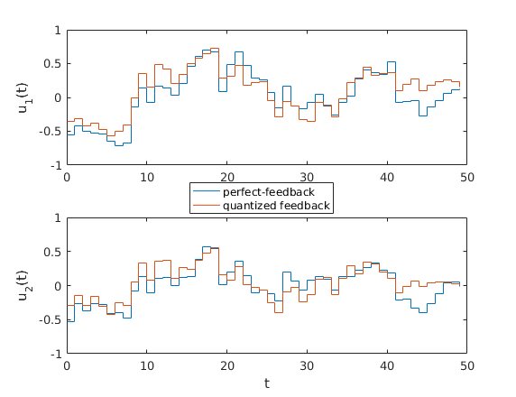
For this example we also implement the perfect state-feedback strategy, i.e., the controllers had a perfect measurement as opposed to quantized measurements. The deviation in the state trajectories and control inputs between the optimal perfect feedback scenario and optimal quantized are shown in Figures 8 and 9. Combining Figures 7, 8 and 9 we notice that by optimally using the quantizers, the control and state trajectories are able to mimic the perfect-feedback trajectory very closely. Since the quantizers considered in this example have 2, 4 and 8 quantization levels, the number of bits required to transmit the measurements will be 1, 2 and 3 bits respectively. For this example, the average bit rate (bits per sample) is (1/T)​∑i=0T−1θti​log2​ℓi=2.22(1/T)\sum_{i=0}^{T-1}\theta^{i}_{t}\log_{2}\ell_{i}=2.22.

Refer to caption
Fig. 8: Top: First component of the state under perfect feedback (blue) and quantized feedback (red). Down: Second component of the state under perfect feedback (blue) and quantized feedback (red).
Refer to caption
Fig. 9: Top: First component of control input under perfect feedback (blue) and quantized feedback (red). Down: Second component of control input under perfect feedback (blue) and quantized feedback (red).

V Discussion and Extensions

V-A Partial Noisy Observations

In this work we have assumed that perfect state measurements are available at the sensor prior to quantization and the communication channel is error-free and not susceptible delay and distortion. The assumption on the availability of perfect state measurement can be dropped and the proposed framework can readily be extended to partially observed noise corrupted sensory measurements. In order to incorporate partial observation where process noise WtW_{t} is not readily computable one needs to construct a different signal from the noisy observations and quantize that specific signal for communication. A detailed study on partially observable systems can be found in our recent work [32].

V-B Delay and Distortion

Two major aspects in considering a digital communication network is delay in the transmission and distortion. In this paper, we have not considered either of these aspects and rather considered an ideal network with zero delay and no distortion in the channel. Although we have not considered the effects of delay explicitly, this framework can easily be extended to the scenario where delay is present. In the presence of network delay, the information available at the controller will be affected since some of the measurements arrival will be delayed and hence the state estimation will be affected. The detailed discussion on the effects of delay is beyond the scope of this work, and the interested readers are directed to our follow-up work in [32].

In order of discuss the effects on channel distortion, let us assume that the channel input alphabet is ℐ=∪i=1M𝒬i\mathcal{I}=\cup_{i=1}^{M}\mathcal{Q}^{i} where channel output alphabet is 𝒪\mathcal{O},66 6 For simplicity, one may assume that 𝒪=ℐ\mathcal{O}=\mathcal{I} i.e., the channel accepts the input qjiq^{i}_{j} from the quantizers and maps it to one of the outputs o∈𝒪o\in\mathcal{O} based on the probability distribution pc​(o|qji)p_{c}(o|q^{i}_{j}). pc(⋅|⋅)p_{c}(\cdot|\cdot) is the channel characteristic which is known and hence, upon receiving an alphabet o∈𝒪o\in\mathcal{O}, we can compute the posterior distribution p⁡(qji|o)p(q^{i}_{j}|o) by Baye’s rule. Thus, if at time tt, the noise Wt−1W_{t-1} is quantized and the controller receives ot∈𝒪o_{t}\in\mathcal{O}, then

𝖤⁡[Wt−1|ot]\displaystyle\mathsf{E}[W_{t-1}~|~o_{t}] =𝖤[𝖤[Wt−1|qji,ot]|ot]\displaystyle=\mathsf{E}\left[\mathsf{E}[W_{t-1}~|~q^{i}_{j},o_{t}]~|o_{t}\right]
=∑i=1M∑j=1ℓi𝖤⁡[Wt−1|qji]​p​(qji|ot).\displaystyle=\sum_{i=1}^{M}\sum_{j=1}^{\ell_{i}}\mathsf{E}[W_{t-1}~|~q_{j}^{i}]p(q^{i}_{j}~|~o_{t}).

In the case of no distortion, we trivially have ot=qkio_{t}=q^{i}_{k} if the input to the channel at time tt was qkiq^{i}_{k}, and hence 𝖤⁡[Wt−1|ot]=𝖤⁡[Wt−1|gi​(Wt−1)]\mathsf{E}[W_{t-1}~|~o_{t}]=\mathsf{E}[W_{t-1}|g_{i}(W_{t-1})] as given in (6).

V-C Choice of Quantizers

The aim of this paper is to select the best quantizer from a given set of quantizers. It is assumed that such a set of quantizers is designed a priori. An interesting research topic is the design of such a set of possible quantizers. From the analysis in this paper, one can immediately see that the cost function is reduced to the form of

J⁡(𝒰∗,Θ∗)=𝖤⁡[X0T​P0​X0]+r0+𝖤⁡[∑t=0T−1Δt∗T​Nt​Δt∗+θt∗T​Λ]\displaystyle J(\mathcal{U}^{*},\Theta^{*})=\mathsf{E}[X_{0}^{\mbox{\tiny\sf T}}P_{0}X_{0}]+r_{0}+\mathsf{E}\left[\sum_{t=0}^{T-1}{\Delta_{t}^{*}}^{\mbox{\tiny\sf T}}N_{t}\Delta_{t}^{*}+{\theta_{t}^{*}}^{\mbox{\tiny\sf T}}\Lambda\right] (33)

where the distribution of Δt∗\Delta^{*}_{t} (and hence 𝖤⁡[Δt∗​Δt∗T]\mathsf{E}[\Delta^{*}_{t}{\Delta^{*}_{t}}^{\mbox{\tiny\sf T}}]) depends on the quantizer parameters. Thus, one can re-write (33) as an explicit function of these parameters, and may further optimize J⁡(𝒰∗,Θ∗)J(\mathcal{U}^{*},\Theta^{*}) with respect to these parameters to find the best set of quantizers. Although, at least in principle, such a method to directly design the quantization set is possible, it can be computationally expensive.

VI CONCLUSIONS

In this work, we have considered a classical quantization-based LQG problem with a positive quantization cost. The problem is to choose an optimal quantizer among a set of available quantizers that minimizes the combined cost of quantization and control performance. We have shown that the optimal controller exhibits a separation principle and it has a linear relationship with the estimate of the state. The optimal gains are found by solving the classical Riccati equation associated with the LQG problem. We have also shown that the optimal selection for the quantizers can be found by solving an auxiliary MDP problem that can be solved independently from the controller synthesis problem. A closed-form solution to the MDP problem is not available at this point. Instead, we provided some structural properties of the value function associated with the MDP. These structural properties can be exploited for the purpose of value function estimation.

We also considered a version of the problem, where the quantization selection is done based on limited information – which we refer to as the quantized measurement information structure. We showed that, under such an information pattern, the controller structure remains unchanged, and the optimal quantization selection can be solved offline.

APPENDIX

Lemma VI.1

Let X:Ω→ℝnxX:\Omega\to\mathbb{R}^{n_{x}} and W:Ω→ℝnwW:\Omega\to\mathbb{R}^{n_{w}} be two independent random variables defined over the probability space (Ω,ℱ,𝖯)(\Omega,\mathcal{F},\mathsf{P}), and let f:ℝnx→ℝnwf:\mathbb{R}^{n_{x}}\to\mathbb{R}^{n_{w}} be a measurable function. Let {ψ1​(⋅),…,ψM​(⋅)}\{\psi^{1}(\cdot),\ldots,\psi^{M}(\cdot)\} be MM measurable functions from ℝnw\mathbb{R}^{n_{w}} to ℝ\mathbb{R}. Then there exists a function ψ~:ℝnw→ℝ∪{−∞,+∞}\tilde{\psi}:\mathbb{R}^{n_{w}}\to\mathbb{R}\cup\{-\infty,+\infty\} such that

𝖤⁡[mini⁡{ψi​(f⁡(X)+W)}|X]=ψ~​(f⁡(X)).\displaystyle\mathsf{E}\left[\min_{i}\{\psi^{i}(f(X)+W)\}~\big|X\right]=\tilde{\psi}(f(X)).
Proof:

Let us denote

RiΨ={w∈ℝnw|ψi(w)≤ψj(w),j=1,2,…,M},\displaystyle R^{\Psi}_{i}=\{w\in\mathbb{R}^{n_{w}}~|~\psi^{i}(w)\leq\psi^{j}(w),j=1,2,\ldots,M\},

so that

∪i=1MRΨi=ℝnw.\displaystyle\cup_{i=1}^{M}R^{\Psi}_{i}=\mathbb{R}^{n_{w}}.

Note that RiΨR^{\Psi}_{i} and RjΨR^{\Psi}_{j} may not necessarily be disjoint for all i,ji,j. For all y∈Rnwy\in R^{n_{w}}, let us define RiΨ(y)={w∈ℝnw|ψi(y+w)≤ψj(y+w),j=1,2,…,M}R^{\Psi}_{i}(y)=\{w\in\mathbb{R}^{n_{w}}~|~\psi^{i}(y+w)\leq\psi^{j}(y+w),j=1,2,\ldots,M\}. One may think of RiΨ​(y)R^{\Psi}_{i}(y) as the translation of the set RiΨR^{\Psi}_{i} by the vector yy. It is also true that ∪i=1MRiΨ(y)=ℝnw\cup_{i=1}^{M}R^{\Psi}_{i}(y)=\mathbb{R}^{n_{w}} for all y∈ℝnwy\in\mathbb{R}^{n_{w}}. If RiΨ​(y)∩RjΨ​(y)≠∅R^{\Psi}_{i}(y)\cap R^{\Psi}_{j}(y)\neq\varnothing for some yy, then we randomly assign the elements of the set RiΨ​(y)∩RjΨ​(y)R^{\Psi}_{i}(y)\cap R^{\Psi}_{j}(y) either to RiΨ​(y)R^{\Psi}_{i}(y) or to RjΨ​(y)R^{\Psi}_{j}(y). Let us denote these sets to be {R~iΨ​(y)}i=1M\{\tilde{R}^{\Psi}_{i}(y)\}_{i=1}^{M} after this random assignment. The random assignment is to ensure R~iΨ​(y)∩R~jΨ​(y)=∅\tilde{R}^{\Psi}_{i}(y)\cap\tilde{R}^{\Psi}_{j}(y)=\varnothing. However, we still have ∪i=1MR~iΨ(y)=ℝnw\cup_{i=1}^{M}\tilde{R}^{\Psi}_{i}(y)=\mathbb{R}^{n_{w}} and

R~iΨ(y)={w∈ℝnw|\displaystyle\tilde{R}^{\Psi}_{i}(y)=\{w\in\mathbb{R}^{n_{w}}~|~ ψi​(y+w)≤ψj​(y+w),\displaystyle\psi^{i}(y+w)\leq\psi^{j}(y+w),
j=1,2,…,M}.\displaystyle j=1,2,\ldots,M\}.

Using {R~iΨ​(y)}i=1M\{\tilde{R}^{\Psi}_{i}(y)\}_{i=1}^{M} as a partition of ℝnw\mathbb{R}^{n_{w}}, we can write

𝖤⁡[mini⁡{ψi​(f⁡(X)+W)}|X]=∫ℝnwmini⁡{ψi​(y+w)}​𝑑𝖯​(w),\displaystyle\mathsf{E}\left[\min_{i}\{\psi^{i}(f(X)+W)\}~\big|X\right]=\int_{\mathbb{R}^{n_{w}}}\min_{i}\{\psi^{i}(y+w)\}d\mathsf{P}(w),

where y=f⁡(X)y=f(X) for notational convenience. Therefore,

𝖤⁡[mini⁡{ψi​(f⁡(X)+W)}|X]=\displaystyle\mathsf{E}\left[\min_{i}\{\psi^{i}(f(X)+W)\}~\big|X\right]= ∑i=1M∫R~iΨ​(y)ψi​(y+w)​𝑑𝖯​(w)\displaystyle\sum_{i=1}^{M}\int_{\tilde{R}^{\Psi}_{i}(y)}\psi^{i}(y+w)d\mathsf{P}(w)
≜\displaystyle\triangleq ∑i=1Mψ~i​(y),\displaystyle\sum_{i=1}^{M}\tilde{\psi}_{i}(y),

where we define ψ~i​(y)=∫R~iΨ​(y)ψi​(y+w)​𝑑𝖯​(w)\tilde{\psi}_{i}(y)=\int_{\tilde{R}^{\Psi}_{i}(y)}\psi^{i}(y+w)d\mathsf{P}(w). If we define ψ~​(y)=∑i=1Mψ~i​(y)\tilde{\psi}(y)=\sum_{i=1}^{M}\tilde{\psi}_{i}(y) for all y∈ℝnwy\in\mathbb{R}^{n_{w}}, then

𝖤⁡[mini⁡{ψi​(f⁡(X)+W)}|X]=ψ~​(y)=ψ~​(f⁡(X)).\displaystyle\mathsf{E}\left[\min_{i}\{\psi^{i}(f(X)+W)\}~\big|X\right]=\tilde{\psi}(y)=\tilde{\psi}(f(X)).

∎Under the hypothesis that XX and WW are independent, and {ψi​(⋅)}\{\psi^{i}(\cdot)\} being a set of measurable functions from ℝnw\mathbb{R}^{n_{w}} to ℝ\mathbb{R}, there always exists a measurable function ψ^:ℝnx→ℝ\hat{\psi}:\mathbb{R}^{n_{x}}\to\mathbb{R} such that

𝖤⁡[mini⁡{ψi​(f⁡(X)+W)}|X]=ψ^​(X).\displaystyle\mathsf{E}\left[\min_{i}\{\psi^{i}(f(X)+W)\}~\big|X\right]=\hat{\psi}(X).

The above lemma shows that ψ^\hat{\psi} can be represented as a composition ψ^​(⋅)=ψ~∘f​(⋅)\hat{\psi}(\cdot)=\tilde{\psi}\circ f(\cdot).

VI-A Proof of Theorem III.3

Proof:

Let us note that at k=T−1k=T-1 we have

CT−1​(s)=\displaystyle C_{T-1}(s)= minγT−1θ⁡𝖤⁡[c~​(ST,θT−1)|ST−1=s]\displaystyle\min_{\gamma^{\theta}_{T-1}}\mathsf{E}\left[\tilde{c}(S_{T},\theta_{T-1})~|~S_{T-1}=s\right]
=\displaystyle= minγT−1θ⁡𝖤⁡[STT​N~T−1​ST+θT−1T​Λ|ST−1=s]\displaystyle\min_{\gamma^{\theta}_{T-1}}\mathsf{E}\left[S_{T}^{\mbox{\tiny\sf T}}\tilde{N}_{T-1}S_{T}+\theta_{T-1}^{\mbox{\tiny\sf T}}\Lambda~|S_{T-1}=s\right]
=\displaystyle= minγT−1θ𝖤[∥HST−1−[GT−1​(ST−1)​θT−10]∥N~T−12\displaystyle\min_{\gamma^{\theta}_{T-1}}\mathsf{E}\Big[\Big\|HS_{T-1}-\begin{bmatrix}G_{T-1}(S_{T-1})\theta_{T-1}\\ 0\end{bmatrix}\Big\|^{2}_{\tilde{N}_{T-1}}
+θT−1TΛ|ST−1=s],\displaystyle~~~~+\theta_{T-1}^{\mbox{\tiny\sf T}}\Lambda~|S_{T-1}=s\Big],

where the last equality follows from N~T−1​[0WT−1]=[00]\tilde{N}_{T-1}\begin{bmatrix}0\\ W_{T-1}\end{bmatrix}=\begin{bmatrix}0\\ 0\end{bmatrix}. Recall that H=[AI00]H=\begin{bmatrix}A~~&{I}\\ {0}~~&{0}\end{bmatrix} and Gt​(St)=[w^t−11​(St),w^t−12​(St),…,w^t−1M​(St)]G_{t}(S_{t})=[\hat{w}_{t-1}^{1}(S_{t}),\hat{w}_{t-1}^{2}(S_{t}),\ldots,\hat{w}_{t-1}^{M}(S_{t})] where w^t−1i​(St)=𝖤⁡[Wt−1|gi​(Wt−1)]\hat{w}_{t-1}^{i}(S_{t})=\mathsf{E}[W_{t-1}~|~g_{i}(W_{t-1})], and St=[Δt−1T,Wt−1T]TS_{t}=[\Delta_{t-1}^{\mbox{\tiny\sf T}},W_{t-1}^{\mbox{\tiny\sf T}}]^{\mbox{\tiny\sf T}}. Here we write the argument in w^t−1i​(⋅)\hat{w}^{i}_{t-1}(\cdot) to emphasize the fact that it depends on StS_{t}.

One can verify that

∥\displaystyle\Big\| [GT−1​(ST−1)​θT−10]∥2N~T−1\displaystyle\begin{bmatrix}G_{T-1}(S_{T-1})\theta_{T-1}\\ 0\end{bmatrix}\Big\|^{2}_{\tilde{N}_{T-1}}
=θT−1T​GT−1​(ST−1)T​NT−1​GT−1​(ST−1)​θT−1\displaystyle=\theta_{T-1}^{\mbox{\tiny\sf T}}G_{T-1}(S_{T-1})^{\mbox{\tiny\sf T}}N_{T-1}G_{T-1}(S_{T-1})\theta_{T-1}
=∑i=1M(w^T−2i​(ST−1))T​NT−1​(w^T−2i​(ST−1))​θT−1i\displaystyle=\sum_{i=1}^{M}\big(\hat{w}^{i}_{T-2}(S_{T-1})\big)^{\mbox{\tiny\sf T}}N_{T-1}\big(\hat{w}^{i}_{T-2}(S_{T-1})\big)\theta_{T-1}^{i}
≜G~T−1​(ST−1)​θT−1,\displaystyle\triangleq\tilde{G}_{T-1}(S_{T-1})\theta_{T-1},

where G~T−1​(ST−1)\tilde{G}_{T-1}(S_{T-1}) is the vector [‖w^T−21​(ST−1)‖NT−12,…,‖w^T−2M​(ST−1)‖NT−12][\|\hat{w}^{1}_{T-2}(S_{T-1})\|_{N_{T-1}}^{2},\ldots,\|\hat{w}^{M}_{T-2}(S_{T-1})\|_{N_{T-1}}^{2}].

Thus, after some simplifications,

CT−1​(s)=\displaystyle C_{T-1}(s)= minγT−1θ{ST−1THTN~T−1HST−1\displaystyle\min_{\gamma^{\theta}_{T-1}}\Big\{S_{T-1}^{\mbox{\tiny\sf T}}H^{\mbox{\tiny\sf T}}\tilde{N}_{T-1}HS_{T-1}
−2​ST−1T​[AT​NT−1​GT−1​(ST−1)0]​θT−1\displaystyle-2S_{T-1}^{\mbox{\tiny\sf T}}\begin{bmatrix}A^{\mbox{\tiny\sf T}}{N}_{T-1}G_{T-1}(S_{T-1})\\ {0}\end{bmatrix}\theta_{T-1}
+G~T−1(ST−1)θT−1+θT−1TΛ}\displaystyle+\tilde{G}_{T-1}(S_{T-1})\theta_{T-1}+\theta_{T-1}^{\mbox{\tiny\sf T}}\Lambda\Big\}
=\displaystyle= minγT−1θ⁡{ΨT−1​(ST−1)​θT−1}\displaystyle\min_{\gamma^{\theta}_{T-1}}\Big\{\Psi_{T-1}(S_{T-1})\theta_{T-1}\Big\}
+ST−1T​HT​N~T−1​H​ST−1\displaystyle+S_{T-1}^{\mbox{\tiny\sf T}}H^{\mbox{\tiny\sf T}}\tilde{N}_{T-1}HS_{T-1}

where ΨT−1​(ST−1)=−2​ST−1T​[AT​NT−1​GT−1​(ST−1)0]+G~T−1​(ST−1)+ΛT\Psi_{T-1}(S_{T-1})=-2S_{T-1}^{\mbox{\tiny\sf T}}\begin{bmatrix}A^{\mbox{\tiny\sf T}}{N}_{T-1}G_{T-1}(S_{T-1})\\ {0}\end{bmatrix}+\tilde{G}_{T-1}(S_{T-1})+\Lambda^{\mbox{\tiny\sf T}} is an MM dimensional row vector. Let us denote by ΨT−1​(⋅)=[ψT−1i​(⋅),ψT−12​(⋅),…,ψT−1M​(⋅)]\Psi_{T-1}(\cdot)=[\psi^{i}_{T-1}(\cdot),\psi^{2}_{T-1}(\cdot),\ldots,\psi^{M}_{T-1}(\cdot)], where ψT−1i:ℝ2​n→ℝ\psi^{i}_{T-1}:\mathbb{R}^{2n}\to\mathbb{R} is the ii-th component of ΨT−1\Psi_{T-1}. Thus, minγT−1θ⁡{ΨT−1​(ST−1)​θT−1}=mini⁡{ψT−1i​(ST−1)}\min_{\gamma^{\theta}_{T-1}}\Big\{\Psi_{T-1}(S_{T-1})\theta_{T-1}\Big\}=\min_{i}\{\psi^{i}_{T-1}(S_{T-1})\}. Let

i∗​(ST−1)=arg⁡mini​{ψT−1i​(ST−1)}.\displaystyle i^{*}(S_{T-1})=\arg\min_{i}\{\psi^{i}_{T-1}(S_{T-1})\}.

If i∗​(ST−1)i^{*}(S_{T-1}) is not unique, then without loss of generality, one of the minimizers is randomly selected.77 7 In case there are multiple i∈{0,1,…,M}i\in\{0,1,\ldots,M\} that minimizes mini⁡{ψT−1i​(ST−1)}\min_{i}\{\psi^{i}_{T-1}(S_{T-1})\}, let us introduce the set I∗={i1∗,i2∗,…,il∗}I^{*}=\{i^{*}_{1},i^{*}_{2},\ldots,i^{*}_{l}\} where l≤Ml\leq M, ij∗∈{1,2,…,M}i^{*}_{j}\in\{1,2,\ldots,M\} and each ij∗i^{*}_{j} is a minimizer. In such a case, one can use a randomized policy over this set of minimizers to select the quantizers, i.e., γT−1θ​(ST−1)=bj\gamma^{\theta}_{T-1}(S_{T-1})=b_{j} with probability pj∈[0,1]p_{j}\in[0,1] where j∈I∗j\in I^{*} and ∑j∈I∗pj=1\sum_{j\in I^{*}}p_{j}=1. Nonetheless, the value CT−1​(ST−1)C_{T-1}(S_{T-1}) remains unaffected by the choice of pjp_{j}. It follows

θT−1∗=γT−1θ∗(ST−1)=bi∗​(ST−1),\displaystyle\theta^{*}_{T-1}=\gamma^{\theta*}_{T-1}(S_{T-1})=b_{i^{*}(S_{T-1})},

where bi∈𝒜b_{i}\in\mathcal{A} is the ii-th basis vector in ℝM\mathbb{R}^{M}. Thus,

CT−1​(ST−1)=ST−1T​ΦT−1​ST−1+mini⁡{ψT−1i​(ST−1)},\displaystyle C_{T-1}(S_{T-1})=S_{T-1}^{\mbox{\tiny\sf T}}\Phi_{T-1}S_{T-1}+\min_{i}\{\psi^{i}_{T-1}(S_{T-1})\},

where ΦT−1=HT​N~T−1​H\Phi_{T-1}=H^{\mbox{\tiny\sf T}}\tilde{N}_{T-1}H.

Let us now assume that for some kk it is true that

Ck​(Sk)=SkT​Φk​Sk+mini=1,…,M⁡{ψki​(Sk)}.\displaystyle C_{k}(S_{k})=S_{k}^{\mbox{\tiny\sf T}}\Phi_{k}S_{k}+\min_{i=1,\ldots,M}\{\psi^{i}_{k}(S_{k})\}. (34)

Recall that,

Ck−1​(Sk−1)=minγk−1θ⁡𝖤⁡[SkT​N~k​Sk+θk−1T​Λ+Ck​(Sk)|Sk−1].\displaystyle C_{k-1}(S_{k-1})=\min_{\gamma^{\theta}_{k-1}}\mathsf{E}\Big[S_{k}^{\mbox{\tiny\sf T}}\tilde{N}_{k}S_{k}+\theta_{k-1}^{\mbox{\tiny\sf T}}\Lambda+C_{k}(S_{k})~|S_{k-1}\Big].

Using the hypothesis, let us replace Ck​(Sk)C_{k}(S_{k}) in the above equation, and consequently

Ck−1​(Sk−1)=\displaystyle C_{k-1}(S_{k-1})= minγk−1θ𝖤[SkT(N~k+Φk)Sk+θk−1TΛ\displaystyle\min_{\gamma^{\theta}_{k-1}}\mathsf{E}\Big[S_{k}^{\mbox{\tiny\sf T}}(\tilde{N}_{k}+\Phi_{k})S_{k}+\theta_{k-1}^{\mbox{\tiny\sf T}}\Lambda
+mini=1,…,M{ψki(Sk)}|Sk−1].\displaystyle+\min_{i=1,\ldots,M}\{\psi^{i}_{k}(S_{k})\}~|~S_{k-1}\Big]. (35)

Using the dynamics of StS_{t} in (III-A) one can write Sk=f0​(k−1,Sk−1,θk−1)+[0Wk−1]S_{k}=f_{0}(k-1,S_{k-1},\theta_{k-1})+\begin{bmatrix}0\\ W_{k-1}\end{bmatrix}. The expression for f0​(⋅,⋅,⋅)f_{0}(\cdot,\cdot,\cdot) can be obtained from (III-A)

f0​(t,S,θ)=H​S−[Gt​(S)​θ0].\displaystyle f_{0}(t,S,\theta)=HS-\begin{bmatrix}G_{t}(S)\theta\\ 0\end{bmatrix}.

Since Sk−1S_{k-1} and Wk−1W_{k-1} are independent random variables and θk−1=γk−1θ​(Sk−1)\theta_{k-1}=\gamma^{\theta}_{k-1}(S_{k-1}), we can use Lemma VI.188 8 Use Sk−1S_{k-1} as XX and f0​(K−1,Sk−1,γk−1θ​(Sk−1))f_{0}(K-1,S_{k-1},\gamma^{\theta}_{k-1}(S_{k-1})) as the f⁡(X)f(X) in Lemma VI.1. to conclude that there exists a function ψ~k:ℝ2​n→ℝ\tilde{\psi}_{k}:\mathbb{R}^{2n}\to\mathbb{R} such that

ψ~k​(f0​(k−1,Sk−1,θk−1))=𝖤⁡[mini=1,…,M⁡{ψki​(Sk)}|Sk−1].\displaystyle\tilde{\psi}_{k}(f_{0}(k-1,S_{k-1},\theta_{k-1}))=\mathsf{E}\left[\min_{i=1,\ldots,M}\{\psi^{i}_{k}(S_{k})\}~|~S_{k-1}\right]. (36)

Since θk−1∈𝒜={b1,b2,…,bM}\theta_{k-1}\in\mathcal{A}=\{b_{1},b_{2},\ldots,b_{M}\}, we define

ψ~ki​(Sk−1)≜ψ~k​(f0​(k−1,Sk−1,bi)).\displaystyle\tilde{\psi}^{i}_{k}(S_{k-1})\triangleq\tilde{\psi}_{k}(f_{0}(k-1,S_{k-1},b_{i})).

Therefore,

ψ~k​(f0​(k−1,Sk−1,θk−1))=∑i=1Mψ~ki​(Sk−1)​θk−1i.\displaystyle\tilde{\psi}_{k}(f_{0}(k-1,S_{k-1},\theta_{k-1}))=\sum_{i=1}^{M}\tilde{\psi}^{i}_{k}(S_{k-1})\theta^{i}_{k-1}. (37)

Following similar steps as before, it can be shown that

𝖤\displaystyle\mathsf{E} [SkT​(N~k+Φk)​Sk|Sk−1]=Sk−1T​HT​(N~k+Φk)​H​Sk−1\displaystyle\left[S_{k}^{\mbox{\tiny\sf T}}(\tilde{N}_{k}+\Phi_{k})S_{k}~|S_{k-1}\right]=S_{k-1}^{\mbox{\tiny\sf T}}H^{\mbox{\tiny\sf T}}(\tilde{N}_{k}+\Phi_{k})HS_{k-1}
+𝖤⁡[[0Wk−1]T​(N~k+Φk)​[0Wk−1]]\displaystyle+\mathsf{E}\left[\begin{bmatrix}0\\ W_{k-1}\end{bmatrix}^{\mbox{\tiny\sf T}}(\tilde{N}_{k}+\Phi_{k})\begin{bmatrix}0\\ W_{k-1}\end{bmatrix}\right]
−2∑i=1MSk−1THT(N~k+Φk)[w^k−2i​(Sk−1)0]θk−1i\displaystyle-2\sum_{i=1}^{M}S_{k-1}^{\mbox{\tiny\sf T}}H^{\mbox{\tiny\sf T}}(\tilde{N}_{k}+\Phi_{k})\begin{bmatrix}\hat{w}^{i}_{k-2}(S_{k-1})\\ 0\end{bmatrix}\theta^{i}_{k-1}
+∑i=1M[w^k−2i​(Sk−1)0]T(N~k+Φk)[w^k−2i​(Sk−1)0]θk−1i.\displaystyle+\sum_{i=1}^{M}\begin{bmatrix}\hat{w}^{i}_{k-2}(S_{k-1})\\ 0\end{bmatrix}^{\mbox{\tiny\sf T}}(\tilde{N}_{k}+\Phi_{k})\begin{bmatrix}\hat{w}^{i}_{k-2}(S_{k-1})\\ 0\end{bmatrix}\theta^{i}_{k-1}.

Using the fact 𝖤⁡[Wk−1​Wk−1T]=𝒲\mathsf{E}[W_{k-1}W_{k-1}^{\mbox{\tiny\sf T}}]=\mathcal{W}, we obtain

𝖤\displaystyle\mathsf{E} [SkT​(N~k+Φk)​Sk|Sk−1]=Sk−1T​HT​(N~k+Φk)​H​Sk−1\displaystyle\left[S_{k}^{\mbox{\tiny\sf T}}(\tilde{N}_{k}+\Phi_{k})S_{k}~|S_{k-1}\right]=S_{k-1}^{\mbox{\tiny\sf T}}H^{\mbox{\tiny\sf T}}(\tilde{N}_{k}+\Phi_{k})HS_{k-1}
+tr⁡((N~k+Φk)​[000𝒲])\displaystyle+{\rm{tr}}\Big((\tilde{N}_{k}+\Phi_{k})\begin{bmatrix}{0}&{0}\\ {0}&\mathcal{W}\end{bmatrix}\Big)
−2∑i=1MSk−1THT(N~k+Φk)[w^k−2i​(Sk−1)0]θk−1i\displaystyle-2\sum_{i=1}^{M}S_{k-1}^{\mbox{\tiny\sf T}}H^{\mbox{\tiny\sf T}}(\tilde{N}_{k}+\Phi_{k})\begin{bmatrix}\hat{w}^{i}_{k-2}(S_{k-1})\\ 0\end{bmatrix}\theta^{i}_{k-1}
+∑i=1M[w^k−2i​(Sk−1)0]T(N~k+Φk)[w^k−2i​(Sk−1)0]θk−1i.\displaystyle+\sum_{i=1}^{M}\begin{bmatrix}\hat{w}^{i}_{k-2}(S_{k-1})\\ 0\end{bmatrix}^{\mbox{\tiny\sf T}}(\tilde{N}_{k}+\Phi_{k})\begin{bmatrix}\hat{w}^{i}_{k-2}(S_{k-1})\\ 0\end{bmatrix}\theta^{i}_{k-1}. (38)

Let us now define ψk−1i​(Sk−1)\psi^{i}_{k-1}(S_{k-1}) as follows

ψk−1i​(Sk−1)\displaystyle\psi^{i}_{k-1}(S_{k-1}) =ψ~ki​(Sk−1)+λi+tr⁡((N~k+Φk)​[000𝒲])\displaystyle=\tilde{\psi}^{i}_{k}(S_{k-1})+\lambda_{i}+{\rm{tr}}\Big((\tilde{N}_{k}+\Phi_{k})\begin{bmatrix}{0}&{0}\\ {0}&\mathcal{W}\end{bmatrix}\Big)
+[w^k−2i​(Sk−1)0]T​(N~k+Φk)​[w^k−2i​(Sk−1)0]\displaystyle+\begin{bmatrix}\hat{w}^{i}_{k-2}(S_{k-1})\\ 0\end{bmatrix}^{\mbox{\tiny\sf T}}(\tilde{N}_{k}+\Phi_{k})\begin{bmatrix}\hat{w}^{i}_{k-2}(S_{k-1})\\ 0\end{bmatrix}
−2​Sk−1T​HT​(N~k+Φk)​[w^k−2i​(Sk−1)0].\displaystyle-2S_{k-1}^{\mbox{\tiny\sf T}}H^{\mbox{\tiny\sf T}}(\tilde{N}_{k}+\Phi_{k})\begin{bmatrix}\hat{w}^{i}_{k-2}(S_{k-1})\\ 0\end{bmatrix}. (39)

Using (36), (37), (VI-A) and (VI-A) we can rewrite (VI-A) as

Ck−1​(Sk−1)=Sk−1T​Φk−1​Sk−1+minγk−1θ⁡{∑i=1Mψk−1i​(Sk−1)​θk−1i},\displaystyle C_{k-1}(S_{k-1})=S_{k-1}^{\mbox{\tiny\sf T}}\Phi_{k-1}S_{k-1}+\min_{\gamma^{\theta}_{k-1}}\{\sum_{i=1}^{M}\psi^{i}_{k-1}(S_{k-1})\theta^{i}_{k-1}\},

where Φk−1=HT​(N~k+Φk)​H\Phi_{k-1}=H^{\mbox{\tiny\sf T}}(\tilde{N}_{k}+\Phi_{k})H.

Let us denote

ik−1∗​(Sk−1)=arg⁡mini​{ψk−1i​(Sk−1)}.\displaystyle i^{*}_{k-1}(S_{k-1})=\arg\min_{i}\{\psi^{i}_{k-1}(S_{k-1})\}.

If ik−1∗​(Sk−1)i^{*}_{k-1}(S_{k-1}) is not unique, then without loss of generality one of the minimizers is randomly selected. Therefore,

θk−1∗=γk−1θ∗(Sk−1)=bik−1∗​(Sk−1),\displaystyle\theta^{*}_{k-1}=\gamma^{\theta*}_{k-1}(S_{k-1})=b_{i^{*}_{k-1}(S_{k-1})},

where bi∈𝒜b_{i}\in\mathcal{A} is the ii-th basis vector in ℝM\mathbb{R}^{M}. Thus,

Ck−1​(Sk−1)=Sk−1T​Φk−1​Sk−1+mini⁡{ψk−1i​(Sk−1)},\displaystyle C_{k-1}(S_{k-1})=S_{k-1}^{\mbox{\tiny\sf T}}\Phi_{k-1}S_{k-1}+\min_{i}\{\psi^{i}_{k-1}(S_{k-1})\},

and Ck​(Sk)C_{k}(S_{k}) is indeed of the form of (34).

Let us now define the region

ℛ~k−1i={s∈ℝ2​n|ψk−1i​(s)≤ψk−1j​(s)​∀j}⊆ℝ2​n,\displaystyle\tilde{\mathcal{R}}^{i}_{k-1}=\{s\in\mathbb{R}^{2n}~|~\psi^{i}_{k-1}(s)\leq\psi^{j}_{k-1}(s)~~\forall j\}\subseteq\mathbb{R}^{2n},

and let us also define

ℛk−11\displaystyle\mathcal{R}^{1}_{k-1} =ℛ~k−11,\displaystyle=\tilde{\mathcal{R}}^{1}_{k-1},
ℛk−1i\displaystyle\mathcal{R}^{i}_{k-1} =ℛ~k−1i∖∪j=1i−1(ℛ~k−1i∩ℛ~k−1j).\displaystyle=\tilde{\mathcal{R}}^{i}_{k-1}\setminus\cup_{j=1}^{i-1}(\tilde{\mathcal{R}}^{i}_{k-1}\cap\tilde{\mathcal{R}}^{j}_{k-1}).

It can be verified that ∪i=1Mℛ~ik−1=∪i=1Mℛik−1=ℝ2​n\cup_{i=1}^{M}\tilde{\mathcal{R}}^{i}_{k-1}=\cup_{i=1}^{M}{\mathcal{R}}^{i}_{k-1}=\mathbb{R}^{2n}. Moreover, ℛk−1i∩ℛk−1j=∅\mathcal{R}^{i}_{k-1}\cap\mathcal{R}^{j}_{k-1}=\varnothing for all i,j∈{1,2,…,M}i,j\in\{1,2,\ldots,M\}. By construction, if Sk∈ℛk−1jS_{k}\in\mathcal{R}^{j}_{k-1} for some jj, then ψk−1j​(Sk)=mini⁡{ψk−1i​(Sk)}\psi^{j}_{k-1}(S_{k})=\min_{i}\{\psi^{i}_{k-1}(S_{k})\}. Thus, γk−1θ∗(Sk)=bj\gamma^{\theta*}_{k-1}(S_{k})=b_{j} is an optimal strategy. In other words, θk−1i∗=1ℛk−1i(Sk)\theta^{i*}_{k-1}=1_{\mathcal{R}^{i}_{k-1}}(S_{k}) is optimal. ∎

References

  • [1] V. S. Borkar and S. K. Mitter, “LQG control with communication constraints,” in Communications, Computation, Control, and Signal Processing. Springer, 1997, pp. 365–373.
  • [2] S. Tatikonda, “Control under communication constraints,” Ph.D. dissertation, Massachusetts Institute of Technology, 2000.
  • [3] S. Tatikonda, A. Sahai, and S. Mitter, “Control of LQG systems under communication constraints,” in Proceedings of the 37th IEEE Conference on Decision and Control, 1998, pp. 1165–1170, Tampa, USA.
  • [4] G. N. Nair and R. J. Evans, “Stabilizability of stochastic linear systems with finite feedback data rates,” SIAM Journal on Control and Optimization, vol. 43, no. 2, pp. 413–436, 2004.
  • [5] S. Tatikonda, A. Sahai, and S. Mitter, “Stochastic linear control over a communication channel,” IEEE Transactions on Automatic Control, vol. 49, no. 9, pp. 1549–1561, 2004.
  • [6] V. Kostina and B. Hassibi, “Rate-cost tradeoffs in control,” IEEE Transactions on Automatic Control, 2019.
  • [7] E. I. Silva, M. S. Derpich, and J. Ostergaard, “A framework for control system design subject to average data-rate constraints,” IEEE Transactions on Automatic Control, vol. 56, no. 8, pp. 1886–1899, 2010.
  • [8] E. I. Silva, M. S. Derpich, J. Østergaard, and M. A. Encina, “A characterization of the minimal average data rate that guarantees a given closed-loop performance level,” IEEE Transactions on Automatic Control, vol. 61, no. 8, pp. 2171–2186, 2015.
  • [9] R. E. Curry, Estimation and Control with Quantized Measurements. MIT press Cambridge, MA, 1970.
  • [10] F. Schweppe, “Recursive state estimation: Unknown but bounded errors and system inputs,” IEEE Transactions on Automatic Control, vol. 13, no. 1, pp. 22–28, 1968.
  • [11] P. Moroney, Issues in the Implementation of Digital Compensators. MIT Press, 1983.
  • [12] D. F. Delchamps, “Extracting state information from a quantized output record,” Systems & Control Letters, vol. 13, no. 5, pp. 365–372, 1989.
  • [13] D. Williamson and K. Kadiman, “Optimal finite wordlength linear quadratic regulation,” IEEE Transactions on Automatic Control, vol. 34, no. 12, pp. 1218–1228, 1989.
  • [14] K. Liu, R. E. Skelton, and K. Grigoriadis, “Optimal controllers for finite wordlength implementation,” IEEE Transactions on Automatic Control, vol. 37, no. 9, pp. 1294–1304, 1992.
  • [15] T. Tanaka, K. H. Johansson, and M. Skoglund, “Optimal block length for data-rate minimization in networked lqg control,” IFAC-PapersOnLine, vol. 49, no. 22, pp. 133–138, 2016.
  • [16] D. F. Delchamps, “Stabilizing a linear system with quantized state feedback,” IEEE Transactions on Automatic Control, vol. 35, no. 8, pp. 916–924, 1990.
  • [17] W. S. Wong and R. W. Brockett, “Systems with finite communication bandwidth constraints. I. State estimation problems,” IEEE Transactions on Automatic Control, vol. 42, no. 9, pp. 1294–1299, 1997.
  • [18] ——, “Systems with finite communication bandwidth constraints. II. Stabilization with limited information feedback,” IEEE Transactions on Automatic Control, vol. 44, no. 5, pp. 1049–1053, 1999.
  • [19] H. Ishii and B. A. Francis, “Quadratic stabilization of sampled-data systems with quantization,” Automatica, vol. 39, no. 10, pp. 1793–1800, 2003.
  • [20] K. Li and J. Baillieul, “Robust quantization for digital finite communication bandwidth (DFCB) control,” IEEE Transactions on Automatic Control, vol. 49, no. 9, pp. 1573–1584, 2004.
  • [21] F. Fagnani and S. Zampieri, “Stabilizing quantized feedback with minimal information flow: the scalar case,” in Proc. of MTNS Conference, 2002.
  • [22] N. Elia and S. K. Mitter, “Stabilization of linear systems with limited information,” IEEE Transactions on Automatic Control, vol. 46, no. 9, pp. 1384–1400, 2001.
  • [23] R. W. Brockett and D. Liberzon, “Quantized feedback stabilization of linear systems,” IEEE Transactions on Automatic Control, vol. 45, no. 7, pp. 1279–1289, 2000.
  • [24] D. Liberzon, “On stabilization of linear systems with limited information,” IEEE Transactions on Automatic Control, vol. 48, no. 2, pp. 304–307, 2003.
  • [25] G. N. Nair and R. J. Evans, “Exponential stabilisability of finite-dimensional linear systems with limited data rates,” Automatica, vol. 39, no. 4, pp. 585–593, 2003.
  • [26] J. Pearson, J. P. Hespanha, and D. Liberzon, “Control with minimal cost-per-symbol encoding and quasi-optimality of event-based encoders,” IEEE Transactions on Automatic Control, vol. 62, no. 5, pp. 2286–2301, 2017.
  • [27] M. Aoki and M. T. Li, “Optimal discrete-time control system with cost for observation,” IEEE Transactions on Automatic Control, vol. 14, no. 2, pp. 165–175, 1969.
  • [28] R. Bansal and T. Başar, “Simultaneous design of measurement and control strategies for stochastic systems with feedback,” Automatica, vol. 25, no. 5, pp. 679–694, 1989.
  • [29] T. Fischer, “Optimal quantized control,” IEEE Transactions on Automatic Control, vol. 27, no. 4, pp. 996–998, 1982.
  • [30] A. Gersho and R. M. Gray, Vector Quantization and Signal Compression. Springer Science & Business Media, 2012, vol. 159.
  • [31] Y. Linde, A. Buzo, and R. Gray, “An algorithm for vector quantizer design,” IEEE Transactions on Communications, vol. 28, no. 1, pp. 84–95, 1980.
  • [32] D. Maity and P. Tsiotras, “Optimal controller and quantizer selection for partially observable linear-quadratic-gaussian systems,” arXiv preprint arXiv:1909.13609, 2019.
[Uncaptioned image] Dipankar Maity received the B.E. degree in Electronics and Telecommunication Engineering from Jadavpur University, India in 2013, and the Ph.D degree in Electrical and Computer Engineering from University of Maryland College Park, USA in 2018. During his Ph.D, he was a visiting scholar at the Technische Universität München (TUM) and at the Royal Institute of Technology (KTH) Sweden. Currently, he is a Postdoctoral Fellow at Georgia Institute of Technology. His research interests include temporal logic based controller synthesis, Control with logical constraints, control with communication constraints, intermittent-feedback control, event-triggered control, stochastic games, and integration of these ideas in the context of cyber-physical-systems.
[Uncaptioned image] Panagiotis Tsiotras is the David and Andrew Lewis Chair Professor in the D. Guggenheim School of Aerospace Engineering at the Georgia Institute of Technology (Georgia Tech), and the Director of the Dynamics and Controls Systems Laboratory (DCSL) in the same school, as well as Associate Director of the Institute for Robotics and Intelligent Machines at Georgia Tech. He holds degrees in Aerospace Engineering, Mechanical Engineering, and Mathematics. He has held visiting research appointments at MIT, JPL, INRIA Rocquencourt, and Mines ParisTech. His research interests include optimal control of nonlinear systems and ground, aerial and space vehicle autonomy. He has served in the Editorial Boards of the Transactions on Automatic Control, the IEEE Control Systems Magazine, the AIAA Journal of Guidance, Control and Dynamics, the Dynamic Games and Applications, and Dynamics and Control. He is the recipient of the NSF CAREER award, the Outstanding Aerospace Engineer award from Purdue, and the Technical Excellence Award in Aerospace Control from IEEE. He is a Fellow of AIAA, IEEE, and AAS, and a member of the Phi Kappa Phi, Tau Beta Pi, and Sigma Gamma Tau Honor Societies.