Rapid Detection of Hot-spot by Tensor Decomposition on Space and Circular Time with Application to Weekly Gonorrhea data

In this section, we introduce basic notations, definitions, and operators in tensor (multi-linear) algebra that are useful in this paper. Throughout the paper, scalars are denoted by lowercase letters (e.g., $\theta$), vectors are denoted by lowercase boldface letters ($\boldsymbol{\theta}$), matrices are denoted by uppercase boldface letter ($\boldsymbol{\Theta}$), and tensors by curlicue letter ($\vartheta$). For example, an order-$N$ tensor is represented by $\vartheta\in\mathbb{R}^{I_{1}\times\cdots\times I_{N}}$, where $I_{k}$ represent the mode-$n$ dimension of $\vartheta$ for $k=1,\ldots,N$.

The mode-$n$ product of a tensor $\vartheta\in\mathbb{R}^{I_{1}\times\ldots\times I_{N}}$ by a matrix $\mathbf{B}\in\mathbb{R}^{J_{n}\times I_{n}}$ is a tensor $\mathcal{A}\in\mathbb{R}^{I_{1}\times\ldots I_{n-1}\times J_{n}\times I_{n+1}\times\ldots I_{N}}$, denoted as $\mathcal{A}=\vartheta\times_{n}\mathbf{B},$ where each entry of $\mathcal{A}$ is defined as the sum of products of corresponding entries in $\mathcal{A}$ and $\mathbf{B}$: $\mathcal{A}_{i_{1},\ldots,i_{n-1},j_{n},i_{n+1},\ldots,i_{N}}=\sum_{i_{n}}\vartheta_{i_{1},\ldots,i_{N}}\mathbf{B}_{j_{n},i_{n}}$. Here we use the notation $\mathbf{B}_{j_{n},i_{n}}$ to refer the $(j_{n},i_{n})$-th entry in matrix $\mathbf{B}$. The notation $\vartheta_{i_{1},\ldots,i_{N}}$ is used to refer to the entry in tensor $\vartheta$ with index $(i_{1},\ldots,i_{N})$. The notation $\mathcal{A}_{i_{1},\ldots,i_{n-1},j_{n},i_{n+1},\ldots,i_{N}}$ is used to refer the entry in tensor $\mathcal{A}$ with index $(i_{1},\ldots,i_{n-1},j_{n},i_{n+1},\ldots,i_{N})$.

The mode-n unfold of the tensor $\vartheta\in\mathbb{R}^{I_{1}\times\ldots\times I_{N}}$ is denoted by $\vartheta_{(n)}\in\mathbb{R}^{I_{n}\times(I_{1}\times\ldots I_{n-1}\times I_{n+1}\times I_{N})},$ where the column vector of $\vartheta_{(n)}$ are the mode-n vector of $\vartheta$. The mode-n vector of $\vartheta$ are defined as the $I_{n}$ dimensional vector obtained from $\vartheta$ by varying the index $i_{n}$ while keeping all the other indices fixed. For example, $\vartheta_{:,2,3}$ is a model-1 vector.

A very useful technique in the tensor algebra is the Tucker decomposition, which decomposes a tensor into a core tensor multiplied by matrices along each mode: $\mathcal{Y}=\vartheta\times_{1}\mathbf{B}^{(1)}\times_{2}\mathbf{B}^{(2)}\cdots\times_{N}\mathbf{B}^{(N)}$, where $\mathbf{B}^{(n)}$ is an orthogonal $I_{n}\times I_{n}$ matrix and is a principal component mode-$n$ for $n=1,\ldots,N$. Tensor product can be represented equivalently by a Kronecker product, i.e., $\mathrm{vec}(\mathcal{Y})=(\mathbf{B}^{(N)}\otimes\cdots\otimes\mathbf{B}^{(1)})\mathrm{vec}(\vartheta)$, where $\mathrm{vec}(\cdot)$ is the vectorized operator. Finally, the definition of Kronecker product is as follow: Suppose $\mathbf{B}_{1}\in\mathbb{R}^{m\times n}$ and $\mathbf{B}_{2}\in\mathbb{R}^{p\times q}$ are matrices, the Kronecker product of these matrices, denoted by $\mathbf{B}_{1}\otimes\mathbf{B}_{2}$, is an $mq\times nq$ block matrix defined by

Our proposed SSR-Tensor model is built on tensors of order three, as it is inspired by the gonorrhea data, which can be represented as a three-dimension tensor $\mathcal{Y}_{n_{1}\times n_{2}\times T}$ with $n_{1}=50$ states, $n_{2}=51$ weeks, and $T=13$ years. Note that the $i$-th,j$-th$, and $k$-th slice of the 3-D tensor along the dimension of state, week, and year can be achieved as $\mathcal{Y}_{i::},\mathcal{Y}_{:j:},\mathcal{Y}_{::k}$ correspondingly, where $i=1\cdots n_{1}$, $j=1\cdots n_{2}$ and $k=1\cdots T$. For simplicity, we denote $\mathbf{Y}_{k}=\mathcal{Y}_{::k}$. We further denote $\mathbf{y}_{k}$ as the vectorized form of $\mathbf{Y}_{k}$, and $\mathbf{y}$ as the vectorized form of $\mathcal{Y}$.

The key idea of our proposed model is to separate the global trend from the local pattern by decomposing the tensor $\mathbf{y}$ into three parts, namely the smooth global trend $\boldsymbol{\mu}$, local hot-spot $\mathbf{h}$, and residual $\mathbf{e}$, i.e. $\mathbf{y}=\boldsymbol{\mu}+\mathbf{h}+\mathbf{e}$. For the first two of the components (e.g. the global trend mean and local hot-spots), we introduce basis decomposition framework to represent the structure of the within correlation in the global background and local hot-spot, also see Yan et al., 2018.

To be more concrete, we assume that global trend mean and local hot-spot can be represented as $\boldsymbol{\mu}=\mathbf{B}_{m}\boldsymbol{\theta}_{m}$ and $\boldsymbol{h}=\mathbf{B}_{h}\boldsymbol{\theta}_{h}$, where $\mathbf{B}_{m}$ and $\mathbf{B}_{h}$ are two bases that will discussed below, and $\boldsymbol{\theta}_{m}$ and $\boldsymbol{\theta}_{h}$ are the model coefficients vector of length $n_{1}n_{2}T$ and needed to be estimated (see Section 5). Here the subscript of m and h are abbreviations for mean and hot-spot. Next, it is useful to discuss how to choose the bases $\mathbf{B}_{m}$ and $\mathbf{B}_{h},$ so as to characterize the complex “within” and “between” correlation or interaction structures. For the “within” correlation structures, we propose to use pre-specified bases, $\mathbf{B}_{m,s}$ and $\mathbf{B}_{h,s}$, for within-state correlation in global trend and hot-spot, where the subscript of s is an abbreviation for states. Similarly, $\mathbf{B}_{m,w}$ and $\mathbf{B}_{h,w}$ are the pre-specified bases for within-correlation of the same week, whereas $\mathbf{B}_{m,y}$ and $\mathbf{B}_{h,y}$ are the bases for within-time correlation over time. As for the “between” interaction, we use tensor product to describe it, i.e, $\mathbf{B}_{m}=\mathbf{B}_{m,s}\otimes\mathbf{B}_{m,w}\otimes\mathbf{B}_{m,y}$ and $\mathbf{B}_{h}=\mathbf{B}_{h,s}\otimes\mathbf{B}_{h,w}\otimes\mathbf{B}_{h,y}$. This Kronecker product has been proved to have better computational efficiency in the tensor response data Kolda and Bader, 2009. Mathematically speaking, all these bases are matrices, which is pre-assigned in our paper. And the choice of bases in shown in Section 6.2. With the well-structured “within” and “between” interaction, our proposed model can be written as:

where $\mathbf{e}{\sim}N(0,\sigma^{2}\mathbf{I})$ is the random noise. Mathematically speaking, both $\mathbf{B}_{m,s}$ and $\mathbf{B}_{h,s}$ are $n_{1}\times n_{1}$ matrix, $\mathbf{B}_{m,w}$ and $\mathbf{B}_{h,w}$ are $n_{2}\times n_{2}$ matrix and $\mathbf{B}_{m,y}$ and $\mathbf{B}_{h,y}$ are $T\times T$ matrix, respectively.

Mathematically, our proposed model in (1) can be rewritten into a tensor format:

where $\vartheta_{m}$ and $\vartheta_{h}$ is the tensor format of $\boldsymbol{\theta}_{m}$ and $\boldsymbol{\theta}_{h}$ with dimensional $n_{1}\times n_{2}\times T$. Accordingly, the $((k-1)n_{1}n_{2}+(i-1)n_{1}+j)$-th entry of $\boldsymbol{\theta}_{h}$, $\boldsymbol{\theta}_{m}$ can estimate the global mean and hot-spot in $i$-th state and $j$-th week in $k$-th year respectively. The tensor representation in equation (2) allows us to develop computationally efficient methods for estimation and prediction.

With the proposed SSR-Tensor model above, we can now discuss the estimation of hot-spot parameters $\boldsymbol{\theta}$’s (including $\boldsymbol{\theta}_{m}$, $\boldsymbol{\theta}_{h}$) in our model in (1) or (2) from the data via the penalized likelihood function. We propose to add two penalties in our estimation. First, because hot-spots rarely occur, we assume that $\boldsymbol{\theta}_{h}$ is sparse and the majority of entries in the hot-spot coefficient $\boldsymbol{\theta}_{h}$ are zeros. Thus we propose to add the penalty $R_{1}(\boldsymbol{\theta}_{h})=\lambda\|\boldsymbol{\theta}_{h}\|_{1}$ to encourage the sparsity property of $\boldsymbol{\theta}_{h}$. Second, we assume there is temporal continuity of the hot-spots, as the usual phenomenon of last year is likely to affect the performance of hot-spot in this year. Thus, we add the second penalty $R_{2}(\boldsymbol{\theta}_{h})=\lambda_{2}\|\mathbf{D}\boldsymbol{\theta}_{h}\|_{1}$ to ensure the yearly continuity of the hot-spot, where $\mathbf{D}=\mathbf{D}_{s}\otimes\mathbf{D}_{w}\otimes\mathbf{D}_{y}$ with $\mathbf{D}_{s}$ as identical matrix of dimension $n_{1}\times n_{1}$, and $T\times T$ matrix $\mathbf{D}_{y}=\left[\begin{array}[]{ccccc}1&-1\\ &&\ddots&\ddots\\ &&&1&-1\\ &&&&1\end{array}\right]$, $n_{2}\times n_{2}$ matrix $\mathbf{D}_{w}=\left[\begin{array}[]{ccccc}1&-1\\ &&\ddots&\ddots\\ &&&1&-1\\ -1&&&&1\end{array}\right].$ With the formula of $\mathbf{D}_{y}$, the hot-spot has the property of yearly continuity. By the formula of $\mathbf{D}_{w}$, the hot-spot has a weekly circular pattern.

By combining both penalties, we propose to estimate the parameters via the following optimization problem:

where $\boldsymbol{\theta}_{m}=\mathrm{vec}(\boldsymbol{\theta}_{m,1},\ldots,\boldsymbol{\theta}_{m,t},\ldots,\boldsymbol{\theta}_{m,T})$ and $\boldsymbol{\theta}_{h}=\mathrm{vec}(\boldsymbol{\theta}_{h,1},,\ldots,\boldsymbol{\theta}_{h,t},\ldots,\boldsymbol{\theta}_{h,T})$. The choice of the turning parameters $\lambda_{1},\lambda_{2}$ will be discussed in Section 4.

Note that there are two penalties in equation (3): $\lambda_{1}\|\boldsymbol{\theta}_{h}\|_{1}$ is the LASSO penalty to control both the sparsity of the hot-spots and $\lambda_{2}\|\mathbf{D}\boldsymbol{\theta}_{h}\|_{1}$ is the fused LASSO penalty (Tibshirani et al., 2005) to control the temporal consistency of the hot-spots. Traditional algorithms often involve the storage and computation of the matrix $\mathbf{B}_{m}$ and $\mathbf{B}_{h}$, which is of the dimension $n_{1}n_{2}n_{3}\times n_{1}n_{2}n_{3}.$ Thus they might work to solve the optimization problem in equation (3) when the dimensions are small, but they will be computationally infeasible as the dimensions grow. To address this computational challenge, we propose to simplify the computational complexity by modifying the matrix algebra in traditional algorithm into tensor algebra, and will discuss how to optimize the problem in equation (3) computationally efficiently in Section 5.

To determine when the hot-spot occurs, we consider the following hypothesis test and set up the control chart for the hot-spot detection (4).

where $\widetilde{\mathbf{r}}_{t}$ is the expected residuals after removing the mean. The essence of this test is that, we want to detect whether $\widetilde{\mathbf{r}}_{t}$ has a mean shift in the direction of $\widehat{\mathbf{h}}_{t}$, estimated in Section 5. To test this hypotheses, the likelihood ratio test is applied to the residual $\mathbf{r}_{t}$ at each time $t$, i.e. $\mathbf{r}_{t}=\mathbf{y}_{t}-\boldsymbol{\mu}_{t}$, where it assumes that the residuals $\mathbf{r}_{t}$ is independent after removing the mean and its distribution before and after the hot-spot remains the same. Accordingly, the test statistics monitoring upward shift is designed as $P_{t}^{+}=\widehat{\mathbf{h}}_{t}^{\prime+}\mathbf{r}_{t}/\sqrt{\widehat{\mathbf{h}}_{t}^{\prime+}\widehat{\mathbf{h}}_{t}^{+}}$ (Hawkins, 1993), where $\widehat{\mathbf{h}}_{t}^{+}$ only takes the positive part of $\widehat{\mathbf{h}}_{t}$ with other entries as zero. Here we put a superscript “+” to emphasis that it aims for upward shift.

The choices of the penalty parameters $\lambda_{1},\lambda_{2}$ are describled as follows. In order to select the one with the most power, we propose to calculate a series of $P_{t}^{+}$ under different combination of $(\lambda_{1},\lambda_{2})$ from the set $\Gamma=\{(\lambda_{1}^{(1)},\lambda_{2}^{(1)})\cdots(\lambda_{1}^{(n_{\lambda})},\lambda_{2}^{(n_{\lambda})})\}$. For better illustration, we denote the test statistics under penalty parameter $(\lambda_{1},\lambda_{2})$ as $P_{t}^{+}(\lambda_{1},\lambda_{2})$. The test statistics (Zou and Qiu, 2009) with the most power to detect the change, noted as $\widetilde{P}_{t}^{+}$, can be computed by

where $E(P_{t}^{+}(\lambda_{1},\lambda_{2}))$, $Var(P_{t}^{+}(\lambda_{1},\lambda_{2}))$ respectively are the mean and variance of $P_{t}(\lambda_{1},\lambda_{2})$ under $H_{0}$ (e.g. for phase-I in-control samples).

Note that the penalty parameter $(\lambda_{1},\lambda_{2})$ to realize the maximization in equation (5) is generally different under different time $t$. To emphasize such dependence of time $t$, denote by $(\lambda_{1,t}^{*},\lambda_{2,t}^{*})$ the parameter pair that attains the maximization in equation (5) at time $t$, i.e,

Thus, the series of the test statistics for the hot-spot at time $t$ is $\widetilde{P}_{t}^{+}(\lambda_{1,t}^{*},\lambda_{2,t}^{*})$ where $t=1\cdots T$.

With the test statistic available, we design a control chart based on the CUSUM procedure due to the following reasons: (1) we are interested in detecting the change with the temporal continuity, therefore, aligns with the objective of CUSUM. (2) In the view of social stability, we want to keep gonorrhea at a target value without sudden changes, which makes the CUSUM chart is a natural better fit.

To be more specific, in the CUSUM procedure, we compute the CUSUM statistics recursively by

and $W_{t=0}^{+}=0,$ where $d$ is a constant and can be chosen according to the degree of the shift that we want to detect. Next, we set the control limit $L$ to achieve a desirable ARL for in-control samples. Finally, whenever $W_{t}^{+}>L$ at some time $t=t^{*},$ we declare that a hot-spot occurs at time $t^{*}$.

After the hot-spot $t^{*}$ has been detected by the CUSUM control chart in the previous section, the next step is to localize where and which crime rate may account for this hot-spot. To do so, we propose to utilize the vector

at the declared hot-spot time $t^{*}$ and the corresponding parameter $\lambda_{1,t^{*}}^{*},\lambda_{2,t^{*}}^{*}$ in equation (6). For the numerical computation purpose, it is often easier to directly work with the tensor format of the hot-spot $\widehat{\mathbf{h}}_{\lambda_{1,t^{*}}^{*},\lambda_{2,t^{*}}^{*}}$, denoted as $\widehat{\mathcal{H}}_{\lambda_{1,t^{*}}^{*},\lambda_{2,t^{*}}^{*}}$, which is a tenor of dimension $n_{1}\times n_{2}\times T$. If the $(i,j,t^{*})$-th entry in $\widehat{\mathcal{H}}_{\lambda_{1,t^{*}}^{*},\lambda_{2,t^{*}}^{*}}$ is non-zero, then we declare that there is a hot-spot for the $j$-th crime rate type in the $i$-th state in $t^{*}$-th year.

In the optimization problem shown in equation (3), there are two unknown vectors, namely $\boldsymbol{\theta}_{m,\lambda_{1},\lambda_{2}}$, $\boldsymbol{\theta}_{h,,\lambda_{1},\lambda_{2}}$. To simplify the optimization above, we first figure out the close-form correlation between $\boldsymbol{\theta}_{m,\lambda_{1},\lambda_{2}}$ and $\boldsymbol{\theta}_{h,\lambda_{1},\lambda_{2}}$. Then, we solve the optimization by modifying the matrix algebra in FISTA(Beck and Teboulle, 2009) into tensor algebra. The key to realize it is the proximal mapping of $\lambda_{1}R_{1}(\boldsymbol{\theta}_{h,\lambda_{1},\lambda_{2}})+\lambda_{2}R_{2}(\boldsymbol{\theta}_{h,\lambda_{1},\lambda_{2}})$. To address it, we first aims at the proximal mapping of $\lambda_{2}R_{2}(\boldsymbol{\theta}_{h,0,\lambda_{1}})$, where SFA via gradient descent (Liu et al., 2010) is used. And then the proximal mapping of $\lambda_{1}R_{1}(\boldsymbol{\theta}_{h,\lambda_{1},\lambda_{2}})+\lambda_{2}R_{2}(\boldsymbol{\theta}_{h,\lambda_{1},\lambda_{2}})$ can be solved with a close-form correlation between it and the proximal mapping of $\lambda_{2}R_{2}(\boldsymbol{\theta}_{h,0,\lambda_{2}})$.

There are three subsections in this section, where each subsection represents one step in our proposed algorithm.

This section discusses the computational complexity of our proposed algorithm. Suppose the raw data is structured into a tensor of order three with dimensional $n_{1}\times n_{2}\times n_{3}$, then the computation complexity of our propose method is of order $O\left(n_{1}n_{2}n_{3}\max\{n_{1},n_{2},n_{3}\}\right)$ (see Proposition 3).

In our simulation, at each time index $t(t=1\cdots T)$, we generate a vector $\mathbf{y}_{t}$ of length $n_{1}n_{2}$ by

where $\mathbf{y}_{i,t}$ denotes the $i$-th entry in vector $\mathbf{y}_{t}$, $(\mathbf{B}\boldsymbol{\theta}_{t})_{i}$ denotes the $i$-th entry in vector $\mathbf{B}\boldsymbol{\theta}_{t}$, and $\delta$ denotes the change magnitude. Here $\mathbbm{1}(A)$ is the indicator function, which has the value 1 for all elements of $A$ and the value 0 for all elements not in $A$, and $\mathbf{w}_{i,t}$ is the $i$-th entry in the white noise vector whose entries are independent and follow $N(0,0.1^{2})$ distribution.

Next, after the temporal detection of hot-spots, we need to further localize the hot-spots in the sense that we need to find out which state and which week may lead to the occurrence of temporal hot-spot. Because the baseline methods, PCA and T2, can only realize the detection of temporal changes, we only show the localization of spatial hot-spot by SSR-Tensor, SSD (Yan et al., 2018), ZQ lasso (Zou and Qiu, 2009). For the anomaly setup, $\mathbbm{1}\{t\geq\tau\}$ indicates that the spatial hot-spots only occur after the temporal hot-spot $\tau$. This ensures that the simulated hot-spot is temporal consistent. The second indicator function $\mathbbm{1}_{i}\{i\in S_{h}\}$ shows that only those entries whose location index belongs set $S_{h}$ are assigned as local hot-spots. This ensures that the simulated hot-spot is sparse. Here we assume the change happens at $\tau=50$ among total $T=100$ years. And the spatial hot-spots index set is formed by the combination of states Conn, Ohio, West Va, Tex, Hawaii and week from 1-10 and 41-51.

To match the dimension in the case study, we choose $n_{1}=50,n_{2}=51$. As for the three terms on the right side of equation (15), they serve for the global trend mean, local sparse anomaly and white noise respectively. In our simulation, the matrix $\mathbf{B}$ is $\mathbf{B}_{m,s}\otimes\mathbf{B}_{m,w}\otimes\mathbf{B}_{m,y}$ with the same choice as that in Section 3.2.

Besides, in each of these two scenarios, we further consider two sub-cases, depending on the value of change magnitude $\delta$ in equation (15): one is $\delta=0.1$ (small shift) and the other is $\delta=0.5$ (large shift).

In this section, we compare the performance of our proposed method (denoted as ‘SSR-tensor’) for detection of hot-spot with some benchmark methods. Specifically, we compare our proposed method with Hotelling $T^{2}$ control chart (Qiu, 2013) (denoted as ‘T2’), LASSO-based control chart proposed by Zou and Qiu, 2009 (denoted as ‘ZQ LASSO’), PCA-based control chart proposed by De Ketelaere et al., 2015 (denoted as ‘PCA’) and SSD proposed by Yan et al., 2018 (denoted as ‘SSD’). Note that there are two main differences between our SSR-tensor method and the SSD method in Yan et al., 2018. First, SSR-Tensor has the autoregressive or fussed LASSO penalty in equation (3) so as to ensure the temporal continuity of the hot-spot. Second, SSD uses the Shewhart control chart to monitor temporal changes, while SSR-Tensor utilizes CUSUM instead, which is more sensitive for a small shift.

For the basis choices of our proposed method, to model the spatial structure of the global trend, we choose $\mathbf{B}_{m,1}$ as the kernel matrix to describe the smoothness of the background, whose $(i,j)$ entry is of value $\exp\{-d^{2}/(2c^{2})\}$ where $d$ is the distance between the $i$-th state and $j$-th state and $c$ is the bandwidth chosen by cross-validation. In addition, we choose identical matrices for the yearly basis and weekly basis since we do not have any prior information. Moreover, we use the identity matrix for the spatial and temporal basis of the hot-spots. For SSD in Yan et al., 2018, we will use the same spatial and temporal basis in order to have a fair comparison.

For evaluation, we will compute the following four criteria: (i) precision, defined as the proportion of detected anomalies that are true hot-spots; (ii) recall, defined as the proportion of the anomalies that are correctly identified; (iii) F measure, a single criterion that combines the precision and recall by calculating their harmonic mean; and (iv) the corresponding average run length ($\mbox{ARL}_{1}$), a measure on the average detection delay in the special scenario when the change occurs at time $t=1$. All simulation results below are based on $1000$ Monte Carlo simulation replications.

Table 1 shows the merits of our methodology mainly lies on the higher precision and shorter $\mbox{ARL}_{1}$. For example, when the shift is very small, i.e., $\delta=0.1$, the $\mbox{ARL}_{1}$ of our SSR-Tensor method is only 1.6420 compared with 7.4970 of SSD and 9.5890 of ZQ-LASSO. The reason for SSR-Tensor has shorter $\mbox{ARL}_{1}$ than that of SSD is that, SSD use Shewhart control chart to detect temporal changes, which make it insensitive for a small shift. While for SSR-Tensor, it applies the CUSUM control chart, which is capable to detect the shift of small size. The reason for both SSR-Tensor and SSD have shorter $\mbox{ARL}_{1}$ than that of ZQ-LASSO, PCA and T2 is that ZQ-LASSO fails to capture the global trend mean. Yet, the data generated in our simulation has both decreasing and circular global trend, which makes it hard for ZQ-LASSO to model well.

Here we consider the performance on the temporal detection of hot-spots of our proposed method and other benchmark methods. For our proposed SSR-Tensor method, we build a CUSUM control chat utilizing the test statistic in Subsection 4.1, which is shown in Figure 4. From this plot, we can see that the hot-spots are detected at $10$-th year, i.e., 2016.

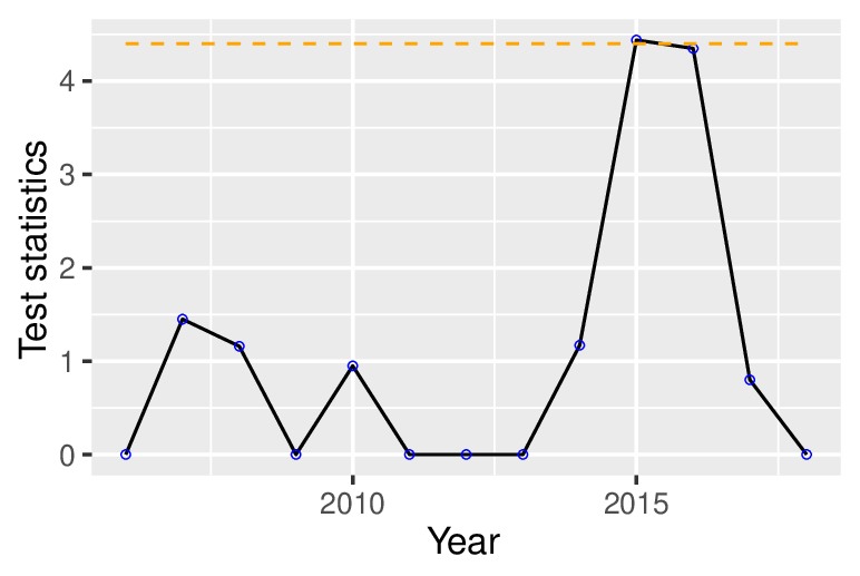
For the purpose of comparison, we also apply the benchmark methods, SSD (Yan et al., 2018), ZQ LASSO (Zou and Qiu, 2009), PCA (De Ketelaere et al., 2015) and T2(Qiu, 2013), into the gonorrhea dataset. Unfortunately, all benchmark methods are unable to raise any alarms, but our proposed SSR-tensor method raises the first hot-spot alarm in year $2016.$

Next, after the temporal detection of hot-spots, we need to further localize the hot-spots in the sense that we need to find out which state and which week may lead to the occurrence of temporal hot-spot. Because the baseline methods, SSD, ZQ-LASSO, PCA, and T2, can only realize the detection of temporal changes, we only show the localization of spatial hot-spot by SSR-Tensor, which is visualized in Figure 5.

There are some circular patterns in specific areas. For example, CENTRAL(Ark, La, Okla, Tex) tends to have a circular pattern every $11$ weeks, which is shown in Figure 5 . Besides, there are also some circular pattern for a certain state, for instance, Kansas has the bi-weekly pattern as shown in Figure 6. To validate the bi-weekly circular pattern of Kansas, we plot the time series plot of Kansas in 2016 as well as the auto-correlation function plot in Figure 5. Besides, the auto-correlation function plot in the left panel of Figure 6 serves as a baseline. It can be seen from the middle and right plot of Figure 6 that, Kansas has some bi-weekly or tri-weekly circular pattern.

References

- Beck and Teboulle, (2009) Beck, A. and Teboulle, M. (2009). A fast iterative shrinkage-thresholding algorithm for linear inverse problems. SIAM journal on imaging sciences, 2(1):183–202.
- Call and Voss, (2016) Call, M. A. and Voss, P. R. (2016). Spatio-temporal dimensions of child poverty in america, 1990–2010. Environment and Planning A, 48(1):172–191.
- Daubechies et al., (2004) Daubechies, I., Defrise, M., and De Mol, C. (2004). An iterative thresholding algorithm for linear inverse problems with a sparsity constraint. Communications on Pure and Applied Mathematics: A Journal Issued by the Courant Institute of Mathematical Sciences, 57(11):1413–1457.
- De Ketelaere et al., (2015) De Ketelaere, B., Hubert, M., and Schmitt, E. (2015). Overview of pca-based statistical process-monitoring methods for time-dependent, high-dimensional data. Journal of Quality Technology, 47(4):318–335.
- Diggle, (2013) Diggle, P. J. (2013). Statistical analysis of spatial and spatio-temporal point patterns. CRC Press.
- Elhorst, (2014) Elhorst, J. P. (2014). Spatial panel data models. In Spatial econometrics, pages 37–93. Springer.
- Friedman et al., (2010) Friedman, J., Hastie, T., and Tibshirani, R. (2010). Regularization paths for generalized linear models via coordinate descent. Journal of statistical software, 33(1):1.
- Hamilton, (1994) Hamilton, J. D. (1994). Time series analysis, volume 2. Princeton university press Princeton, NJ.
- Hannan and Quinn, (1979) Hannan, E. J. and Quinn, B. G. (1979). The determination of the order of an autoregression. Journal of the Royal Statistical Society. Series B (Methodological), pages 190–195.
- Hawkins, (1993) Hawkins, D. M. (1993). Regression adjustment for variables in multivariate quality control. Journal of Quality Technology, 25(3):170–182.
- Hu and Yuan, (2009) Hu, K. and Yuan, J. (2009). Batch process monitoring with tensor factorization. Journal of Process Control, 19(2):288–296.
- Kolda and Bader, (2009) Kolda, T. G. and Bader, B. W. (2009). Tensor decompositions and applications. SIAM review, 51(3):455–500.
- Lai and Lim, (2015) Lai, T. L. and Lim, J. (2015). Asymptotically efficient parameter estimation in hidden markov spatio-temporal random fields. Statistica Sinica, pages 403–421.
- Lan et al., (2004) Lan, H., Zhou, C., Wang, L., Zhang, H., and Li, R. (2004). Landslide hazard spatial analysis and prediction using gis in the xiaojiang watershed, yunnan, china. Engineering geology, 76(1-2):109–128.
- Lichstein et al., (2002) Lichstein, J. W., Simons, T. R., Shriner, S. A., and Franzreb, K. E. (2002). Spatial autocorrelation and autoregressive models in ecology. Ecological monographs, 72(3):445–463.
- Liu et al., (2010) Liu, J., Yuan, L., and Ye, J. (2010). An efficient algorithm for a class of fused lasso problems. In Proceedings of the 16th ACM SIGKDD international conference on Knowledge discovery and data mining, pages 323–332. ACM.
- Louwerse and Smilde, (2000) Louwerse, D. and Smilde, A. (2000). Multivariate statistical process control of batch processes based on three-way models. Chemical Engineering Science, 55(7):1225–1235.
- Qiu, (2013) Qiu, P. (2013). Introduction to statistical process control. Chapman and Hall/CRC.
- Reynolds and Madden, (1988) Reynolds, K. and Madden, L. (1988). Analysis of epidemics using spatio-temporal autocorrelation. Phytopathology, 78(2):240–246.
- Šaltytė Benth and Šaltytė, (2011) Šaltytė Benth, J. and Šaltytė, L. (2011). Spatial–temporal model for wind speed in lithuania. Journal of Applied Statistics, 38(6):1151–1168.
- Tran et al., (2012) Tran, L., Navasca, C., and Luo, J. (2012). Video detection anomaly via low-rank and sparse decompositions. In 2012 Western New York Image Processing Workshop, pages 17–20. IEEE.
- Yan et al., (2017) Yan, H., Paynabar, K., and Shi, J. (2017). Anomaly detection in images with smooth background via smooth-sparse decomposition. Technometrics, 59(1):102–114.
- Yan et al., (2018) Yan, H., Paynabar, K., and Shi, J. (2018). Real-time monitoring of high-dimensional functional data streams via spatio-temporal smooth sparse decomposition. Technometrics, 60(2):181–197.
- Zhu et al., (2005) Zhu, J., Huang, H.-C., and Wu, J. (2005). Modeling spatial-temporal binary data using markov random fields. Journal of Agricultural, Biological, and Environmental Statistics, 10(2):212.
- Zou et al., (2012) Zou, C., Ning, X., and Tsung, F. (2012). Lasso-based multivariate linear profile monitoring. Annals of Operations Research, 192(1):3–19.
- Zou and Qiu, (2009) Zou, C. and Qiu, P. (2009). Multivariate statistical process control using lasso. Journal of the American Statistical Association, 104(488):1586–1596.