Superconductor-like effects in an AC driven normal Mott-insulating quantum dot array
Abstract
We study the current response of an AC driven dissipative Mott insulator system, a normal quantum dot array, using an analytical Keldysh field theory approach. Deep in the Mott insulator regime, the nonequilibrium steady state (NESS) response resembles a resistively shunted Josephson array, with a nonequilibrium Mott insulating to conductor transition as the drive frequency is increased. The diamagnetic component of the NESS in the conducting phase is anomalous, implying negative inductance, strikingly reminiscent of the -pairing phase of a Josephson array with negative phase stiffness. However in the presence of an additional DC field the signature of supercurrent - Shapiro steps - is completely absent. We interpret these properties as number-phase fluctuation effects shared with Josephson systems rather than superconductivity.
I Introduction
The nonequilibrium response of strongly correlated quantum systems is a challenging problem requiring understanding of the many-body excitation spectra, wavefunctions, dynamical bottlenecks and dissipative processes. Driven Mott insulators are a prototypical example, exhibiting diverse phenomena that are otherwise not present in their equilibrium or linear-response regimes such as field/current driven insulator-metal transitions Sayyad et al. 2019; Nomura et al. 2015; Eckstein and Werner 2013a; Wall et al. 2011; Tsuji et al. 2008, Bloch oscillations or Wannier-Stark quantizationSankar and Tripathi 2019; Murakami and Werner 2018; Joura et al. 2015; Lee and Park 2014; Eckstein and Werner 2013b; Eckstein et al. 2010 and current enhanced diamagnetism Sow et al. 2017. A number of recent studies of optically excited Mott insulating half-filled Hubbard models have proposed a new route to superconductivity through doublon creation Peronaci et al. 2019; Li et al. 2019; Kaneko et al. 2019a; Werner et al. 2019; Fujiuchi et al. 2019; Görg et al. 2018; Coulthard et al. 2017; Ido et al. 2017; Tsuji et al. 2011; Rosch et al. 2008, possibly an exotic -pairing state Yang 1989. The evidence comes from superconductor-like properties such as effective attractive Coulomb correlations Peronaci et al. 2019; Coulthard et al. 2017; Tsuji et al. 2011, finite charge stiffness Kaneko et al. 2019b and off-diagonal long range order parameter correlations Kaneko et al. 2019b; Tindall et al. 2019; Kaneko et al. 2019a. However these half-filled Hubbard models are special since charge excitations necessarily create doublons. We therefore ask whether superconductor-like properties may still be seen in driven Mott insulators where charge excitations are not associated with doublons. Specifically, we study the current response of a dissipative Mott insulator system - an array of mesoscopic quantum dots each with a large and arbitrary number of interacting electrons - to an AC electric field quench.
We find that the NESS response deep in the Mott insulator regime has a striking resemblance with optically driven resistively shunted Josephson arrays on either side of a superconductor-insulator transition. We show that the frequency dependence of the current response has regimes of both diamagnetic and insulating behavior as the AC drive tunes the Mott insulator through a singularity separating insulator and metallic frequency dependences of the optical conductivity, indicating a nonequilibrium insulator-metal transition. However the sign of the diamagnetic response is anomalous (negative), tantamount to -phase slips in the links, analogous to the -pairing phase of Josephson arrays with negative phase stiffness. In the presence of a simultaneous DC bias, the DC characteristics exhibit Josephson-like photon-mediated tunneling in the form of current steps at bias values separated by integer multiples of drive frequency but crucially, Shapiro steps - a key signature of supercurrent - expected at integer multiples of are absent, unlike the observation in Josephson systems Lankhorst and Poccia 2016; Matsuura et al. 2008; Tinkham 2004. We propose that the similarities shared with reported optical response of Mott insulators are not on account of -pairing or AC-induced superconductivity but are a manifestation of number-phase duality effects common to both. Strong charge fluctuations, whether associated with underlying superconductivity or optical pumping, suppress quantum fluctuations of the phases.
Theoretical understanding of driven Mott insulators has received a significant impetus by developments in the Keldysh dynamical mean field theory (KDMFT) approach Murakami et al. 2019; Peronaci et al. 2018; Qin and Hofstetter 2018; Joura et al. 2015; Lee and Park 2014; Eckstein et al. 2010; Schmidt and Monien 2002, tensor network techniques Tindall et al. 2019, and analytic Bethe-ansatz Oka 2012 including the effective -symmetric descriptions Tripathi et al. 2016; Fukui and Kawakami 1998. Recently an alternate analytical large- effective Keldysh field theory approach Sankar and Tripathi 2019 has been developed based on the well-known Ambegaokar-Eckern-Schön (AES) rotor model Beloborodov et al. 2007; Ambegaokar et al. 1982 for electron transport in mesoscopic quantum dot arrays, effectively a dissipative Mott insulator system. This Keldysh formalism captures numerous nonequilibrium DC phenomena including Bloch-like oscillations and the field-driven insulator to metal transition. It also provides an analytical treatment of the approach to the NESS. Here we shall generalize this formalism for the AC response.
The rest of the paper is organized as follows. In Sec. II we introduce the Keldysh AES model for transport in a quantum dot chain, and obtain an expression for the current response functional. Sec. III is devoted to the study of the current response to a uniform AC drive. The analysis not only confirms a number of results such as odd harmonic generation, Bloch-like oscillations and effective attractive local Coulomb correlations, hitherto obtained from numerical KDMFT studies, but also reveals some aspects missed in the numerical studies, most notably the slow decay of the Bloch-like oscillations. We find striking similarities to the current response of superconductor Josephson junction arrays with effectively negative superfluid stiffness, reminiscent of an -pairing phase. To check if the superconductor-like optical response is indeed due to superconductivity in our system, we analyze in Sec. IV the current response when AC and DC driving fields are simultaneously present. Although photon mediated tunneling features, similar to superconducting Josephson arrays are also found here, the absence of Shapiro steps, a key signature of supercurrent, leads us to conclude that the properties are a manifestation of number-phase duality shared with superconductors. Sec. V contains a summary of our findings and a discussion.
II Model and formalism
Our starting point is a model Hamiltonian of a quantum dot array,
| (1) |
where
| (2) |
describes noninteracting electrons in the dots with energies for the dot,
| (3) |
represents Coulomb interaction, and
| (4) |
denotes interdot tunneling. Each dot contains a large number, of electrons that provide a dissipative fermionic bath with an approximate continuum of levels with mean spacing The large number of single-electron levels in each dots also serves as a large- parameter that provides useful simplifications leading to our final effective action (see below). In order to treat the tunneling effects correctly wrt the “bare” Hamiltonian which is interacting, one follows Altland and Simons 2010 the standard process of Hubbard-Stratonovich decoupling of the interaction, and eliminating the Hubbard-Stratonovich fluctuation potentials by gauge transformations of the fermion fields. Then following Refs. Sankar and Tripathi 2019; Altland and Simons 2010 (see also Appendix A) we go over to the Keldysh path integral formalism, with the action corresponding to our Hamiltonian put on the Keldysh time contour. Thereafter the fermionic degrees of freedom are integrated out, and the resulting fermionic determinant is expanded in increasing powers of the tunneling (only even powers survive). Terms in the effective action that are and higher get suppressed in the large- limit. Appendix A contains an outline of these steps. The physical significance of the large- approximation in suppressing higher order tunneling terms in the effective action is illustrated in Figure 1. Note that in one or few-orbital Hubbard models, the large- approximation is not available; hence, in that situation, higher order tunneling terms must be retained in the effective rotor action.
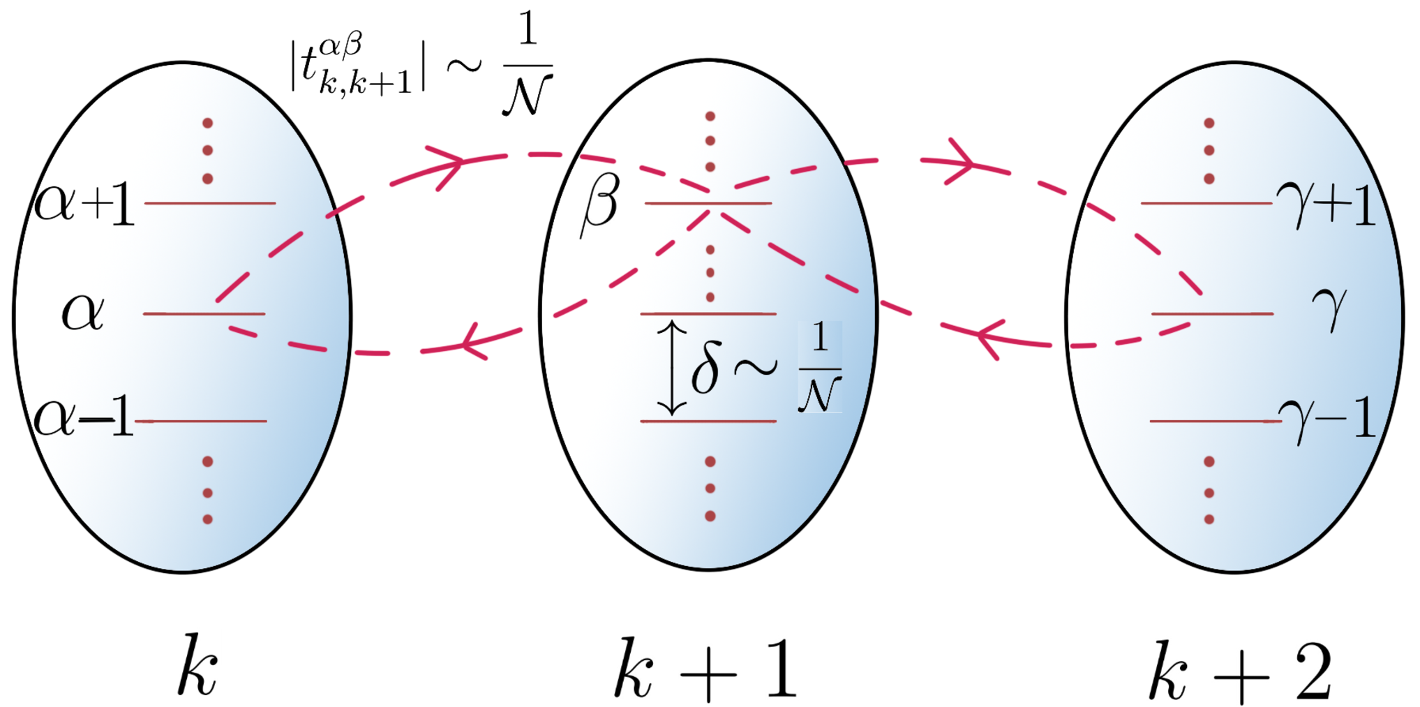
The end result is our effective Keldysh-AES rotor action,Altland and Simons 2010; Sankar and Tripathi 2019
| (5) |
for a one-dimensional array of quantum dots each with a charging energy and interdot dimensionless conductance , where
| (6) |
represents Coulomb correlations, and a nonlocal term, represents the interdot tunneling processes,
| (7) |
Here the superscripts respectively label the forward and backward parts of the Keldysh time contour, the fields in Eq. (6) are the phases dual to the charge excitations (the annihilate one charge) on the quantum dot. The phases in Eq. (7) are the difference fields across the link The kernel is a matrix in Keldysh () space with the following structureAltland and Simons 2010; Sankar and Tripathi 2019:
| (8) |
and the functions are in turn expressed in terms of products of the noninteracting local (in space) Green functions
| (9) | ||||
| (10) |
The retarded (advanced) local Green functions have the form with the th single particle energy level reckoned from the dot’s Fermi level (see Appendix A). The infintesimally small positive constant, ensures the theory has proper causal structure. Likewise, is the local Keldysh component of the noninteracting Green function, where is related to the distribution function for the single fermion excitations in a dot. Any power dissipated in the dots will result in electron heating, which would necessitate tracking the time evolution of Therefore for simplicity, we make the further assumption that the dot electrons are coupled to an external phonon bath and the electron relaxation time due to electron-phonon collisions is much shorter than that due to interdot electron tunneling, which is of the order of This allows one to replace by its equilibrium value in which case, depends only on the difference of the two time arguments Sankar and Tripathi 2019; Altland and Simons 2010. For this equilibrium case, and its Fourier transform has the simple form where is the equilibrium Fermi distribution function.
The tunneling action in Eq. (7) shares similarities with Josephson tunneling actions used to describe transport in superconducting dot arrays: both involve periodic functions of the phases necessary to ensure charge quantization, and also feature single-particle excitation gaps. Nevertheless, there are crucial differerences between the two. In Eq. (7), the kernel is nonlocal in time, unlike the Josephson case where it is local in time and has a form The time non-locality arises from integrating out the gapless particle-hole fermionic excitations in the origin and destination dots and represents the dissipative nature of the interdot tunneling process. In a JJ array, the tunneling of Cooper pairs occurs without dissipation, and particle-hole excitations are subject to the superconducting gap Another difference is that the Josephson coupling explicitly depends on the superconducting gap whereas for the normal case, the tunneling term has no characteristic energy scale. However both superconductor and normal dot chains do contain the charging term that has a characteristic scale We shall see below that the similarities of the two cases result in similar optical response, and serves to caution relying on certain optical properties for confirming superconductivity. However the differences between the two cases show up in properties such as the absence of Shapiro steps - a key signature of supercurrent - in the normal dot array.
The retarded(advanced) Green function have a causal structure, i.e., and . The same causality structure is obeyed by . Additionally, in Fourier space the following identities facilitate the calculation of expectation value of current response:
| (11) | ||||
| (12) |
where with the equilibrium Bose distribution (see Appendix A). In the rest of this paper, we choose to work in units
We introduce the external AC electric field as a time-dependent “classical” vector potential on the links, turned on at time (a quench),
| (13) |
This changes the tunneling part of the action, Eq. (7), by incorporating Peierls shifts in the phase differences, where The nonequilibrium current, in a link is obtained in the usual manner by introducing infinitesimal quantum components of the vector potential, and varying the action with respect to it.
Defining , the current functional in terms of phase fields is
| (14) |
where we have skipped the site indices for brevity. The above expression for the current response is formally exact; however the averaging over the fields gives contributions in increasing powers of the tunneling conductance, with the leading order corresponding to the atomic limit.
III Nonequilibrium AC current response
We are interested in the current response of our infinite array deep in the Mott insulator regime, where transport is dominated by sequential tunneling terms since at any order in tunneling, the cost for creating a particle-hole pair is always paid. In contrast, higher order tunneling effects are important in short arrays, or where Interdot tunneling processes also lead to the renormalization of the charging energy due to virtual tunneling to nearby dots. It is known that such processes result in corrections to which for do not make a qualitative difference to our findings except for replacing by its renormalized value Falci et al. 1995. In contrast, when the effect of the surrounding dots becomes important, and indeed, Coulomb blockade effects tend to get washed out, and the current response becomes resistive Beloborodov et al. 2007.
In the rest of our analysis, we shall compute only the leading order contribution to the current response. Figure 2 provides a pictorial illustration of why higher order tunneling effects are not significant in infinite quantum dot arrays deep in the Mott insulator regime.

Instead of working with the charging action of Eq. (6) that involves only the phases, it is convenient to work with a number-phase respresentation. For this, we rewrite the action in Eq. (6) as and decouple the first term introducing Hubbard-Stratonovich fields
| (15) |
Here is the classical (quantum) component of the charge excitation on the dot and is conjugate to At this stage, the charge variable is unconstrained. We allow for finite winding numbers in
| (16) |
where is a time scale longer than any others in the problem, and the phase on the RHS satisfies Dirichlet boundary conditions, Summing over the winding numbers forces to take only integer values. An in-depth discussion of the charge quantization emerging from such considerations can be found in the literature, for example in the textbook Ref. Altland and Simons 2010.
Performing the average with respect to the phase fields, yields the expectation value for the current. To leading order in the perturbation series, the averaging requires calculation of bare bond correlators defined as
| (17) |
where denotes averaging with the bare action. The bare bond correlator can be factorised into a product of two single site correlators:
| (18) |
where
| (19) |
and the site correlators can be shown to beSankar and Tripathi 2019
| (20) | ||||
| (21) |
The expectation value of the current response so obtained is
| (22) |
We use , and expand the exponentials containing the vector potential making use of the Jacobi-Anger formula, and perform the time integrals to obtain our final expression for following the quench:
| (23) |
Here the are Bessel functions of the first kind, and the functions Ci and si are respectively the trigonometric integrals, and We have used here the standard notation for the trigonometric integrals, the sine counterpart, of is related to through
The physical significance of the different contributions to the current in Eq. (23) may be understood as follows. The first line in Eq. (23) describes Bloch-like oscillations at a frequency The amplitude of the Bloch-like oscillations, a signature of charge quantization, falls inversely with time following the quench owing to the presence of dissipation. Such decay of Bloch oscillations is not seen in KDMFT studies of dissipationless half-filled Hubbard chains Murakami and Werner 2018, and could be a consequence of insufficiently long waiting time in the numerical simulations.
At long times, only the contributions from the last three lines of Eq. (23) survive and the NESS current is obtained by simply making the substitution,
The parameter is the number of photons required to excite an electron through the Mott gap, while controls the strength, of an -photon process. The logarithmic singularities at the thresholds are not the expected response of a gapped system but reflect the collective response of the dot electrons upon a tunneling event, similar to the X-ray edge phenomenon. The similarity with X-ray edge singularity is there because each dot has a large number of electrons and every tunneling event shifts the entire electron band by a large amount,
Figure 3 shows the transient current response following the AC quench, in four different parameter regimes. The left insets in (a)-(d) show the late time current response, together with the AC field, while the right insets show the power spectrum of as a function of frequency, measured in units of The power spectra all show a peak at and for stronger field strengths, higher harmonics appear at odd integer multiples of corresponding to multiphoton processes. The vertical dashed lines in the power spectra indicate the position of at which the Bloch-like oscillations, a signature of charge quantization, occur.

Figures 3(a), (b) correspond to where the Mott gap greatly exceeds the driving frequency. In both cases the phase of the current response is approximately ahead of the driving field, which, in combination with the insulating frequency dependence (see analysis below), resembles a capacitor. The power spectrum of the current in Fig. 3(a), where shows significant multiphoton peaks, but a distinct signature of the Bloch-like oscillations at is not evident. In contrast, the Bloch-like peak at is clearly visible in Fig. 3(b) where so that multiphoton processes that could excite electrons across the Mott gap, are suppressed. Since power dissipation is governed by the component of the current that is in phase with the driving field, both (a) and (b) correspond to weak dissipation. In Fig. 3(c), where and charge excitations induced by both single and multiphoton processes are significant. The current response is predominantly at the driving frequency, and in phase with the AC field, much like a resistor, which one would expect Oka 2012 due to pair production facilitated by the small Mott gap and large electric field strength. In Fig. 3(d), the large driving frequency implies single-photon dominated charge excitations. We show below that the frequency dependence is that of a resistively shunted inductor. Similar odd harmonic generation and multiphoton assisted tunneling phenomena have also been reported in recent KDMFT-based numerical studies Murakami et al. 2018; Murakami and Werner 2018; Eckstein et al. 2010.
We now examine the limits where the current response is capacitative or inductive. For simplicity we consider the single-photon dominated regimes where and Eq. (23) for the NESS current simplifies to ()
| (24) |
At low frequencies where the current is proportional to the derivative of the driving field - a capacitative response characteristic of a Mott insulator. At high frequencies, single-photon processes are sufficient to ensure charge excitations across the Mott gap, and the current is approximately linear-response type, having components proportional to the driving field as well as to its time integral. Apart from an additional enhancement by a factor it is essentially that of a resistively shunted inductor, with negative link inductance . While this behavior also superficially resembles that of a classical series circuit; however, the term there has a very different dependence on which is the interdot Thouless energy of diffusion of a particle-hole pair. This parameter enters our expression in a manner similar to the Josephson energy in superconductor dot arrays. The inductive response is also unrelated to the surface plasmon related Mie resonance that occurs in the same system Tripathi and Loh 2006. As the current response is resistive, and independent of Figure 4 shows the magnitude of the dominant single-photon component of the current in both these frequency limits. Kinks in curves are seen at The logarithmic non-analyticities separating insulating and metallic frequency dependence of the linear response current indicate an insulator to metal transition.

Figure 5 shows the behavior of the frequency derivative, of the single photon component of the current response as a function of the distance from the threshold This provides a clearer illustration of the frequency driven insulator to metal transition. Upon crossing the threshold the current response changes from insulating (capacitative) to metallic, which is seen in the increase and subsequent decrease of through the threshold. It is evident from the expression for the current response, Eq. 23 that the singularity in the current response at is essentially logarithmic. The collapse of the curves for different parameter values indicates a universal singular response that depends only on the dimensionless frequency

Multiphoton processes become important at low frequencies, This is evident in Fig. 3a. We found that these processes are typically much smaller than the single photon contribution. In Fig. 6 we present plots for the third harmonic (and the derivative) of the current response. The weak logarithmic singularities are present at the threshold and there is a scaling collapse at the threshold, similar to the single photon case. The three-photon contribution is smaller than the dominant single-photon contribution by a factor of around 100.


This NESS response exhibits remarkable similarities with resistively shunted Josephson arrays. The high frequency regime resembles that of a superconducting Josephson array albeit with negative stiffness, amounting to -phase slips in the links like an -pairing phase Yang 1989. This should be compared to the Ambegaokar-Baratoff relation, for the stiffness of the Josephson junction, where is the gap to quasiparticle excitations in the dots. This effect is reminiscent of the reported AC induced attractive electron interactions enhancement reported in studies of the optically excited half-filled Hubbard models Peronaci et al. 2019; Kaneko et al. 2019a; Görg et al. 2018; Coulthard et al. 2017; Li et al. 2019; Rosch et al. 2008; Ido et al. 2017; Werner et al. 2019; Tsuji et al. 2011. Various groups have subsequently also reported the formation of an -pairing state in the presence of significant doublon excitations Kaneko et al. 2019b; Tindall et al. 2019; Kaneko et al. 2019a. Note however that in our case, although the resemblance with -pairing is there, it cannot be attributed to doublon production and condensation since the equilibrium electron number in the quantum dots is arbitrary. The question of existence of supercurrent can be addressed by looking for Shapiro steps in the current response under simultaneous AC and DC bias.
IV NESS for simultaneous AC and DC bias
To probe whether there is indeed an AC induced superconducting -pairing state in our case, we analyze below the current response in the presence of a simultaneous DC field of strength for which we choose
| (25) |
The NESS current response for this case may be obtained following the same procedure outlined above for the AC response. The expression for although straightforward to obtain, is rather cumbersome, and we introduce the following additional quantitites to simplify its presentation:
and
and .
Now, introducing the quantities and
we present our final expression for the current response in the presence of a simultaneous DC and AC bias:
| (26) |
Here, are Bessel’s function of the first kind. To get the DC component, we numerically average the current over a large time interval. The DC transconductance is .
We observe jumps in the DC transconductance, at specific values of the DC potential difference across a link
| (27) |
where is an integer, like the photon-mediated tunneling steps in the characteristics of resistively shunted Josephson arrays Tinkham 2004. The role of the quasiparticle gap, in the Josephson case is taken by the Coulomb scale here. However, in contrast with the Josephson case, additional Shapiro steps that appear in intervals of and are associated with the supercurrent, are absent here. For DC transport occurs through stimulated emission of photons while for photon-assisted tunneling takes place. Figure 7 shows the DC transconductance when a simultaneous DC bias, is also applied. In the absence of the AC field, the DC transconductance is known to have a threshold behavior Matsuura et al. 2008, vanishing for and assuming the value for When the AC drive is also turned on, the threshold shifts to a lower value and transconductance is zero for where is the greatest integer less than or equal to This process is photon-assisted tunneling. When steps continue to appear in the transconductance but now they are associated with tunneling accompanied by stimulated photon emission.

V Discussion
To summarize, we showed that the current response to an AC drive in our dissipative Mott insulator chain undergoes a transition from an insulator frequency dependence at low frequencies to a conducting, diamagnetic frequency dependence for high frequencies with an effective phase stiffness the Thouless energy for interdot diffusion of a particle-hole pair. The transition occurs at the threshold for photon-assisted transition across the Mott gap. The presence of a large number of electrons in the dots results in characteristic logarithmic singularities reminiscent of X-ray edge phenomena in atomic physics. At high frequencies the sign of the diamagnetic response is negative and resembles -pairing Yang 1989 in the half-filled Hubbard chain. We argued that the -pairing like behavior in our model is not due to superconductivity but a consequence of strong charge fluctuations brought about by the nonequilibrium drive. This view is confirmed by the absence of Shapiro steps, a key signature of supercurrent, and also the fact that despite the diamagnetic behavior at high frequencies, the charge stiffness is zero.
For our analysis, we employ an analytical Keldysh field theory approach based on the Ambegaokar-Eckern-Schön rotor model for studying electronic transport in quantum dot arrays. Our technique correctly reproduces a number of known results on optically driven Hubbard chains (e.g. Bloch-like oscillations, odd harmonic generation, apparently attractive Coulomb correlations) obtained in numerical Keldysh-DMFT studies of optically excited half-filled Hubbard chains. However, in contrast with the numerical studies, we find a slow power-law decay of the Bloch-like oscillations. This could have been missed in earlier DMFT studies due to insufficient time lapse in the simulations following a quench.
Our treatment suggests that caution must be exercised in using optical properties to determine the existence of -pairing in driven Hubbard chains. An alternate physical explanation that emerges from our study is that most of the reported superconductor-like optical properties do not in fact require the existence of superconducting order, but rather are a consequence of number-phase duality effects that are common between Mott insulators and superconductors. To establish the existence of superconductivity, additional evidence such as the existence of supercurrent (through Shapiro steps or otherwise) or other direct evidence of off-diagonal long-range order is required.
Acknowledgements.
We thank S. Sankar for his valuable comments.Appendix A Derivation of the phase model
Here we sketch the steps leading from the microscopic Hamiltonian of Eq. (1) to the phase model. We first perform the Hubbard-Stratonovich decoupling of the Coulomb interaction:
| (28) | |||||
Since we are interested in the nonequilibrium response, we go over to the Keldysh action formalism, and label the fields on the forward and backward time contours respectively by superscripts and The Hubbard-Stratonovich fields cause large shifting of the entire electron energy bands during tunneling events. To eliminate these fields we perform gauge transformations on the fermion fields such that While the Hubbard-Stranotonovich fields get eliminated from the single electron energies, they clearly appear now in the interdot tunneling terms. It is convenient to perform here a basis rotation in Keldysh space so that the Green functions (see below) have the customary retarded, advanced, or Keldysh forms. To this end we introduce the “classical” () and “quantum” () components,
| (29) | |||||
| (30) | |||||
| (31) | |||||
| (32) |
The Keldysh action now takes the form,
| (33) | |||||
| (34) | |||||
| (35) |
where with Here, is related to the non interacting distribution function of electrons in the dot. If the number of dot electrons is large, then it can be shown Sankar and Tripathi 2019 that can be approximated by its equilibrium value In the frequency domain, this function is given by , where is the Fermi-Dirac distribution function. The infinitesimally small positive constant has been added for the theory to have proper causal structure.
The fermion-bilinear part of the action, can be integrated out easily. Let fermion Lagrangian density is , with
| (36) |
where
| (37) | |||||
| (38) |
The diagonal elements are the inverse retarded and advanced Green functions,
| (39) |
respectively. The interdot hopping matrix is diagonal in Keldysh space as well as in the time indices. We integrate out the fermions and get , where we express the fermionic determinant as
| (40) |
Now, to obtain the action in terms of the phase fields, we make a Taylor expansion of in increasing powers of the tunneling. The first term clearly vanishes as is diagonal in and Up to second order in we have
| (41) |
Here has the following structure in the Keldysh space,
| (42) |
where
| (43) |
We assume the matrix elements of are independent of the energy indices and further we replace the discrete summation over the energy indices by integrals, thereby, obtaining expression for in terms of . Denoting the mean square tunneling matrix connecting pairs of levels in the neighbouring sites as we obtain and given by,
| (44) |
where,
| (45) |
The functions have a causal structure like the and are given by
| (46) | |||||
| (47) |
where the Keldysh component Note that the kernel involves products of single-fermion Green functions, and thus represents a bosonic propagator. It takes a very simple form in the frequency domain.
We make use of the following identities in the frequency domain to simplify the matrix elements:
| (48) | |||
| (49) | |||
| (50) |
where and is the equilibrium Bose-Einstein distribution function. Above identities enables us to make a simplification as follows:
| (51) | |||
| (52) |
We now justify dropping the higher order tunneling terms such as in the large- approximation. Physically, the tunneling matrix elements must scale as (where is of the order of the number of conduction electrons in a dot) so that the dimensionless interdot conductance is independent of and physically meaningful. Higher order terms do not contribute in the large limit. For example, in the aforementioned fourth order term, the tunneling elements contribute an overall scaling factor of while the sum over internal indices contributes only a scaling factor of resulting in this term becoming insignificant in the large- sense. For a detailed analysis of the role of large- we refer to the arguments given in Ref. Sankar and Tripathi 2019.
References
- Sayyad et al. (2019) S. Sayyad, R. Žitko, H. U. R. Strand, P. Werner, and D. Golež, Phys. Rev. B 99, 045118 (2019).
- Nomura et al. (2015) Y. Nomura, S. Sakai, M. Capone, and R. Arita, Science Advances 1, e1500568 (2015).
- Eckstein and Werner (2013a) M. Eckstein and P. Werner, Phys. Rev. Lett. 110, 126401 (2013a).
- Wall et al. (2011) S. Wall, D. Brida, S. R. Clark, H. P. Ehrke, D. Jaksch, A. Ardavan, S. Bonora, H. Uemura, Y. Takahashi, T. Hasegawa, et al., Nature Physics 7, 114 (2011).
- Tsuji et al. (2008) N. Tsuji, T. Oka, and H. Aoki, Phys. Rev. B 78, 235124 (2008).
- Sankar and Tripathi (2019) S. Sankar and V. Tripathi, Phys. Rev. B 99, 245113 (2019).
- Murakami and Werner (2018) Y. Murakami and P. Werner, Phys. Rev. B 98, 075102 (2018).
- Joura et al. (2015) A. V. Joura, J. K. Freericks, and A. I. Lichtenstein, Phys. Rev. B 91, 245153 (2015).
- Lee and Park (2014) W.-R. Lee and K. Park, Phys. Rev. B 89, 205126 (2014).
- Eckstein and Werner (2013b) M. Eckstein and P. Werner, in Journal of Physics: Conference Series, Vol. 427 (IOP Publishing, 2013) p. 012005.
- Eckstein et al. (2010) M. Eckstein, T. Oka, and P. Werner, Phys. Rev. Lett. 105, 146404 (2010).
- Sow et al. (2017) C. Sow, S. Yonezawa, S. Kitamura, T. Oka, K. Kuroki, F. Nakamura, and Y. Maeno, Science 358, 1084 (2017).
- Peronaci et al. (2019) F. Peronaci, O. Parcollet, and M. Schiró, arXiv preprint arXiv:1904.00857 (2019).
- Li et al. (2019) J. Li, D. Golez, P. Werner, and M. Eckstein, arXiv preprint arXiv:1908.08693 (2019).
- Kaneko et al. (2019a) T. Kaneko, T. Shirakawa, S. Sorella, and S. Yunoki, Phys. Rev. Lett. 122, 077002 (2019a).
- Werner et al. (2019) P. Werner, J. Li, D. Golez, and M. Eckstein, arXiv preprint arXiv:1908.08515 (2019).
- Fujiuchi et al. (2019) R. Fujiuchi, T. Kaneko, Y. Ohta, and S. Yunoki, Phys. Rev. B 100, 045121 (2019).
- Görg et al. (2018) F. Görg, M. Messer, K. Sandholzer, G. Jotzu, R. Desbuquois, and T. Esslinger, Nature 553, 481 (2018).
- Coulthard et al. (2017) J. R. Coulthard, S. R. Clark, S. Al-Assam, A. Cavalleri, and D. Jaksch, Phys. Rev. B 96, 085104 (2017).
- Ido et al. (2017) K. Ido, T. Ohgoe, and M. Imada, Science Advances 3, e1700718 (2017).
- Tsuji et al. (2011) N. Tsuji, T. Oka, P. Werner, and H. Aoki, Phys. Rev. Lett. 106, 236401 (2011).
- Rosch et al. (2008) A. Rosch, D. Rasch, B. Binz, and M. Vojta, Phys. Rev. Lett. 101, 265301 (2008).
- Yang (1989) C. N. Yang, Phys. Rev. Lett. 63, 2144 (1989).
- Kaneko et al. (2019b) T. Kaneko, S. Yunoki, and A. J. Millis, arXiv preprint arXiv:1910.11229 (2019b).
- Tindall et al. (2019) J. Tindall, B. Buča, J. R. Coulthard, and D. Jaksch, Phys. Rev. Lett. 123, 030603 (2019).
- Lankhorst and Poccia (2016) M. Lankhorst and N. Poccia, Journal of Superconductivity and Novel Magnetism 29, 623 (2016).
- Matsuura et al. (2008) T. Matsuura, K. Inagaki, and S. Tanda, in Journal of Physics: Conference Series, Vol. 129 (IOP Publishing, 2008) p. 012024.
- Tinkham (2004) M. Tinkham, Introduction to Superconductivity (Courier Corporation, 2004).
- Murakami et al. (2019) Y. Murakami, M. Eckstein, and P. Werner, arXiv preprint arXiv:1911.04183 (2019).
- Peronaci et al. (2018) F. Peronaci, M. Schiró, and O. Parcollet, Phys. Rev. Lett. 120, 197601 (2018).
- Qin and Hofstetter (2018) T. Qin and W. Hofstetter, Phys. Rev. B 97, 125115 (2018).
- Schmidt and Monien (2002) P. Schmidt and H. Monien, eprint arXiv:cond-mat/0202046 (2002), cond-mat/0202046 .
- Oka (2012) T. Oka, Physical Review B 86, 075148 (2012).
- Tripathi et al. (2016) V. Tripathi, A. Galda, H. Barman, and V. M. Vinokur, Physical Review B 94, 041104(R) (2016).
- Fukui and Kawakami (1998) T. Fukui and N. Kawakami, Physical Review B 58, 16051 (1998).
- Beloborodov et al. (2007) I. S. Beloborodov, A. V. Lopatin, V. M. Vinokur, and K. B. Efetov, Rev. Mod. Phys. 79, 469 (2007).
- Ambegaokar et al. (1982) V. Ambegaokar, U. Eckern, and G. Schön, Phys. Rev. Lett. 48, 1745 (1982).
- Altland and Simons (2010) A. Altland and B. D. Simons, Condensed Matter Field Theory (Cambridge University Press, 2010).
- Falci et al. (1995) G. Falci, G. Schön, and G. T. Zimanyi, Phys. Rev. Lett. 74, 3257–3260 (1995).
- Murakami et al. (2018) Y. Murakami, M. Eckstein, and P. Werner, Phys. Rev. Lett. 121, 057405 (2018).
- Ben-Tal et al. (1993) N. Ben-Tal, N. Moiseyev, and A. Beswick, Journal of Physics B: Atomic, Molecular and Optical Physics 26, 3017 (1993).
- Tripathi and Loh (2006) V. Tripathi and Y. Loh, Physical Review B 73, 195113 (2006)