We study the few-body dynamics of dipolar bosons in one-dimensional double-wells. Increasing the interaction strength, by investigating one-body observables we study in the considered few-body systems tunneling oscillations, self-trapping and the regime exhibting an equilibrating behaviour. The corresponding two-body correlation dynamics exhibits a strong interplay between the interatomic correlation due to non-local nature of the repulsion and the inter-well coherence. We also study the link between the correlation dynamics and the occupation of natural orbitals of the one-body density matrix.
Quantum dynamics of few dipolar bosons in a double-well potentialJournal: Eur. Phys. J. D
1 Introduction
The study of the tunneling quantum dynamics of ultracold atoms in double-well potentials is a major tool to investigate macroscopic coherent effects and many-body properties 5. Given the very high level of manipulation and control of quantum gases, the direct observations of tunneling and nonlinear self-trapping is experimentally possible for ultracold bosons andrea1; prl95; natphy1; andrea2; Levy; prl98; nature455; LeB; contact4; Xhani19 and fermions Liscience; Lidiss; Luick; Kwon both for double- and multi-well potentials.
When in the uncoupled wells the system can be described by macroscopic wavefunctions, one has that the superfluid dynamics in the double-well potential realizes the so-called Bosonic Josepshon junction (BJJ). For a Bose-Einstein condensate in a double-well potential, interactions between the particles plays a crucial role. When the initial population imbalance of the two wells is below a critical value, Josephson oscillations are predicted 5; zapata. These two different dynamical regimes, Josephson oscillations and nonlinear self-trapping, for a BEC in a double-well potential are commonly described at the mean-field level 5; rag; st; ab; cat. To study effects of quantum fluctuations and collapse-revival, one may resort to quantum two-mode models Jav1997; Raghavan1999; Franzosi2000; smerzi2000; bosehubbard2; Giovanazzi; DellAnna; Bila. Beyond mean-field effects are very important for coupled one-dimensional systems Jo; gritsev; Aga; aPolo18; Pigneur18; Polo.
The solution of the time-dependent many-boson
Schrödinger equation sheds light to several intriguing
features, including the
role played by natural orbitals (i.e., the eigenstates of one-body density matrix) corresponding to the eigenvalues smaller than
the largest one 25; 36; s40; fischer15. The many-body tunneling dynamics in one dimensional double-well trap
with contact interactions has been also studied considering the
full crossover from weak interaction to the fermionization limit, and also attractive interactions
with prl100; contact2; manybody1; contact3; Sudip2019.
The experimental realization of dipolar gases, achieved with ultracold dipolar atoms of chromium chromium1; chromium2, dysprosium dysprosium and erbium atom erbium, further enlarged the range of phenomena that can be studied 30; 31, such as coupled one-dimensional systems with tunable dipolar interaction tang19. The non-local nature of the dipolar interaction motivated several studies having as a goal the comparison of results for the quantum dynamics with non-local interactions with the corresponding short-range findings and with recent results for quantum systems with long-range couplings vodola14; gong16; lepori16; celardo16; defenu16; lepori17; igloi18; blass18; defenu18; lerose19.
The ground state properties of ultracold trapped bosons with dipolar interactions have been studied extensively both at mean-field level and in the one-dimensional limit 39; Sinha; Citro; 35; 38; Cinti; DeP; abad1; abad2; abad3 (see more refs. in 30; 31). Properties of dipolar bosons in a double well potential were studied by mean-field blume and by the quntum two-mode model mazzarella. The many-body dynamics of bosons with non-local interaction has been recently studied in halder; Sudip2019conf, addressing the effect of a finite-range interaction on density oscillation, collapse and self-trapping and focusing on the comparison between the many-body and mean-field properties. The tunneling dynamics is studied for an interaction potential modeled as with tunable strength and half width .
In the present article we would like to address
the quantum dynamics of few dipolar bosons in a
one-
dimensional double-well. The few body systems
we are going to study have the advantage that it is possible
to investigate in detail the full one-body density matrix and correlation
functions. In this way the effect of the non-local nature of the interaction
and of the one-dimensional nature of the potential on the quantum dynamics
can be investigated in details, and the dynamical regimes determined
by them can be visualized and understood. This will give insights on the more
complicated problem of many-body dynamics of one-dimensional dipolar
atoms in double-well dynamics and their quantum tunneling effects
to characterize what are the differences and anologes with the usual
mean-field findings.
Moreover, our results will be lead us to to
make a qualitative link between the observed dynamics of quantum correlations with the interatomic and inter-well correlations. The observed tunneling
dynamics is also connected with the occupation of the natural orbitals.
The non-local, dipolar interaction is modeled as
| (1) |
( being the distance between two particles located in and ),where is the strength of dipolar interaction and is a cutoff parameter to avoid the divergence at (see the corresponding discussion in Sinha). is determined by the scattering length and transverse confinement Olshanii:98. In the follwing we keep , corresponds to repulsive dipolar bosons. We prepare the initial state with complete population imbalance in the asymmetric double-well, with all bosons stayng in the right well. The asymmetric double-well is modeled for simplicity as a superposition of three terms: a harmonic oscillator, a Gaussian with a central barrier and a linear external potential prl100. In dimensionless units reads
| (2) |
with the parameter is initally kept sufficiently large to make the right well energetically favorable. The initial state is prepared with practically all atoms in the right well. To study the dynamics in the symmetric double-well, is then instantaneously ramped down to zero at . We solve the time-dependent Schrödinger equation for dipolar bosons. The tunneling dynamics is monitored by the one-body density, the population in the right well, the population imbalance and the two-body density for various choices of . At , we observe pure Rabi oscillation Leggett. With very weak interactions, the Rabi oscillation is modified in amplitude. With larger , self-trapping is observed. When is sufficiently strong, a new regime sets in and the bosons appear to equilibrate in two wells. These four kind of dynamics are further linked with intricated interplay interatomic correlation and inter-well coherence. We observe that, for the considered number of particles, the many-body state occupies many natural orbitals in this one-dimensional setup also when is small. A marked occupation of different natural orbitals is observed for very high value of , where a vanishig population imbalance is observed for large times.
2 The model
The time-dependent many-body Schrödinger equation for interacting bosons is given by
| (3) |
(with ). Here, the Hamiltonian is given by
| (4) |
is the one-body term in the Hamiltonian, with the potential given by Eq. (2) with during the dynamics and chosen (for ) to be large to determine the initial state as described in the Introduction. is the interparticle potential, given in Eq. (1). The total Hamiltonian is written in dimensionless units, as obtained by dividing the dimensionful Hamiltonian by ( is the mass of the bosons and is an appropriately chosen length scale).
In the following Eq.(4) is solved by the numerical many-body method called multi-configuration time-dependent Hartree method for bosons (MCTDHB) Streltsov2007; Ofir2008 implemented in the MCTDH-X software x; y; axelN2; axelN3. The MCTDHB has been extensively used in different trapping potentials and interactions budha1; budha2; budha3; MCTDHB_OCT; MCTDHB_Shapiro; cao1; cao2; NJP2015Schmelcher; axelN6; Axel2017; NJP2017Camille; NJP2017Schmelcher; rhombik; rhombik2; rhombik3. MCTDH-X has been verified against experimental predictions axelprx and is reviewed in Ofir2019Rev.
The many-body wavefunction in a complete set of time-dependent permanents, distributing bosons in time-dependent single particle orbitals. Thus the ansatz for the many-body wavefunction is
| (5) |
with
| (6) |
In Eq. (5) the summation runs over all possible configurations
The (with ) are the time-dependent permanents, the operators create a boson in the th single particle state , and is the vacuum. The bosonic annihilation and corresponding creation operators obey the canonical commutation relation at any time. It is important to emphasize that in the ansatz (5) both the expansion coefficients and the orbitals that build up the permanents are time-dependent and fully variationally optimized quantities.
In the limit of , the expansion (5) is exact. However, we limit the size of the Hilbert space during our computation requiring proper convergence. As permanents are time-dependent, a given degree of accuracy is reached with a shorter expansion compared to time-independent basis. To solve the time-dependent wavefunction , we utilize the time-dependent variational principle LF1; LF2. We substitute the many-body ansatz into the functional action of the time-dependent Schrödinger equation and require the stationarity of the functional action with respect to and which lead to the working equations of the MCTDHB method Ofir2008; axelN3.


3 Results
To prepare the initial state, we propagate the equations of motion in imaginary time starting for an initial guess, so to have the ground state of interacting bosons in the right well of the asymmetric double-well given by Eq. (2) at . Chosen values of the parameters are and . To study the dynamics in the symmetric double-well we ramp down at . We consider increasing values of . We choose in our numerical simulations, as represenatives of the different regimes we observed. Throughout our work, we perform the computation with orbitals to have converged results. We observed negligible quantitative difference between the computed quantities with and orbitals. Convergence is also assured as the occupation in the last orbital is close to zero.
We observe that for the considered values , the ratio between the height of the potential, , and the chemical potential, is, respectively, . Since in general the two-mode ansatz is expected to reasonably work when , then varying we pass from a regime in which is well larger than to the one in which smaller than .
The tunneling dynamics is presented through the study of the following quantities:
(a) One-body tunneling dynamics:
From the many-body wavefunction ,
the reduced one-body density matrix is calculated as
| (7) |
Its diagonal gives the one-body density , defined as
| (8) |
It gives the density at the position and time , when the contribution of other particles is traced out.
For each choice of , we calculate till time . We present in Fig.1 for different values
of . Comparison is made with the non-interacting case. In absence of any interactions (), the atoms simply exhibit
Rabi oscillation between both wells. For (a very small value), we observe tunneling dynamics, with
the frequency and amplitude of oscillations significantly affected by the repulsive tail of non-local
interaction.
We do the computation for several other number of dipolar bosons, and observe the same dynamics.
For , the tunneling dynamics exhibits a kind of self-tapping.
The population in the right well is nearly stationary even for long time.
The self-trapping at a relatively
weak interaction appears to be a consequence of long-range repulsive tail of the dipole interaction. For contact interaction (not shown here), we find the self-trapping behaviour but for much higher interaction strength. We report also
the computation with . We observe clear signature of self-trapping at short time dynamics. However, as expected,
due to quantum fluctuations, the bosons do not remain in the self-trapped state for very long time irrespective of the particle number.
For much higher interaction strength, with , we observe equilibration dynamics. An
equal number of particles settle in the two wells.
(b) Population imbalance:
We further calculate the population in the right well using
| (9) |
and plot in Fig. 2 for the same choice of the values of . For , we again observe pure Rabi oscillations
as expected. For , as we introduce small correlations, we observe two different scale of dynamics.
Up to a time , the number of bosons in the right well fluctuates. At longer time dynamics, we observe a trend of partial equilibration,
with the value of trying to saturate at . When , which is ten times larger than the previous one,
we observe a single scale of dynamics, with remaining close to unity throughout the dynamics.
From the direct calculation of the population in the right well, we estimate that for this choice of , the self-trapping is close to 90%.
When we analyze the dynamics with , the system shows a different type of single scale dynamics i.e. equilibration.
With , we find in this state .
Thus when the strength of dipolar interaction is tuned, we observe four kinds of dynamical features: pure Rabi oscillation,
deformed Rabi oscillation with some signature of partial equilibration at large times, nonlinear self-trapping and equilibration.
We also compute the population imbalance as
| (10) |
and its average value calculated as
| (11) |
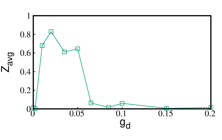

We plot as a function of in Fig. 3. It exhibits a kind of crossover between the four kind of dynamics reported above.
is zero for the two extreme cases, namely Rabi oscillation for non-interacting limit and equilibration dynamics for strong
interaction. Whereas maximum population imbalance occurs at some interaction strength which corresponds to self-trapping.
Thus the width of the curve qualitatively gives an estimate to have the interaction regime for self-trapping.
(c) Two-body correlation dynamics:
Next we calculate the time evolution of the two-body density and investigate how the effect of two-body correlation comes in
the dynamics increasing . The second order reduced density matrix is defined as
| (12) |
and the diagonal part of the two-body density is given by
| (13) |

Fig.4 - Fig.6 plot the results for the spatial two-body density for , and respectively. Non-interacting bosons tunnel independently and they are not shown. For inteacting atoms, the effect of two-body correlation is measured by the competition between the non-local interaction and the inter-well coherence. Thus the two-body correlation dynamics expected to be complicated. For larger separation (characteristic length of transverse confinement), the interaction potential varies as where , for small separation the transverse confinement induces a short range cutoff . Snapshots of two-body density for are presented in Fig. 4 for different times. At such a weak interaction, the many-body states are fully coherent, with the six bosons clustered in the right well. However, during the tunneling, we observe competition between the correlation due to non-local interaction and the inter-well coherence. With evolution of time, due to the repulsive tail in the interaction, the atoms repel each other and the atoms start to tunnel (snapshot at time ). At larger times (e.g. ), we observe four equal bright spots, two diagonal () bright spots corresponding to equal number of bosons residing in the two wells, and the other two bright spots along anti-diagonal () expressing the fact that the inter-well coherence is maintained. Thus interatomic correlation and inter-well correlations are maintained in the same scale. During the course of tunneling, we can also verify that at this later time, from Fig. 2. At laters time (e.g. ), we observe highly coherent cluster set up in the left well, showing the loss of the inter-well coherence and the prevalence of the interatomic correlations. With time evolving, we observe a rather complex competition between the interatomic correlations in either well and inter-well coherence, which results in the Rabi-like oscillations shown in Fig. 2. At longer times, we observe only two bright spots along the diagonal which again corresponds to equal population in two wells (). Comparing with the snapshot at time , which also corresponds to equal population in two wells, at time the equal population is obtained at the cost of losing inter-well coherence.
In Fig. 5, we plot the two-body density taking snapshots at different times for . In this case, the initially coherent cluster settled in the right well remains same all throughout the time which corresponds to self-trapping as shown in Fig. 2. The interatomic correlation plays the crucial role. However some faded off-diagonal patches appear which signify that exactly 100% self-trapping is not obtained. It is in good agreement with Fig. 2 which exhibits that for , about 90% self-trapping. Thus the effect of inter-well coherence is very small.
In Fig. 6, we present the two-body density for stronger interaction at different times. Initially at
we observe the strong effect of the tails of the repulsive interaction tails:
the many-body state is incoherent and diffused unlike the case reported in Fig. 4 and Fig. 5.
In Fig. 6 we observe that at time four bright spots are developed which corresponds to the equal population in the two wells.
However comparing this with the snapshot at time of Fig. 4, we can clearly identify that the bright spots are now diffused
which signifies that three bosons residing in a well feel the effect of the tails of repulsive interaction. Thus atoms are incoherent in each well.
With time, the equilibration is almost maintained, however the interatomic coherence in each well depends on time.
The equilibration dynamics for is also remarkably different as compared with the case for (Fig. 4).
At time of Fig. 4, we observe almost equal population in both wells, but absence of
inter-well coherence whereas at the same time in Fig. 6, equilibration is maintained in presence
of inter-well coherence. Thus we conclude that the observed dynamics for different choices of interaction strength
is fundamentally governed by the interplay between the interatomic correlation and inter-well coherence.
(d) Fragmentation dynamics:
In mean-field theory, one orbital is macroscopically occupied and the system is condensate. However the phenomenon
of fragmentation comes in the picture when more than one orbital is significantly occupied. In our case with particles,
we define a quantfier of the observed fragmentation in the dynamics as
| (14) |
where are the time-dependent natural occupations. Thus quantifies the contribution coming from other significant orbitals. For , and , is close to zero all throughout the time evolution. However for , even at , the system is initially fragmented which is also seen in Fig. 7 (). In a very short time, increases and reaches a constant value. Then the plateau is maintained for the rest of the time. The plateau corresponds to the equilibration dynamics when the bosons equally distributed in the two wells. In the long-time dynamics (not shown here), we observe the plateau nature is maintained. As does not increase any more, the occupation in the orbitals remain unchanged: interatomic correlation does not increase further. There is no competition any more between the inter-well coherence and interatomic correlation: thus the equilibration dynamics is maintained for very long time.


4 Conclusion
We studied the few-body quantum dynamics of few dipolar bosons in a symmetric double-well. We studied Rabi oscillations in the non-interacting limit and self-trapping and finally equilibration dynamics for strong interaction. The complete dynamics for different choices of the interaction strength is presented through the one-body tunneling dynamics. We further considered the average population imbalance in the two wells as the figure of merit of the tunneling dynamics. The structure in the average population imbalance qualitatively describe the range of interaction strength to have self-trapping, as seen in Fig. 3. We observed the very interesting dynamics in the two-body density and established the link between the tunneling dynamics and the role played by the interatomic correlation and inter-well coherence. The most subtle dynamics is observed at the strong interaction strength when the many-body dynamics exhibits equilibration. Finally we observed that for equilibration dynamics, the many-body state is initially fragmented and then exhibits a plateau structure in the long time dynamics.
Several open questions are suggested by the results presented in this paper. The few-body quantum dynamics gives insights on the phases emerging from the combined presence of the non-local dipolar interaction and of the one-dimensionality. Nevertheless, a full study of the quantum dynamics of dipolar long-range atoms in one-dimensional double-well and the corresponding diagram of dynamical regimes remain to be explores, and one has to see how many-body effects in one-dimension modify the regimes holding for the few-body cases we examined. In partcular, it would be important to address how the non-local nature of the interaction modifies the corresponding results for atoms with short-range interactions in one-dimensional double-well setups. Moreover, since for very large values of , dipolar gases exhibits crystallization (see e.g. macri2; sangita), the double-well dynamics in this regime would be interesting to study. We also mention that in the standard quantum two-mode model one can rewrite the density-density interaction term between the populations of different wells in terms of the local interaction term: therefore, for high barriers, one could ask whether the tunneling dynamics in double-well potentials can be written in terms of an effective contact interaction and how the possibility of performing such a mapping depends on the dimensionality of the systems. We finally mention that the study of the quantum dynamics in presence of both non-local or dipolar and contact interactions in double-well potentials is also to a deserving subject of future investigation.
Acknowledgements.
R. Roy acknowledges the University Grant Commission (UGC) India for the financial support as a senior research fellow. B. Chakrabarti acknowledges ICTP support where major portion of the work was done.References
- (1) A. Smerzi, S. Fantoni, S. Giovanazzi, and S. R. Shenoy, Phys. Rev. Lett. 79, 4950 (1997).
- (2) F. S. Cataliotti, S. Burger, C. Fort, P. Maddaloni, F. Minardi, A. Trombettoni, A. Smerzi, and M. Inguscio, Science 293, 483 (2001).
- (3) M. Albiez, R. Gati, J. Fölling, S. Hunsmann, M. Cristiani, and M. K. Oberthaler, Phys. Rev. Lett. 95, 010402 (2005).
- (4) T. Schumm, S. Hofferberth, L. M. Andersson, S. Wildermuth, S. Groth, I. Bar-Joseph, J. Schmiedmayer, and P. Krüger, Nature Phys., 1, 57 (2005).
- (5) T. Anker, M. Albiez, R. Gati, S. Hunsmann, B. Eiermann, A. Trombettoni, and M. K. Oberthaler, Phys. Rev. Lett. 94, 020403 (2005).
- (6) S. Levy, E. Lahoud, I. Shomroni, and J. Steinhauer, Nature 449, 579 (2007).
- (7) B. V. Hall, S. Whitlock, R. Anderson, P. Hannaford, and A. I. Sidorov, Phys. Rev. Lett. 98, 030402 (2007).
- (8) J. Estève, C. Gross, A. Weller, S. Giovanazzi and M. K. Oberthaler, Nature 455, 1216 (2008).
- (9) L. J. LeBlanc, A. B. Bardon, J. McKeever, M. H. T. Extavour, D. Jervis, J. H. Thywissen, F. Piazza, and A. Smerzi, Phys. Rev. Lett. 106, 025302 (2011).
- (10) G. Spagnolli, G. Semeghini, L. Masi, G. Ferioli, A. Trenkwalder, S. Coop, M. Landini, L. Pezzé, G. Modugno, M. Inguscio, A. Smerzi, and M. Fattori, Phys. Rev. Lett. 118, 230403 (2017).
- (11)
K. Xhani, E. Neri, L. Galantucci, F. Scazza, A. Burchianti, K.-L. Lee, C. F. Barenghi, A. Trombettoni,
M. Inguscio, M. Zaccanti, G. Roati, and N. P. Proukakis,
arXiv:1905.08893 - (12) G. Valtolina, A. Burchianti, A. Amico, E. Neri, K. Xhani, J. A. Seman, A. Trombettoni, A. Smerzi, M. Zaccanti, M. Inguscio, and G. Roati, Science 350, 1505 (2015).
- (13) A. Burchianti, F. Scazza, A. Amico, G. Valtolina, J. A. Seman, C. Fort, M. Zaccanti, M. Inguscio, and G. Roati, Phys. Rev. Lett. 120, 025302 (2018).
- (14)
N. Luick, L. Sobirey, M. Bohlen, V. P. Singh, L. Mathey, T. Lompe, and H. Moritz,
arXiv:1908.09776 - (15)
W. J. Kwon, G. Del Pace, R. Panza, M. Inguscio, W. Zwerger, M. Zaccanti, F. Scazza, and G. Roati,
arXiv:1908.09696 - (16) I. Zapata, F. Sols, and A. J. Leggett, Phys. Rev. A 57, R28 (1998).
- (17) S. Raghavan, A. Smerzi, S. Fantoni, and S. R. Shenoy, Phys. Rev. A 59, 620 (1999).
- (18) A. Smerzi and A. Trombettoni, Phys. Rev. A 68, 023613 (2003).
- (19) D. Ananikian and T. Bergeman, Phys. Rev. A 73, 013604 (2006).
- (20) D. M. Jezek, P. Capuzzi, and H. M. Cataldo, Phys. Rev. A 87, 053625 (2013).
- (21) J. Javanainen and M. Wilkens, Phys. Rev. Lett. 78, 4675 (1997).
- (22) S. Raghavan, A. Smerzi, and V. M. Kenkre, Phys. Rev. A 60, R1787(R) (1999).
- (23) R. Franzosi, V. Penna, and R. Zecchina, Int. J. Mod. Phys. B 14, 943 (2000).
- (24) A. Smerzi and S. Raghavan, Phys. Rev. A 61, 063601 (2000).
- (25) R. Gati and M. K. Oberthaler, J. Phys. B 40, R61 (2007).
- (26) S. Giovanazzi, Estéve, and M. K. Oberthaler, New J. Phys. 10, 045009 (2008).
- (27) L. Dell’Anna, Phys. Rev. A 85, 053608 (2012).
- (28) M. Bilardello, A. Trombettoni, and A. Bassi, Phys. Rev. A 95, 032134 (2017).
- (29) G.-B. Jo, Y. Shin, S. Will, T. A. Pasquini, M. Saba, W. Ketterle, D. E. Pritchard, M. Vengalattore, and M. Prentiss, Phys. Rev. Lett. 98, 030407 (2007).
- (30) V. Gritsev, A. Polkovnikov, and E. Demler, Phys. Rev. B 75, 174511 (2007).
- (31) K. Agarwal, E. G. Dalla Torre, J. Schmiedmayer, and E. Demler, Phys. Rev. B 95, 195157 (2017).
- (32) J. Polo, V. Ahufinger, F. W. J. Hekking, and A. Minguzzi, Phys. Rev. Lett. 121, 090404 (2018).
- (33) M. Pigneur, T. Berrada, M. Bonneau, T. Schumm, E. Demler, and J. Schmiedmayer, Phys. Rev. Lett. 120, 173601 (2018).
- (34) J. Polo, R. Dubessy, P. Pedri, H. Perrin, and A. Minguzzi, Phys. Rev. Lett. 123, 195301 (2019).
- (35) A. I. Streltsov, O. E. Alon, and L. S. Cederbaum, Phys. Rev. A 73, 063626 (2006).
- (36) A. I. Streltsov, Phys. Rev. A 88, 041602(R) (2013).
- (37) O. I. Streltsov, O. E. Alon, L. S. Cederbaum, and A. I. Streltsov, Phys. Rev. A 89, 061602(R) (2014).
- (38) U. R. Fischer, A. U. J. Lode and B. Chatterjee, Phys. Rev.A 91, 063621 (2015).
- (39) S. Zöllner, H. Meyer, and P. Schmelcher, Phys. Rev. Lett. 100, 040401 (2008).
- (40) K. Sakmann, A. I. Streltsov, O. E. Alon and L. S. Cederbaum, Phys. Rev. Lett. 103, 220601 (2009).
- (41) K. Sakmann, A. I. Streltsov, O. E. Alon and L. S. Cederbaum,Phys. Rev. A 82, 013620 (2010).
- (42) K. Sakmann, A. I. Streltsov, O. E. Alon and L. S. Cederbaum,Phys. Rev. A 89, 023602 (2014).
- (43) S. K. Haldar and O. E. Alon, New J. Phys. 21, 103037 (2019).
- (44) A. Griesmaier, J. Werner, S. Hensler, J. Stuhler, and T. Pfau, Phys. Rev. Lett. 94, 160401 (2005).
- (45) Q. Beaufils, R. Chicireanu, T. Zanon, B. Laburthe-Tolra, E. Marchal, L. Vernac, J.-C. Keller, and O. Gorceix, Phys. Rev. A 77, 061601 (2008).
- (46) M. Lu, N. Q. Burdick, S. H. Youn, and B. L. Lev, Phys. Rev. Lett. 107, 190401 (2011).
- (47) K. Aikawa, A. Frisch, M. Mark, S. Baier, A. Rietzler, R. Grimm, and F. Ferlaino, Phys. Rev. Lett. 108, 210401 (2012).
- (48) M. A. Baranov, Phys. Rep. 464, 71 (2008).
- (49) T. Lahaye, C Menotti, L Santos, M Lewenstein and T Pfau, Rep. Prog. Phys. 72, 126401 (2009).
- (50) Y. Tang, W. Kao, K.-Y. Li, S. Seo, K. Mallayya, M. Rigol, S. Gopalakrishnan, and B. Lev, Phys. Rev. X 8, 021030 (2018).
- (51) D. Vodola, L. Lepori, E. Ercolessi, A. V. Gorshkov, and G. Pupillo, Phys. Rev. Lett. 113, 156402 (2014).
- (52) Z.-X. Gong, M. F. Maghrebi, A. Hu, M. Foss-Feig, P. Richerme, C. Monroe, and A. V. Gorshkov, Phys. Rev. B 93, 205115 (2016).
- (53) L. Lepori, D. Vodola, G. Pupillo, G. Gori, and A. Trombettoni, Ann. Physics 374, 35 (2016).
- (54) G. L. Celardo, R. Kaiser, and F. Borgonovi, Phys. Rev. B 94, 144206 (2016).
- (55) N. Defenu, A. Trombettoni, and S. Ruffo, Phys. Rev. B 94, 224411 (2016); ibid. Phys. Rev. B 96, 104432 (2017).
- (56) L. Lepori, A. Trombettoni, and D. Vodola, J. Stat. Mech. 033102 (2017).
- (57) F. Iglói, B. Bla, G. Roósz, and H. Rieger, Phys. Rev. B 98, 184415 (2018).
- (58) B. Bla, H. Rieger, G. Roósz, and F. Iglói, Phys. Rev. Lett. 121, 095301 (2018).
- (59) N. Defenu, T. Enss, M. Kastner, and G. Morigi, Phys. Rev. Lett. 121, 240403 (2018).
- (60) L. Lerose, B. Zunkovic, A. Silva, and A. Gambassi, Phys. Rev. B 99, 121112 (2019).
- (61) L. Santos, G. V. Shlyapnikov, P. Zoller and M. Lewenstein, Phys. Rev. Lett. 85, 1791 (2000).
- (62) S. Sinha and L. Santos, Phys. Rev. Lett. 99, 140406 (2007).
- (63) R. Citro, E. Orignac, S. De Palo, and M.-L. Chiofalo, Phys. Rev. A 75, 051602 (2007).
- (64) P. Bader and U. R. Fischer, Phys. Rev. Lett. 103, 060402 (2009).
- (65) N. Henkel, F. Cinti, P. Jain, G. Pupillo and T. Pohl, Phys. Rev. Lett. 108, 265301 (2012).
- (66) F. Cinti, T. Macrì, W. Lechner, G. Pupillo, and T. Pohl, Nature Communications 5, 3235 (2014).
- (67) S. De Palo, R. Citro, and E. Orignac, Phys. Rev. B 101, 045102 (2020).
- (68) M. Abad, M. Guilleumas, R. Mayol, M. Pi, and D. M. Jezek, Phys. Rev. A 84, 035601 (2011).
- (69) M. Abad, M. Guilleumas, R. Mayol, M. Pi and D. M. Jezek, Euro. Phys. Lett., 94 10004 (2011).
- (70) A. Gallem, M. Guilleumas, R. Mayol, and A. Sanpera, Phys. Rev. A 88, 063645 (2013).
- (71) M. Asad-uz-Zaman and D. Blume, Phys. Rev. A 80, 053622 (2009).
- (72) G. Mazzarella and L. Dell’Anna, EPJ ST 217, 197 (2013).
- (73) S. K. Haldar and O. E. Alon, Chem. Phys. 509, 72 (2018).
- (74) S. K. Haldar and O. E. Alon, J. Phys.: Conf. Series 1206, 012010 (2019).
- (75) M. Olshanii, Phys. Rev. Lett. 81, 938 (1998).
- (76) A. J. Leggett, Rev. Mod. Phys. 73, 307 (2001).
- (77) A. I. Streltsov, O. E. Alon, and L. S. Cederbaum, Phys. Rev. Lett. 99, 030402 (2007).
- (78) O. E. Alon, A. I. Streltsov, and L. S. Cederbaum, Phys. Rev. A 77, 033613 (2008).
- (79) E. Fasshauer and A. U. J. Lode, Phys. Rev. A 93, 033635 (2016).
- (80) Rui Lin et. al. Quantum Sci. Technol. 5 024004 (2020).
- (81) A. U. J. Lode, M. C. Tsatsos, E. Fasshauer, R. Lin, L. Papariello, P. Molignini, C. Lévêque, and S. E. Weiner, MCTDH-X:The time-dependent multiconfigurational Hartree for indistinguishable particles software, http://ultracold.org (2018).
- (82) A. U. J. Lode, Phys. Rev. A 93, 063601 (2016).
- (83) B. Chatterjee, C. Lévêque, J. Schmiedmayer, and A. U. J. Lode Phys. Rev. Lett. 125, 093602 (2020).
- (84) Budhaditya Chatterjee and Axel U. J. Lode Phys. Rev. A 98, 053624 (2018).
- (85) Budhaditya Chatterjee et. al., New J. Phys. 21, 033030 (2019).
- (86) J. Grond, J. Schmiedmayer, and U. Hohenester, Phys. Rev. A 79, 021603(R) (2009).
- (87) J. Grond, T. Betz, U. Hohenester, N. J. Mauser, J. Schmiedmayer, and T. Schumm, New J. Phys. 13, 065026 (2011).
- (88) L. Cao, S. Krönke, O. Vendrell, and P. Schmelcher, J. Chem. Phys. 139, 134103 (2013).
- (89) R. Schmitz, S. Krönke, L. Cao, and P. Schmelcher, Phys. Rev. A 88, 043601 (2013).
- (90) J. M. Schurer, A. Negretti, and P. Schmelcher, New J. Phys. 17, 083024 (2015).
- (91) A. U. J. Lode, B. Chakrabarti, and V. K. B. Kota, Phys. Rev. A 92, 033622 (2015).
- (92) A. U. J. Lode and C. Bruder, Phys. Rev. Lett. 118, 013603 (2017).
- (93) C. Lévêque and L. B. Madsen, New J. Phys. 19, 043007 (2017).
- (94) G. C. Katsimiga, S. I. Mistakidis, G. M. Koutentakis, P. G. Kevrekidis, and P. Schmelcher, New J. Phys. 19, 123012 (2017).
- (95) R. Roy, A. Gammal, M. C. Tsatsos, B. Chatterjee, B. Chakrabarti, and A. U. J. Lode, Phys. Rev. A 97, 043625 (2018).
- (96) R. Roy, C. Lévêque, A. U. J. Lode, A. Gammal, and B. Chakrabarti, Quantum Reports 1, 304 (2019).
- (97) S. Bera, R. Roy, A. Gammal, B. Chakrabarti, and B. Chatterjee, J. Phys. B 52, 21 (2019).
- (98) J.H.V. Nguyen, M.C. Tsatsos, D. Luo, A.U.J. Lode, G.D. Telles, V.S. Bagnato, and R.G. Hulet Phys. Rev. X 9, 011052 (2019).
- (99) A. Lode, C. Lévêque, L. Madsen, A. Streltsov, and O. E. Alon, rev. Mod. Phys., 92 011001 (2020).
- (100) P. Kramer and M. Saracento, Geometry of the time-dependent variational principle (Springer, Berlin, 1981).
- (101) H.-J. Kull and D. Pfirsch, Phys. Rev. E 61, 5940 (2000).
- (102) T. Macrì, F. Maucher, F. Cinti, and T. Pohl, Phys. Rev. A 87, 061602(R) (2013).
- (103) S. Bera, B. Chakrabarti, A. Gammal, M. C. Tsatsos, M. L. Lekala, B. Chatterjee, C. Lévêque, and A. U. J. Lode, Sci. Rep. 9, 17873 (2019).