A Sparsity Inducing Nuclear-Norm Estimator (SpINNEr) for Matrix-Variate Regression in Brain Connectivity Analysis
Abstract
Classical scalar-response regression methods treat covariates as a vector and estimate a corresponding vector of regression coefficients. In medical applications, however, regressors are often in a form of multi-dimensional arrays. For example, one may be interested in using MRI imaging to identify which brain regions are associated with a health outcome. Vectorizing the two-dimensional image arrays is an unsatisfactory approach since it destroys the inherent spatial structure of the images and can be computationally challenging. We present an alternative approach—regularized matrix regression—where the matrix of regression coefficients is defined as a solution to the specific optimization problem. The method, called SParsity Inducing Nuclear Norm EstimatoR (SpINNEr), simultaneously imposes two penalty types on the regression coefficient matrix—the nuclear norm and the lasso norm—to encourage a low rank matrix solution that also has entry-wise sparsity. A specific implementation of the alternating direction method of multipliers (ADMM) is used to build a fast and efficient numerical solver. Our simulations show that SpINNEr outperforms others methods in estimation accuracy when the response-related entries (representing the brain’s functional connectivity) are arranged in well-connected communities. SpINNEr is applied to investigate associations between HIV-related outcomes and functional connectivity in the human brain.
Keywords: Nuclear plus L1 norm, Low-rank and sparse matrix, Spectral regularization, Penalized matrix regression, Clusters in brain network
1 Introduction
Regression problems where the response is a scalar and the predictors constitute a multidimensional array arise often in medical applications where a matrix or a high dimensional array of measurements is collected for each subject. For example, it is of clinical interest to understand associations between: (a) alcoholism and the electrical activity of different brain regions over time collected from electroencephalography (EEG) (Li et al., 2010); (b) cognitive function and three-dimensional white-matter structure data collected from diffusion tensor imaging (DTI) (Goldsmith et al., 2014) for patients with multiple sclerosis (MS); and (c) cognitive impairment and brain’s metabolic activity data collected from three-dimensional positron emission tomography (PET) imaging (Wang et al., 2014). Our work focuses on the problem of identifying brain network connections that are associated with neurocognitive measures for HIV-infected individuals. The outcome (response) is a continuous variable and the predictors are matrix representations of functional connectivity between the brain’s cortical regions.
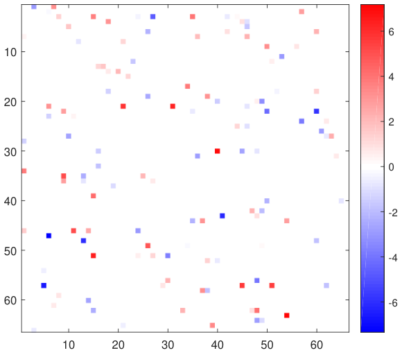
Biophysical considerations motivate our interest in estimating a matrix of regression coefficients that has the following two properties: (i) it should be relatively sparse, since we aim to identify connections that most strongly predict the outcome; and more importantly, (ii) the response-related connections form clusters, since brain activity networks are known to consist of densely connected regions. These two properties translate to the coefficient matrix having relatively small clusters, or blocks of nonzero entries, which implies that it is low-rank. Hence, we aim to solve the matrix regression problem by estimating a coefficient matrix that is both sparse and low-rank. To further illustrate our approach, consider the three matrices in Figure 1. The one in the left panel is sparse, but full-rank, the one on the right panel is low-rank, but not sparse, while the one in the middle panel is both low-rank and sparse, which is the structure we are interested in. To find such a solution, we propose a regularization method called SParsity Inducing Nuclear Norm EstimatoR (SpINNEr).


Several regularization methods have been proposed for regression problems where the response is a scalar and the predictors constitute a multidimensional array or tensor. These methods fall mainly along two investigative directions. The first treats the multidimensional array of predictors as functional data. Among the early efforts, Reiss and Ogden, 2010 extended their functional principal component regression method for one-dimensional signal predictors (Reiss and Ogden, 2007) to two-dimensional image predictors. Their method is based on B-splines with a penalty on the roughness of the coefficient function which encourages local structure but does not impose constraints on rank or sparsity. Wang et al., 2014 developed a regularized wavelet-based approach that induces sparsity in the coefficient function. The second line of research treats images as tensors rather than as functional data. Zhou et al., 2013 proposed a tensor regression framework that achieves dimension reduction through fixed-rank tensor decomposition (Kolda and Bader, 2009). They obtain the estimates by a regularized maximum likelihood approach. For regression problems with matrix covariates, Zhou and Li, 2014 proposed spectral regularization where the penalty term is a function of the coefficient matrix singular values. Using -norm of the singular values as penalty gives rise to a nuclear norm regression which induces a low-rank structure on the coefficient matrix. Our work builds upon Zhou and Li, 2014 by inducing sparsity of the coefficient matrix in terms of both its rank (low-rank) and the number of its nonzero entries (sparse). Under a Bayesian framework, Goldsmith et al., 2014 used a prior distribution on latent binary indicators to induce sparsity and spatial contiguity of relevant image locations, and appealed to Gaussian Markov random field to induce smoothness in the coefficients.
The approaches summarized above are insufficient for finding a coefficient matrix that is both sparse and low-rank. More specifically, for regularization approaches based on functional regression, Reiss and Ogden, 2010 do not impose conditions on sparsity rank, while Wang et al., 2014 do not impose any constraint on rank. For approaches based on tensor decomposition, the method of Zhou et al., 2013 can potentially induce sparsity via regularized maximum-likelihood, but the rank of the solution must be pre-specified and fixed prior to model fitting. In other words, the rank is not determined in a data-driven manner. Zhou and Li, 2014 lifted the fixed-rank constraint by using a nuclear norm—a convex relaxation of rank—as penalty, but the solution may not be sparse. Finally, Goldsmith et al., 2014 impose sparsity and spatial smoothness, which implicitly reduces complexity (and possibly rank), but this approach assumes spatially adjacent regions are similarly associated with the response.
In contrast to all of these methods, SpINNEr combines a nuclear-norm penalty with an -norm penalty that simultaneously imposes low-rank and sparsity on the coefficient matrix. Specifically, the low-rank constraint induces accurate estimation of coefficients inside response-related blocks, while outside of these blocks the sparsity constraint encourages zeros. These blocks, however, are not presumed to consist of only spatially adjacent brain regions and so this sparse-and-low-rank approach is more flexible and physiologically meaningful.
While SpINNEr seeks a singly regression coefficient matrix that is both sparse and low-rank, others have proposed estimating two structures: one low-rank and one sparse. For graphical models, in particular, Chandrasekaran et al., 2012 proposed a method for estimating a precision matrix that decomposes into the sum of a sparse matrix and a low-rank matrix when there are latent variables. Their estimation is based on regularized maximum likelihood where sparsity is induced by the -norm and low-rank is induced by the nuclear norm. Building upon Chandrasekaran et al., 2012, Ciccone et al., 2019 imposed the additional constraint that the sample covariance matrix of the observed variables is close to the true covariance in terms of Kullback-Leibler divergence, and proposed a computational solution based on the alternating direction method of multipliers (ADMM) algorithm. While Chandrasekaran et al., 2012 and Ciccone et al., 2019 assume observations to be i.i.d., Foti et al., 2016 extended the “sparse plus low-rank” framework to graphical models with time series data, whereas Basu et al., 2018 considered vector autoregressive models and directly imposed the decomposition on the transition matrix. In the matrix completion literature, the “sparse plus low-rank” decomposition has also been exploited for algorithmic concerns, enabling more efficient storage and computation Mazumder et al., 2010; Hastie et al., 2015. Our work is distinct from these proposals in that we obtain a single matrix that is simultaneously sparse and low-rank by imposing two penalties on the same matrix, rather than separately penalizing two components of a matrix.
The rest of the article is organized as follows. Section 2 further motivates and describes the objective of finding response-related clusters and translate it to a problem of finding a low-rank and sparse coefficient matrix. Section 3 formulates the objective as an optimization problem, characterizes properties of its solution, and develops an algorithm for numerical implementation. Simulation experiments are summarized in Section 4 and an application to brain imaging data is described in Section 5. We conclude with discussion in Section 6. Technical derivations of the algorithm are presented in the Appendix.
2 Clusters recovery problem
2.1 Statistical model
Assume we observe a real-valued response, , and a matrix, , for each subject, . We additionally assume a vector of covariates, , such that the matrix, , with rows , for each subject, has independent columns (hence ).
Motivated by brain imaging applications, is viewed as an adjacency matrix of connectivity information (structural or functional), each corresponds to a vector of demographic covariates and an intercept (i.e., the first entry of is 1). Additionally, we assume that there exists an (unknown) matrix and (unknown) vector whose entries represent coefficients to be estimated in the regression equation
| (2.1) |
where is the Frobenius inner product and . Unless is unusually large (greater than ), this is an informal statement of the problem which does not have a unique solution for and without further constraints. The focus of this work is on the rigorous implementation of constraints that lead to a biologically meaningful regression model having a unique solution.
We will use the equivalent graph description of the problem to build the intuition behind the assumed model (2.1). In that interpretation, brain regions are viewed as nodes in a graph and the connectivity information of th subject for these regions is represented by a matrix with zeros on the diagonal. The off-diagonal entries, , of denote weights of connectivity between regions and ; positive as well as negative weights are acceptable. If is positive, its value indicates how strongly regions and are connected, while the magnitude of negative entry indicates the level of dissimilarity. In (2.1), denotes the (unknown) matrix of regression coefficients whose entry, , represents the association between the response variable and the connectivity across regions and . We assume is symmetric and note that its diagonal entries are not included in the model, since each connectivity matrix has zeros on the diagonal. The main goal, therefore, is to estimate the off-diagonal entries of in a manner that reveals brain subnetwork structure that is associated with the response. This structure is revealed by the clusters and hubs defined by the non-zero entries in , an estimate of .
2.2 Response-related clusters
We are interested in identifying only significant brain-region connectivities and therefore we want to encourage the estimate, , to be sparse entry-wise. However, our most important goal is to protect the structure of response-related connectivities (i.e., the non-zero entries of ). Indeed, brain networks exhibit a so-called “rich club” organization, meaning that there are relatively small groups of densely connected nodes (van den Heuvel and Sporns, 2011; Zhao et al., 2019). Recent studies have demonstrated that such hubs play an important role in information integration between different parts of the network (van den Heuvel and Sporns, 2011). This structure would be lost if the process of estimating only focused on sparsity. Thus, we want the estimation process to allow for a potentially cluster-structured form of so that it may more accurately reflect the association between brain connectivities and a phenotypic outcome. However, estimating using a two-step process would imply that we must detect individual response-impacting edges prior to forming clusters from the selected edges. Clearly some cluster-defining edges and/or hubs may be missed by this preliminary focus on sparsity.
As an illustration, consider a setting where there are many response-related connectivities between a few, say , brain regions. Even if some of these effects are moderate, it is the entire cluster of regions that, as a whole, affects the response. However, if there are connections in the cluster and only the strongest effects survive a sparsity-inducing lasso estimate (Tibshirani, 1996) or other entry-wise thresholding techniques, then the “systems level” information is lost and inferring relevant information about the clusters may become impossible.
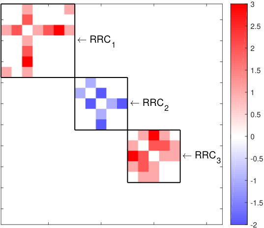
In our work, we introduce the notion of response-related clusters and focus on their selection rather than on accurate estimation of each individual effect which, in fact, would be impossible due to the limited sample size. Precisely, we define a set of nodes, , to be a response-related cluster (RRC) if for any two distinct indices there is a path of edges from connecting and , namely the sequence of the elements such as , and for . We define to be a positive response-related cluster if for every pair of its elements, and , it holds that (zeros are acceptable). Accordingly, is a negative response-related cluster if for all its elements. Motivated by the rich-club pattern of brain connectivity, we will assume that relatively few clusters of brain nodes spanning the subnetworks are strongly associated with . If the brain regions are arranged in a cluster-by-cluster ordering, this assumption is simply reflected in a block-diagonal pattern of the matrix of regression coefficients, , with blocks corresponding to RRCs (Figure 2(a) ).

2.3 A marriage of sparsity and low rank
As observed previously, most often we do not have a large enough set of samples to accurately estimate all entries of . More precisely, suppose that we are considering the MLE of under the model (2.1), without any constraints imposed on the estimates. This leads to the problem of minimizing with respect to the by matrix (we exclude and for clarity). Such a problem does not have a unique solution unless we assume that all vectors are linearly independent, implying that . If , which is rather a small number of regions compared to brain parcellations widely used in applications, this would necessitate observing data on at least subjects. Of course we can limit the degrees of freedom by assuming (very reasonably) that is symmetric but this still requires . We can reduce this number further by assuming there exist relatively few RRCs, so that is sparse (Figure 2(a) ). Let and denote the number and the average size of RRCs, respectively. However, even with an oracle telling us precisely the locations of non-zeros and we restrict the estimation to these corresponding entries of ) there are still observations required since we have, roughly, entries to estimate (and this is the simplest scenario with all clusters having the same number of nodes).
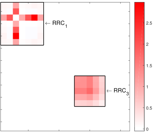
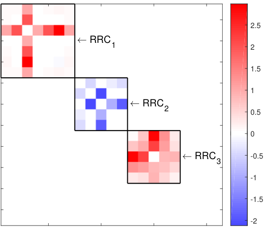
Again consider a signal with a block pattern as in Figure 2(a). For such matrices, the first a few eigenvectors (i.e., those corresponding to the largest eigenvalues) are of a special form. Assuming that they are unique (up to a change in sign), each of them may have its non-zeros located inside exactly one RRC. In our example (presented in Figure 2), the eigenvector , corresponding to the largest eigenvalue , has all its non-zeros located inside RRC3. Moreover, as a direct consequence of Perron-Frobenius theorem (Frobenius, 1912) for irreducible matrices, all coefficients of located inside RRC3 must be either strictly positive or strictly negative. That is, the non-zero entries of coincide precisely with the indices of RRC3 and the matrix (i.e., the best rank-one approximation of ) and corresponds to the entire corresponding block in Figure 2(e). In fact, the first several, say , eigenvectors may effectively summarize the structure of signal via the best rank- approximation, , of (Figure 2(g)).
Returning to the calculations, if we restrict attention to the general structure of reflected by its first eigenvectors and assume that each of them has roughly non-zeros within one of the RRCs, then we obtain , namely , coefficients to estimate (according to an oracle). This refocus on “structured sparsity” not only reduces the computational requirements, but also adds to the physiological interpretation.
In summary, we propose a method called SParsity Inducing Nuclear Norm EstimatoR (SpINNEr) that constructs a low-rank and sparse estimate of under the model (2.1). It provides a principled approach to estimating via: (i) exploiting its dominant eigenvectors to accurately estimate block-structured coefficients and, simultaneously, (ii) imposing sparsity outside of these blocks.
3 Methodology
3.1 Penalized optimization
With the goal of encouraging a regression coefficient (matrix) estimate to be both sparse and low-rank, SpINNEr employs two types of matrix norms which cooperate together as penalties to regularize the estimate: an norm imposes entry-wise sparsity and a nuclear norm achieves a convex relaxation of rank minimization (Candès and Recht, 2009; Recht et al., 2010). The nuclear norm (also referred to as the trace norm) of , denoted by , is defined as a sum of the singular values of .
For a pair of prespecified nonnegative tuning parameters and , SpINNEr is defined as a solution to the following optimization problem
| (3.1) |
where is a symmetric matrix of nonnegative weights. Here, denotes the Hadamard product (entrywise product) of and , hence . By default, is the matrix with zeros on the diagonal and ones on the off-diagonal. Setting all s as zeros protects the diagonal entries of from being shrunk to zero by the norm and leads to a more accurate recovery of a low-rank approximation of via the nuclear norm. Penalizing s by norm in a situation when all s have zeros on their diagonals would not be justified, since the diagonal s (the nodes’ effects) are not included in model (2.1); i.e., there is no information about them in . We note that with the default , does not define norm, however it is a convex function (and a seminorm) so (3.1) is a convex optimization problem.
SpINNEr is well-defined in the sense that a solution to (3.1) exists for any tuning parameters (see the subsection 3.3). If , (3.1) has infinitely many pairs minimizing (3.1) with a default selection of weights, since the diagonal entries of do not impact the objective function. The off-diagonal elements of (which in that case reduces to a lasso estimate) will, however, be unique with probability one if the predictor variables are assumed to be drawn from a continuous probability distribution (Tibshirani, 2013, see,). In a situation of non-uniqueness, the name “SpINNEr” will refer to the set of all solutions to (3.1).
3.2 Simplifying the optimization problem
The problem in (3.1) is defined as an optimization with respect to both and , but this can be reformulated so that, in practice, we need only solve a minimization problem with respect to . To see this, define the vector as and note that
Since the penalty terms involving can be treated as additive constants, this solves (3.1) with respect to . Therefore, we can substitute into (3.1) and transform the problem into one involving only . For this, denote the projection onto the orthogonal complement of the range of as . Also, denote by the -row matrix of stacked vectors from . If we transform and as and , then upon substitution of into (3.1), we can rewrite the model-fit term as
Hence, (3.1) can be equivalently represented as
| (3.2) |
3.3 Basic properties
In view of the reformulation of SpINNEr in (3.2) we will, without loss of generality, exclude and from consideration and focus on the minimization problem with the objective function
| (3.3) |
The following proposition clarifies that a SpINNEr estimate is well-defined.
Proposition 3.1.
Proof.
We use the concept of directions of recession (Rockafellar, 1970). In our situation, a matrix belongs to the set of directions of recession of if for any matrix and any scalar . In particular, for , the direction of recession of must satisfy for any . Therefore,
| (3.4) |
Since the last two terms in (3.4) are nonnegative, it also holds that , hence , for all . This can happen only when , implying that for each . Combining this with (3.4) gives also and . When this implies , but any selection of regularization parameters imply that must be a direction in which the objective function is constant. Therefore, applying Theorem 27.1(b) from Rockafellar, 1970, attains its minimum. ∎
Since is assumed to be symmetric, it is natural to expect estimates of to have the same property, although, as yet, we have not enforced this condition on . Fortunately, as shown next, we can always obtain a symmetric minimizer of in (3.3).
Proposition 3.2.
Proof.
From Proposition 3.1 we know that there exists a solution . Consider its symmetric part, . By the symmetry of each , for defined in (3.3)
Now,
where the inequality follows from the fact that and are convex and the last equality holds since both these functions are invariant under transpose, provided that is symmetric. Consequently, we get , hence must be a solution. ∎
In summary, this shows that the symmetric part of any solution to (3.3) is also a solution. In particular, when the solution is unique, it is guaranteed to be a symmetric matrix.
Proposition 3.3.
Let be a solution to minimization problem with an objective, , defined in (3.3). We consider the modification of the data relying on the nodes reordering. Precisely, suppose that is a given permutation with corresponding permutation matrix , i.e. it holds for any column vector . We replace the matrices ’s and in (3.3) with matrices having rows and columns permuted by , namely, and . Then, with rows and columns permuted by , i.e. , is a solution to the updated problem.
Proof.
Suppose that is not a solution, hence there exists matrix such as
| (3.5) | ||||
We have , for . Moreover, , where the third equation follows from the exchangeability of Hadamard product and permutation imposed on rows or columns of matrices (provided that the same permutation is used for two matrices). Since and share the same singular values, it also holds . Consequently, the left-hand side of (3.5) can be simply expressed as .
On the other hand we have , since . As above, we can get rid of the permutation symbols inside the nuclear and norms, yielding and . Therefore, the right-hand side of (3.5) becomes and the inequality yields which contradicts the optimality of and proves the claim. ∎
The above statement implies that SpINNEr is invariant under the order of nodes in a sense that the rearrangement of the nodes simply corresponds to the rearrangement of rows and columns of an estimate. Consequently, there is no need for fitting the model again. More importantly, the optimal order of nodes, i.e. the permutation which reveals the assumed clumps structure (see, Section 5), can be found at the end of the procedure based on the SpINNEr estimate achieved for any arrangement of nodes, e.g. corresponding to the alphabetical order of node labels.
3.4 Numerical implementation
To build the numerical solver for the problem (3.3), we employed the Alternating Direction Method of Multipliers (ADMM) (Gabay and Mercier, 1976). The algorithm relies on introducing matrices and as new variables and considering the constrained version of the problem (equivalent to (3.3)) with a separable objective function:
| (3.6) |
The augmented Lagrangian with the scalars , and dual variable is
ADMM builds the update of the current guess, i.e., the matrices , and , by minimizing with respect to each of the primal optimization variables separately while treating all remaining variables as fixed. Dual variables are updated in the last step of this iterative procedure. Since and , where does not depend on and does not depend on , ADMM updates for the considered problem takes the final form
| (3.7) | ||||
| (3.8) | ||||
| (3.9) | ||||
All of the subproblems (3.7), (3.8) and (3.9) have analytical solutions and can be computed very efficiently (see Section A in the Appendix). Here, the positive numbers and are treated as the step sizes. The convergence of ADMM is guaranteed under very general assumptions when these parameters are held constant. However, their selection should be performed with caution since they strongly impact the practical performance of ADMM (Xu et al., 2017a). Our MATLAB implementation uses the procedure based on the concept of residual balancing (Wohlberg, 2017; Xu et al., 2017b) in order to automatically modify the step sizes in consecutive iterations and provide fast convergence. The stopping criteria are defined as the simultaneous fulfilment of the conditions
which we use as a measure stating that the primal and dual residuals are sufficiently small (Wohlberg, 2017). The default settings are and .
4 Simulation Experiments
We now investigate the performance of the proposed method, SpINNEr, and compare it with nuclear-norm regression (Zhou and Li, 2014), lasso (Tibshirani, 1996), elastic net (Zou and Hastie, 2005) and ridge (Hoerl and Kennard, 1970). Without loss of generality we focus the simulations on the model where there are no additional covariates, i.e. , for and with .
4.1 Considered scenarios
We consider three scenarios. In the first two scenarios, the observed matrices are synthetic and the “true” signal is defined by a pre-specified : Scenario 1 considers the effects of signal strength (determined by ) and Scenario 2 studies power and the effects of sample size, . In Scenario 3, the ’s are from real brain connectivity maps. Specifically:
- Scenario 1
For each , its upper triangular entries are first sampled independently from . Then these entries are standardized element-wise across to have mean 0 and standard deviation 1. The lower triangular entries are obtained by symmetry and the diagonal entries are set at 0. is block-diagonal , where , denotes an matrix of ones, and with . The noise level is and the number of observations is .
- Scenario 2
In this scenario, the ’s are obtained in the same manner as in Scenario 1 except that we fix and vary .
- Scenario 3
The ’s are real functional connectivity matrices of 100 unrelated individuals from the Human Connectome Project (HCP) (Van Essen et al., 2013). Data were preprocessed in FreeSurfer (Fischl, 2012). We removed the subcortical areas what resulted in a final number of brain regions. As before, entries in ’s are standardized element-wise across before is generated. is block-diagonal , with , and .
For each setting in Scenario 1 and Scenario 2, the process of generating and is repeated times. For each setting in Scenario 3, the process of generating is repeated times.
4.2 Simulation implementation
For each simulation setting, we apply the following five regularization methods to estimate the matrix : SpINNEr, elastic net, nuclear-norm regression, lasso, and ridge. SpINNEr and elastic net both involve penalizing two types of norms, while the others use a single norm for the penalty term. The regularization parameters for these methods are chosen by five-fold cross-validation, where the fold membership of each observation is the same across methods.
For SpINNEr, we consider a two-dimensional grid of paired parameter values . The smallest value for each coordinate is zero and the largest is the smallest value that produces when the other coordinate is zero. The other 13 values for each coordinate are equally spaced on a logarithmic scale. The optimal is chosen as the pair that minimizes the average cross-validated squared prediction error. Elastic net regression requires the selection of two tuning parameters, and . Their selection is implemented using the MATLAB package glmnet (Friedman et al., 2010), in which we consider 15 equally-spaced (between 0 and 1) values, where corresponds to ridge regression and corresponds to lasso regression. Then, for each , we let glmnet optimize over 15 automatically chosen values, and pick the one that minimizes the average cross-validated squared prediction error. We treat nuclear-norm and lasso regression as special cases of SpINNEr where one of the regularization parameters is set at 0, and the other one takes on the same 15 values as specified for the SpINNEr. The simplified versions of ADMM algorithm for these two special cases can be found in Appendix B. Ridge regression is implemented using glmnet where the optimization is done over 15 automatically chosen values.
The default form of is used for SpINNEr so that the diagonal elements of are not penalized. Since the connectivity matrices have zeros on their diagonals, the off-diagonal elements for the elastic net, lasso, and ridge regression are the same regardless of whether the diagonal is penalized and therefore we do not exclude diagonal elements from penalization (consequently, they are always estimated as zeros for these methods). As will be discussed in the following section, diagonal elements do not enter our evaluation criterion.
4.3 Simulation Results
We measure the performance of each method by the relative mean squared error between its estimator and the true , defined as , where denotes the Frobenius norm of a matrix, excluding diagonal entries. In other words, is the sum of squared off-diagonal entries of .
4.3.1 Scenario 1: Synthetic Connectivity Matrices with Varying Signal Strengths
Figure 3(a) shows the relative mean squared errors of for the five regularization methods as under Scenario 1, where the nonzero entries in consist of blocks , , and . We can see that SpINNEr outperforms the other methods for all values of and produces a relative mean squared error much smaller than that of elastic net, lasso, and ridge. It is also observed that for SpINNEr, nuclear-norm regression, elastic net, and lasso, their relative mean squared errors are at the highest when . This can be explained as follows. When , the block dominates the blocks and , making them more like noise terms so that effectively the number of response-relevant variables closer to 64, which is smaller than the number of observations . Similarly, when , the blocks and dominate the block , effectively making the number of variables closer to 128, which is still smaller than 150. However, when , the total number of response-relevant variables is 192, which is larger than the number of observations, making the estimation of in this case more difficult.
As increases to values greater than 1, SpINNEr and nuclear-norm regression (the two methods that use a nuclear-norm penalty) exhibit substantial decrease in relative mean squared error. Elastic net and lasso, on the other hand, do not show a pronounced decrease. This demonstrates that when the true is both sparse and low-rank, and when the number of variables is comparable to the number of observations, encouraging sparsity alone is not sufficient for a regularized regression model to produce high estimation accuracy. Encouraging low-rank structure may be important. The behavior of ridge regression is different from the other four methods. As a shrinkage method that does not induce sparsity or low-rank structure, a ridge estimator’s MSEr varies little with .


In a more focused look at these regularization methods, Figure 4 displays the estimated from a single simulation run—i.e., one representative set —where the prescribed true consists of three signal-related blocks: , , and , implying two positive and one negative RRC. Of these three blocks, is dominated by and . We observe that while the elastic net estimate is sparse, and entries corresponding to these three blocks have the correct signs, the overall structure does not accurately recover the truth. For ridge regression, the estimate is neither sparse nor low-rank. For lasso, a relatively small tuning parameter was chosen by cross-validation and hence the estimate is not sparse, although the block structure of and is, to some extent, discernible. For nuclear-norm regression, while the blocks and are more pronounced, many entries outside these blocks are nonzero, especially along the rows and columns of and . Conversely, SpINNEr recovers and effectively, and although a few nonzero entries outside the three blocks are estimated to be non-zero, their magnitudes are small, hence producing an estimate having the smallest MSEr among the five methods. This example demonstrates how the simultaneous combination of low rank and sparsity penalization can recover this structure accurately while applying each penalty separately fails to do so.
4.3.2 Scenario 2: Synthetic Connectivity Matrices with Varying Sample Sizes
The results of simulation Scenario 1 show that when the sample size is fixed at 150, the MSEr for SpINNEr and nuclear-norm regression decreases substantially for , while MSEr for all other models changes minimally, even for .
Figure 3(b) display the MSEr for from each of the five estimates for and (Scenario 2). The nonzero entries in consist of blocks , , and , resulting in 3 RRC (each having 8 nodes) and 192 individual response-relevant variables. We can see that for all five methods, MSEr decreases with sample size, suggesting that each of these methods benefits from more information. However, the MSEr with SpINNEr and nuclear-norm regression decreases much faster than for the other methods which do not involve a nuclear-norm penalty. More specifically, for elastic net and lasso, their when there are 300 observations are about the same as those from SpINNEr and nuclear-norm regression when there are only 150 observations.
Further, as seen in Scenario 1, it is the simultaneous combination of the nuclear norm and penalties that is most effective. In particular, although the decrease of MSEr for nuclear-norm regression appears to be at a rate that does not change much with , the decrease for SpINNEr from to is much more substantial than the decrease from to , suggesting that once the sample size exceeds the number of variables (192 in this case) SpINNEr may exhibit a leap in estimation accuracy. Moreover, as the sample size increases beyond 250, the relative mean squared error from SpINNEr is nearly zero, while more than 300 observations for nuclear-norm regression to approach zero (when , MSEr is still approximately 0.2).
4.3.3 Scenario 3: Real Connectivity Matrices with Varying Signal Strength
Figure 3(c) shows MSEr from the five regularization methods under Scenario 3, where the matrices represent functional connectivity among brain regions estimated from humans. To simulate signal, we once again considered 3 RRC by assigning nonzero entries in diagonal blocks of , , , and . In this scenario, SpINNEr has lower MSEr than all other methods across all values of . As in Scenario 1, the MSEr for SpINNEr and lasso are at their highest when , which gives response-relevant variables in a sample size of .
When , while the relative mean squared error for SpINNEr decreases with , the error curves for the other methods are relatively flat. This is similar to the results in Figure 3(a), except for the nuclear-norm regularization. A closer examination of the from nuclear-norm regularization under Scenario 1 (see Figure 4(f)) and Scenario 3 (not shown) reveals that although the solutions are not sparse, the estimated blocks for RRCs are more pronounced under Scenario 1 than under Scenario 3, most likely because the response-relevant entries constitute a larger fraction of the true under Scenario 1. Finally, we note that the error bars in Figure 3(c) are narrower than in Figure 3(a) because under Scenario 1, different synthetic connectivity matrices are generated across replicates, while under Scenario 3, where we use real functional connectivity matrices, only the response values in differ across replicates.
In summary, all simulation scenarios examined here demonstrate that SpINNEr significantly outperforms elastic net, nuclear-norm regression, lasso, and ridge in terms of MSEr.
5 Application in Brain Imaging
Here we report on the results of SpINNEr as applied to a real brain imaging data set. The goal is to estimate the association of functional connectivity with neuropsychological (NP) language test scores in a cohort HIV-infected males. The clinical characteristics of this cohort are summarized in Table 1.
| Characteristic | Min | Median | Max | Mean | StdDev | |||||
|---|---|---|---|---|---|---|---|---|---|---|
| Age | 20 | 51 | 74 | 46.5 | 14.8 | |||||
| Recent VL | 20 | 20 | 288000 | 9228 | 38921 | |||||
| Nadir CD4 | 0 | 193 | 690 | 219.5 | 171 | |||||
| Recent CD4 | 20 | 536 | 1354 | 559.1 | 286.5 |
For each participant, their estimated resting state functional connectivity matrix, , and age, , are included in the regression model. Each functional connectivity matrix, was constructed according to the Destrieux atlas (aparc.a2009s) (Destrieux et al., 2010), which defines cortical brain regions. The response variable, , is defined as the mean of two word-fluency test scores: the Controlled Oral Word Association Test-FAS and the Animal Naming Test.
We hypothesize that brain connectivity is associated with via a subset of the brain region connectivity values. As in (2.1) this is modeled as
| (5.1) |
The SpINNEr estimate of comes from tuning parameters and . These were selected by the 5-fold cross-validation from grid points; i.e. all pairwise combinations of values of and values (see, subsection 4.2). The connectivity matrices, the covariate of age and the response variable were all standardized across subjects before performing cross-validation. We attempted to fit both the lasso and nuclear-norm estimates by applying one-dimensional cross validation, but in each case the estimated matrices contained all zeros. Therefore, for displaying these latter estimates, we used the marginal tuning parameter values from the two-dimensional SpINNEr cross validation.
Figure 5 shows the three matrix regression estimates. The estimate from SpINNEr is in Figure 5(b) and is flanked by estimates from the lasso (with ; Figure 5(a)) and the nuclear-norm penalty (; Figure 5(c)). We also marked 7 main brain networks which were extracted and labeled in Yeo et al., 2011 (known as Yeo seven-network parcellation).


The graph in Figure 6(b) reveals a very specific structure of the estimated associations. This structure is based on five brain regions which comprise the boundary between positive and negative groups of edges.

These five regions are spread across the brain from the frontal lobe (left and right suborbital sulcus, Ss[L] and Ss[R]) to the area located by the corpus callosum (left and right posterior-dorsal part of the cingulate gyrus, Gcp-d[L], Gcp-d[R]), and up to the medial part of the parietal lobe (left precuneus gyrus, Gp[L]). They span two response-related groups of brain regions. First with conductivities having negative associations with the response is represented by left orbital H-shaped sulci (Sos[L]), left and right gyrus rectus (Gr[L], Gr[R]) and left medial orbital sulcus, Som-o[L]. The second, showing the positive associations, contains left superior occipital sulcus and transverse occipital sulcus, Sst[L], right middle frontal sulcus (Sfm[R]), superior temporal sulcus, Sts[R], right vertical ramus of the anterior segment of the lateral sulcus Lfv[R] and right middle occipital gyrus, Gom[R]. Interestingly, there is also the third response-relevant group of brain regions clearly visible in Figure 6(b). It has a different structure than two aforementioned groups and forms star-shaped subgraph of negative effects, with the center in the occipital pole, Po[L]. Brain networks were visualized in Figure 7 by using BrainNet viewer (http://www.nitrc.org/projects/bnv/).


6 Discussion
We have proposed a novel way of estimating the regression coefficients for the scalar-on-matrix regression problem and derived theoretical properties of the estimator, which takes the form of a matrix. One of the primary contributions of this work is that it provides an accurate estimation of this matrix via a combination of two penalty terms: a nuclear norm and a norm. This approach may be viewed as an extension of both low-rank and sparse regression estimation approximations resulting in matrix estimates dominated by blocks structure. Advantages of our approach include: the estimation of meaningful, connected-graph regression coefficient structure; a computationally efficient algorithm via ADMM; and the ability to choose optimal tuning parameters.
In our simulation studies, in Section 4 the first scenario illustrates the advantages of SpINNEr over several competing methods with respect to varying signal strengths. The second simulation scenario shows the performance of SpINNEr across a range of sample sizes. The third scenario shows how SpINNEr behaves when the data come from real structural connectivity matrices. In each case, SpINNEr outperforms all other methods considered.
Finally, we applied SpINNEr to an actual study of HIV-infected participants which aimed to understand the association of a language-domain outcome with functional connectivity. The estimated regression coefficients matrix revealed three response-related clusters of brain regions — the smaller one dominated by a star-shaped structure of positive effects and two larger clumps (one negative and one positive) which shared 5 common brain regions. From the perspective of the RRCs recovery — the notion which we introduce — this can be treated as finding the overlapping clusters. However, SpINNEr can be also used to reveal much more complex structures than block diagonal matrices, which constitute a kind of the “model signals” for us. The class of sparse and low-rank signals includes also the matrices having symmetric, non-diagonal blocks, which may be important in some applications, like correlation matrices recovery.
Speed and stability are important considerations for the implementation of any complex estimation method. We have implemented the SpINNEr estimation process using the ADMM algorithm by dividing the original optimization problem (for given tuning parameters and ) into three subproblems, deriving their analytical solutions and computing them iteratively until the convergence. For each such iteration, our implementation precisely selects the step sizes based on the idea of residual balancing which turns out to work very fast and stable in practice. The final solution is obtained after cross-validation applied for the optimal selection of tuning parameters.
We note that the weights matrix must be prespecified at the beginning of the SpINNEr algorithm. The default setting (which we always used in this article) is a matrix of zeros on its diagonal and ones on off-diagonal entries. However, our implementation allows for an arbitrary choice of nonnegative weights. One may consider the selection based on the external information, if such is available, imposing weaker penalties for the entries being already reported as response-relevant in the particular application. The other possible strategy is an adaptive construction of . It may rely on using the default first and update it, based on SpINNEr estimate, so as the large magnitude of generates small value of . This procedure emphasizes the findings and can potentially improve variable selection accuracy.
In the future we want to perform a valid inference on the estimated clusters. Additionally, as developed here, SpINNEr addresses scalar-on-matrix regression models involving a continuous response. However, binary and count responses are often of interest. Indeed, an important problem that arises in studies of HIV-infected individuals is that of understanding the association of (binary) impairment status and neuro-connectivity. These more general settings will motivate future work in the estimation problem for scalar-on-matrix regression.
Declaration of interest
The authors confirm that there are no known conflicts of interest associated with this publication and there has been no significant financial support for this work that could have influenced its outcome.
Acknowledgements
DB, JH, TWR and JG were partially supported by the NIMH grant R01MH108467. D.B. was also funded by Wroclaw University of Science and Technology resources (8201003902, MPK: 9130730000). Data were provided [in part] by the Human Connectome Project, WU-Minn Consortium (Principal Investigators: David Van Essen and Kamil Ugurbil; 1U54MH091657) funded by the 16 NIH Institutes and Centers that support the NIH Blueprint for Neuroscience Research; and by the McDonnell Center for Systems Neuroscience at Washington University.
References
- Basu et al., (2018) Basu, S., Li, X., and Michailidis, G. (2018). Low rank and structured modeling of high-dimensional vector autoregressions. arXiv:1812.03568.
- Candès and Recht, (2009) Candès, E. J. and Recht, B. (2009). Exact matrix completion via convex optimization. Foundations of Computational Mathematics, 9(6):717.
- Chandrasekaran et al., (2012) Chandrasekaran, V., Parrilo, P. A., and Willsky, A. S. (2012). Latent variable graphical model selection via convex optimization. The Annals of Statistics, 40(4):1935–1967.
- Ciccone et al., (2019) Ciccone, V., Ferrante, A., and Zorzi, M. (2019). Robust identification of “sparse plus low-rank” graphical models: An optimization approach. arXiv:1901.10613.
- Destrieux et al., (2010) Destrieux, C., Fischl, B., Dale, A., and Halgren, E. (2010). Automatic parcellation of human cortical gyri and sulci using standard anatomical nomenclature. NeuroImage, 53(1):1–15.
- Fischl, (2012) Fischl, B. (2012). Freesurfer. NeuroImage, 62:774–781.
- Foti et al., (2016) Foti, N., Nadkarni, R., Lee, A. K. C., and Fox, E. B. (2016). Sparse plus low-rank graphical models of time series for functional connectivity in meg. SIGKDD Workshop on Mining and Learning from Time Series.
- Friedman et al., (2010) Friedman, J., Hastie, T., and Tibshirani, R. (2010). Regularization paths for generalized linear models via coordinate descent. Journal of Statistical Software, 33(1):1–22.
- Frobenius, (1912) Frobenius, G. (1912). Ueber matrizen aus nicht negativen elementen. S.-B. Preuss Acad. Wiss., pages 456–477.
- Gabay and Mercier, (1976) Gabay, D. and Mercier, B. (1976). A dual algorithm for the solution of nonlinear variational problems via finite element approximation. volume 2, pages 17–40.
- Goldsmith et al., (2014) Goldsmith, J., Huang, L., and Crainiceanu, C. M. (2014). Smooth scalar-on-image regression via spatial Bayesian variable selection. Journal of Computational and Graphical Statistics, 23(1):46–64. PMID: 24729670.
- Hastie et al., (2015) Hastie, T., Mazumder, R., Lee, J. D., and Zadeh, R. (2015). Matrix completion and low-rank SVD via fast alternating least squares. Journal of Machine Learning Research, 16(1):3367–3402.
- Hoerl and Kennard, (1970) Hoerl, A. E. and Kennard, R. W. (1970). Ridge regression: biased estimation for nonorthogonal problems. Technometrics, 12(1):55–67.
- Kolda and Bader, (2009) Kolda, T. and Bader, B. (2009). Tensor decompositions and applications. SIAM Review, 51(3):455–500.
- Li et al., (2010) Li, B., Kim, M. K., and Altman, N. (2010). On dimension folding of matrix- or array-valued statistical objects. The Annals of Statistics, 38(2):1094–1121.
- Mazumder et al., (2010) Mazumder, R., Hastie, T., and Tibshirani, R. (2010). Spectral regularization algorithms for learning large incomplete matrices. Journal of Machine Learning Research, 11:2287–2322.
- Recht et al., (2010) Recht, B., Fazel, M., and Parrilo, P. A. (2010). Guaranteed minimum-rank solutions of linear matrix equations via nuclear norm minimization. SIAM Rev., 52(3):471–501.
- Reiss and Ogden, (2007) Reiss, P. T. and Ogden, R. T. (2007). Functional principal component regression and functional partial least squares. Journal of the American Statistical Association, 102(479):984–996.
- Reiss and Ogden, (2010) Reiss, P. T. and Ogden, R. T. (2010). Functional generalized linear models with images as predictors. Biometrics, 66(1):61–69.
- Rockafellar, (1970) Rockafellar, R. T. (1970). Convex analysis. Princeton, N.J. : Princeton University Press.
- Tibshirani, (1996) Tibshirani, R. (1996). Regression shrinkage and selection via the lasso. Journal of the Royal Statistical Society: Series B, 58(1):267–288.
- Tibshirani, (2013) Tibshirani, R. (2013). The lasso problem and uniqueness. Electronic Journal of Statistics, 7:1456–1490.
- van den Heuvel and Sporns, (2011) van den Heuvel, M. P. and Sporns, O. (2011). Rich-club organization of the human connectome. Journal of Neuroscience, 31(44):15775–15786.
- Van Essen et al., (2013) Van Essen, D. C., Smith, S. M., Barch, D. M., Behrens, T. E. J., Yacoub, E., and Ugurbil, K. (2013). The wu-minn human connectome project: An overview. NeuroImage, 80:62–79.
- Wang et al., (2014) Wang, X., Nan, B., Zhu, J., and Koeppe, R. (2014). Regularized 3D functional regression for brain image data via haar wavelets. The Annals of Applied Statistics, 8(2):1045–1064.
- Wohlberg, (2017) Wohlberg, B. (2017). Admm penalty parameter selection by residual balancing. ArXiv, abs/1704.06209.
- (27) Xu, Z., Figueiredo, M. A. T., Yuan, X., Studer, C., and Goldstein, T. (2017a). Adaptive relaxed admm: Convergence theory and practical implementation. 2017 IEEE Conference on Computer Vision and Pattern Recognition (CVPR), pages 7234–7243.
- (28) Xu, Z., Taylor, G., Li, H., Figueiredo, M. A. T., Yuan, X., and Goldstein, T. (2017b). Adaptive consensus admm for distributed optimization. In Proceedings of the 34th International Conference on Machine Learning - Volume 70, pages 3841–3850.
- Yeo et al., (2011) Yeo, B. T., Krienen, F. M., Sepulcre, J., Sabuncu, M. R., Lashkari, D., Hollinshead, M., Roffman, J. L., Smoller, J. W., Zollei, L., Polimeni, J. R., Fischl, B., Liu, H., and Buckner, R. L. (2011). The organization of the human cerebral cortex estimated by intrinsic functional connectivity. Neurophysiol, 106(3):1125–65.
- Zhao et al., (2019) Zhao, X., Wu, Q., Chen, Y., Song, X., Ni, H., and Ming, D. (2019). Hub patterns-based detection of dynamic functional network metastates in resting state: A test-retest analysis. Frontiers in neuroscience, 13(856).
- Zhou and Li, (2014) Zhou, H. and Li, L. (2014). Regularized matrix regression. Journal of the Royal Statistical Society: Series B (Statistical Methodology), 76(2):463–483.
- Zhou et al., (2013) Zhou, H., Li, L., and Zhu, H. (2013). Tensor regression with applications in neuroimaging data analysis. Journal of the American Statistical Association, 108(502):540–552. PMID: 24791032.
- Zou and Hastie, (2005) Zou, H. and Hastie, T. (2005). Regularization and variable selection via the elastic net. Journal of the Royal Statistical Society: Series B, 67(2):301–320.
Appendix
Appendix A Subproblems in ADMM algorithm
We use the letter to denote the matrix that collects the vectorized matrices, , in rows: . The submatrix of built from columns that correspond to the upper-diagonal entries of matrices s (without diagonal entries) is denoted as . Accordingly, the columns of that correspond to the symmetric entries from the lower-diagonal part is denoted by . Our implementation is derived under the assumption that all the matrices s are symmetric and have zeros on their diagonals. Therefore, .
A.1 Analytical solution to (3.7)
The considered update is
We introduce a variable , which gives . This yields the equivalent problem
| (A.1) |
In terms of the stacked vectorized matrices in , (A.1) takes the form of ridge regression with the objective
where and are the vectors obtained from the upper and lower diagonal elements of , respectively.
Proposition A.1.
Suppose that all the matrices ’s have zeros on the diagonals and consider the minimization problem (A.1) with . Then, has zeros on the diagonal.
Proof.
Suppose that for some and construct matrix by setting and for . Obviously, we have that for each . Denoting the objective function in (A.1) by , we therefore get
Consequently , which contradicts the optimality of . ∎
Proposition A.1 together with Proposition 3.2 imply that is a symmetric matrix with zeros on the diagonal, which allows us to confine the minimization problem by the conditions and . This yields
| (A.2) |
In summary, it suffices to solve the ridge regression problem (A.2) to obtain and then recover by setting .
Now assume the (reduced) singular value decomposition (SVD) of is given; i.e., write , where is an orthogonal matrix, has orthogonal columns, and are the singular values. The solution to (A.2) can then be obtained as
where “” denotes a Hadamard product (i.e., an entry-wise product of matrices). It is worth noting that the SVD of need only be computed once, at the beginning of the numerical solver, since the left and right singular vectors, as well as the singular values, do not depend on the current iteration, nor do they depend on the regularization parameter in (A.2) Therefore they can be used for the entire grid of regularization parameters in the SpINNEr process. This significantly speeds up the computation.
A.2 Analytical solution to (3.8)
We start with
To construct a fast algorithm for finding the solution, we use the following well known result.
Proposition A.2.
For any matrix with singular value decomposition , the optimal solution to
shares the same singular vectors as and its singular values are .
Now, let be the SVD of . Thanks to Proposition A.2, we can recover in two steps
A.3 Analytical solution to (3.9)
We use the following result.
Proposition A.3.
Let , and be matrices with matching dimensions. Then,
where does not depend on .
Proof.
Simply observe that
This proves the claim. ∎
Denote . The above proposition reduces problem (3.9) to lasso regression under an orthogonal design matrix
The closed-form solution in this situation is well known and can be formulated simply as
Appendix B Degenerate situations
B.1 The case with
We consider the problem (3.3) with . We introduce a new variable, i.e., a matrix , to create the (equivalent) constrained version of the problem with separable objective function:
The augmented Lagrangian with scalar and dual variable, , for this problem is
and the ADMM updates for this case take the form
| (B.1) | ||||
| (B.2) | ||||
| (B.3) |
For the criterion reduces to the method described by Zhou and Li in Zhou and Li, 2014.
B.2 The case with
We consider the problem (3.3) with . We again introduce a new variable, i.e., a matrix , to create the (equivalent) constrained version of the problem with separable objective function:
The augmented Lagrangian with scalar and dual variable, , for this problem is
and the ADMM updates for this case take the form
| (B.4) | ||||
| (B.5) | ||||
| (B.6) |
For the criterion reduces to the lasso.