Dynamic Linepack Depletion Models for Natural Gas Pipeline NetworksJournal: Applied Mathematical Modeling
Abstract
Given the critical role played by natural gas in providing electricity, heat, and other essential services, better models are needed to understand the dynamics of natural gas networks during extreme events. This paper aims at establishing appropriate and fast simulation models to capture the slow dynamics of linepack depletion for ideal isothermal natural gas pipeline networks. Instead of solving partial differential equations (PDE) on a large scale, three alternative implicit ordinary differential equation (ODE) simulation techniques are derived and discussed. The first one is commonly used in the literature with a slack node assumption. We show that the system of equations associated with this model is degenerate when flux injections are controlled (i.e. specified) at all nodes. To recover regularity under such a condition, two novel implicit ODE models are proposed, both with different techniques for specifying boundary conditions. They are easy to derive and efficient to simulate with standard ODE solvers. More importantly, they present useful frameworks for analyzing how networks respond to system-wide mass flux imbalances. These techniques offer different alternatives for simulating system dynamics based on how sources and loads are chosen to be modeled, and they are all proven to be regular (non-degenerate) in tree-structured networks. These proposed techniques are all tested on the 20-node Belgium network. The simulation results show that the conventional model with the slack node assumption cannot effectively capture linepack depletion under long term system-wide mass flux imbalance, while the proposed models can characterize the network behavior until the linepack is completely depleted.
Keywords:
Dynamic simulation , linepack depletion , natural gas network , implicit regular ODE , survival time1 Introduction
Natural gas continuous to be a growing fuel source among many energy consumption sectors, especially the power generation sector of the electrical grid. In 2018, natural gas (NG) fired power plants produced 35.5% of the total electricity in the United States [1], up from 13% in 2000 [2]. Since onsite storage of NG fuel is nonexistent for many of these generators [3], the NG pipeline network (NGPN) serves as a critical transportation and storage infrastructure system in the American energy supply chain. Thus, the economic and reliable operation of NGPNs plays a critical role in the secure and efficient supply of energy to the whole of society.
It is increasingly evident that the degree of coupling between the electrical power grid and NGPNs is largely increasing [4, 1]. This strong coupling raises a new challenge for analyzing the propagation of certain types of failures in these systems [5]. Accordingly, much work has been done in discussing design procedures for NGPNs [6], co-planning NGPNs and power grids [7, 8], optimal operation of NGPNs [9, 10], impacts of failures and congestion on NGPNs [11, 12], and the interdependency of NGPNs and power grids [13, 14]. To better understand and mitigate failure cascades between NGPNs and the power grid, dynamic and steady state models utilizing different assumptions and time scales are required. A vast literature exists on the modeling of electrical power systems and their various dynamical components [15, 16, 17]. When considering long term phenomena, the fast electromagnetic wave transients in power grids can be simplified to algebraic constraints, but the dynamics of NG propagation are inherently slow ( m/s is a characteristic gas flow speed in the pipeline, usually below m/s) and thus cannot be ignored.
A variety of platforms have been developed for the purpose of simulating NGPN dynamics. Early attempts and reviews of the relevant NGPN dynamics, modeling strategies, and numerical solution techniques can be found in [18, 19, 20, 21]. Recent works have focused on either deriving more accurate simulation models with non-isothermal gas assumption [22, 23, 24] or approximating network dynamics through discretization in time and space [25, 26, 27, 28], so that state space control and optimization techniques can be leveraged for various objectives. For high fidelity results, authors in [29] employ a second order staggered finite difference discretization method. The approach is computationally efficient, unconditionally stable, and proven to exactly satisfy mass conservation. Despite the potential high fidelity of these results, simulating the nonlinear partial differential equations (PDEs) which model these fluid dynamics can be intractably slow for large NGPNs whose dynamics unfold over the course of many hours. It is therefore necessary to have fast and relatively accurate tools for evaluating the dynamic behaviour of NGPNs under extreme situations, such as severe contingencies.
Simulation speed has been the primary focus of other researchers. By linearizing about an operating point, [30] employs transfer function matrices to describe the dynamics associated with pipelines in a network. For further simplification, [31] identifies the dominant eigenmodes of the linearized NGPN and uses them to build a reduced order model of the system for simplified analysis. In order to simplify the particular gas wave effects while still preserving nonlinearities, [32] analytically integrates across segments of the pipelines in order to build an ODE model. Via adaptive time-stepping, simulation results of the reduced model are compared with those from a full order PDE model and are shown to be comparable in accuracy. For increasing the speed of simulation, [33] models a NGPN with a set of DAEs, and then model order reduction, via proper orthogonal decomposition, is proposed for fast evaluations. By applying the projector based analysis of linear DAEs [34], the DAE model in [33] is shown to be at most index-2. Although the projector method [34, 35] and the derivative array approach [36] can be used to find the solution of high-index DAEs, they are mainly developed for linear DAEs. Their nonlinear application inevitably involves Jacobian function evaluation and kernel manipulation at each time step, which are computationally expensive. In order to exploit the analytical structure of the equations, [37] applies a finite volume method to convert the PDEs into relevant ODEs. After eliminating the maximum number of algebraic constraints, a preconditioner is developed in order to reduce the computation burden of Jacobian inversion during each Newton iteration. The proposed methods are shown to significantly speed up backward Euler integration of the network dynamics [37].
While there are many sophisticated methods available for simulating intra-pipeline dynamics, the effects of boundary constraints (sources and loads) have been seldom addressed in the literature. Most (if not all) simulation platforms with reduced ODE models assume constant pressure at a slack node, but this further assumes the network has an infinite pool of reserves to pull from at infinitely fast injection rates. While this may be a safe assumption during “normal" system operation, it could certainly fail during certain critical contingencies. In this paper, we investigate alternative methods for applying different boundary constraints such that no infinite pool of reserves is needed at slack nodes. These proposed methods can be very useful when long term imbalances of mass flow rates exist in the pipeline network. Such imbalance will result in the so called “linepack depletion” phenomenon. Our primary goal is to develop implicit regular ODE models which are easy to implement and can better capture the dynamic characteristics of the linepack depletion phenomenon for extreme contingency situations. Specifically, we require our models to provide an accurate estimation of the survival time during linepack depletion. Thus, rather than the exact transient behavior of the NG, we are primarily concerned with developing computationally efficient methods which can appropriately characterize the linepack depletion in the network over time. When these methods are posed properly, simulation results can be collected on a timescale which can enable analyses of cascading failures in coupled NG and electrical power systems. With a focus on developing fast and well-characterized simulation techniques, the specific contributions of this paper are as follows:
- 1.
We leverage the work presented in [32, 33] by building a full network model on top of the previously proposed framework. This model is proved to be degenerate (the canonical subspace of the implicit ODE does not expand to the entire Euclidean state space) if mass flux injections are specified at all boundary points.
- 2.
After presenting a common solution to this degeneracy (introduction of a constant pressure slack node), we derive two alternative implicit regular ODE simulation models each of which make different load and source modeling assumptions. We prove that they are regular (non-degenerate) and explain the particular applications of each.
- 3.
We compare and contrast simulation results associated with these different simulation models for a given set of contingencies. Most notably, we highlight the inability of the common slack node model to capture linepack depletion effects when NG source injections are constrained.
The remainder of the paper is structured as follows. In Section 2, we construct a NGPN model and prove model degeneracy for certain load and source modeling conditions. In Section 3, we overcome this degeneracy by presenting three alternative simulation techniques associated with various load and source modeling assumptions. In Section 4, we present and compare test results associated with the derived models.
2 Building an ODE Simulation Platform
In this section, we build the relevant set of ODEs which are used for simulating gas network transients.
2.1 The Euler Equations for Ideal Isothermal Gas
We begin by stating the Euler equations [32] which govern unsteady compressible ideal isothermal fluid flow in one dimension (), where all relevant variables and constants are explained in Table 1:
| (1) | ||||
| (2) |
| Symbol | Variable | Units |
|---|---|---|
| Distance | ||
| Time | ||
| Mass Flux Flow | ||
| Mass Flow | ||
| Gas Density | ||
| Gas Velocity | ||
| Gas Pressure | ||
| Temperature | ||
| Ideal Gas Constant | ||
| , | Pipe Diameter, Length | |
| Pipe Area | ||
| Gravity | ||
| Pipe Angle | ||
| Compressor Ratio | ||
| Compressibility Factor | ||
| Darcy Friction Factor |
Equation (1) is a statement of the continuity of mass flow while (2) is a statement of the conservation of momentum. They are commonly used to describe the dynamics of an ideal gas. If we further assume an isothermal gas (i.e. constant temperature), then there is no energy conservation equation and there exists a linear relationship between pressure and density :
| (3) |
where comes from the ideal gas law (plus some constant nonideality correction factor ). Further assuming the gravitation forces caused by elevation changes are negligible (), and that fluid flows are much slower than the speed of sound (), the PDEs simplify to
| (4) | ||||
| (5) |
| (6) |
where and . Since the eigenvalues of matrix in Eqn (6) are , the characteristic families propagate in the opposite directions on a finite interval, say, . Thus, the well-posedness of Eqn (6) requires boundary conditions on different ends of the interval for state variables and , respectively. These boundary conditions can be either or [38].
Failure to provide these boundary conditions can yield potentially ill-posed natural gas PDE models, which is discussed in [39]. While existing literature has extensively discussed the well-posedness of general hyperbolic PDEs [40, 41, 42], the boundary conditions of its reduced ODE lumped counterpart has seldom been addressed for the natural gas network. One theme of this paper is to reveal the ill-posedness of the reduced ODE lumped model under certain boundary conditions which may be encountered in severe contingencies, and come up with novel techniques to solve these issues.
2.2 Model Reduction of the Euler Equations
We now consider some line of length . This line is spatially discretized into segments, each of length . Intermediate nodes are thus defined at . As discussed in [32], the mass and momentum equations can be approximately integrated over the length of the line segment through the trapezoidal rule, reducing the the PDEs to a set of equations only related to time derivatives. The resulting nonlinear differential equations contain derivatives with respect to time only:
| (7) | ||||
| (8) |
where subscripts and indicate variables corresponding to the beginnings and ends of line segments, respectively. Via this integration, [32] confirms the validity of this reduction technique for a slowly varying input on a small test system.
Remark 1.
There are various other integration/simplification schemes to convert natural gas PDE models into ODE/DAE ones. Interested readers can refer to [28, 29, 30, 31, 37]. In discussions of this paper, we only focus on the ill-posed nature of this specific reduced model, leaving other interesting models for the future investigation.
To specify a complete network model with an arbitrary number of lines connecting sources and loads, these equations must be complemented by two others. The first is a statement of the conservation of mass flux at each node; the second states that the intra-nodal pressures on the incoming and outgoing sides of a node are algebraically related according to some compressor amplification factor . If no compressor is present at a node, . This parameter may be independently controlled by the system operators as necessary and is treated as a system input.
2.3 NGPN Simulation Model
We now set up a system of equations to describe the dynamics of a full NGPN. Our primary goal is to investigate the phenomenon of linepack depletion. Accordingly, in writing the conservation laws, we assume that the load and source mass flux injections are specified inputs (typically constant). We also assume all density states are free variables, i.e., they may evolve freely according to the dynamics of the system.
Definition 1.
The NG simulation model where all mass flux injections are specified (i.e. determined) and all density states are free variables is referred to as the flux determined model.
As shall be shown, the differential system associated with the flux determined system is degenerate, which requires complicated transformation and projection techniques to reveal the dynamics on the canonical subspace (canonical submanifold if nonlinear) [34]. In order to reduce the simulation complexity, alterations should be made.
We define an arbitrary network with physical nodes and physical branches. Once the system lines have been properly discretized, we include the intermediate nodes and branches to define a total of nodes and branches. The standard signed incidence matrix related to the system is given by . The graph is directed in the same direction in which line flows are normally positive. We define two vectors: and . The vector is filled with the density states on either “side" of each of the nodes, where “" indicates the inflowing side and “" indicates the outflowing side of each node11 1 Any incoming edge to node will have density at the point of interconnection, and outgoing edge will have density at the point of interconnection.. The vector is filled with the mass flux states on either side of each of the lines, where “" indicates the beginning side and “" indicates the ending side of each line:
Next, we split these vectors in half and define subset vectors:
We define as the vector of compressor ratios. The compressors relate the density22 2 Since compressor ratios linearly relate nodal pressures, nodal densities are also related by the same ratios. differentials via
| (9) |
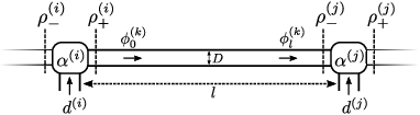
Fig. 1 illustrates the relationships between compressor constants and flux injection, flux line flow, and density variables. For notation convenience, we introduce the density variable vector .
Next, we must define a mass-flow conservation law. In this network, just as in power systems, a positive injection is defined to be a source of supply, while a negative injection represents a load. We define the load and source injection vector whose relationship satisfies
| (10) |
Matrices and codify, respectively, which lines enter and leave each node (based on the convention of the incidence matrix):
| (11) | ||||
| (12) |
where is the cross-sectional area of line . Equation (10) is a linear algebraic equation which is entirely analogous to Kirchhoff’s Current Law in an electrical network. When taking the time derivatives of Eqn (9) and (10), we have
| (13) | |||
| (14) |
Remark 2.
For notation convenience, we also define and , which are equivalent to , but un-scaled by the cross-section areas. Stated succinctly,
| (15) | ||||
| (16) |
where, again, is the signed incidence matrix.
Using the proposed notation, (7) may be written as
| (17a) | ||||
| (17b) | ||||
where is a vector of line lengths. In considering (8), we note the Hadamard product which performs element by element multiplication on a set of vectors, and Hadamard division which performs element by element division on a set of vectors. We also define function , which is a function of identically sized vectors , , and :
| (18) |
We also define a set of matrices:
| (19) | ||||
| (20) | ||||
| (21) | ||||
| (22) |
where is the vector of velocity parameters from (3), is the vector of darcy friction factors, and is the vector of pipe diameters. Thus, (8) can be written as
| (23a) | ||||
| (23b) | ||||
We may now assemble the full set of differential equations which are necessary to describe the dynamics of this network:
| (24) | ||||
| (25) | ||||
| (26) |
Next, we define the state variable vector :
and we define the RHS of the set of differential equations (24)-(26) as , such that
The full differential model is compactly stated .
Remark 3.
Before concluding this subsection, we define a NG pipeline system which has a set of specific properties.
Definition 2.
Consider a NG pipeline system whose graph has edge (line) set , , vertex (node) set , , and directed nodal incidence matrix . The graph of has a connected tree structure, meaning , and the dynamics of the network are codified by (2.3).
2.4 Degeneracy of the Flux Determined NG Simualtion Model
Now that a differential model for the flux determined model has been derived, we may investigate its shortcomings.
Theorem 1.
Consider system . The associated coefficient mass matrix is a singular matrix.
Proof.
Since the columns of are surrounded by on the top and bottom in (2.3), degenerate column rank of implies degenerate column rank of , further implying matrix singularity. Since , and , the column rank of must be degenerate. ∎
Theorem 1 implies that the implicit ODE model (2.3) is degenerate. So the solution of (2.3) should lie in the canonical subspace (canonical submanifold in nonlinear case) which is only a submanifold of the Euclidean state space [34]. This suggests that an arbitrary initial point is not necessarily consistent with the canonical subspace. Thus, the resulting trajectory may not be well-defined.
In the case where a load perturbation occurs, it would be physically meaningful to eliminate the load density and treat it as an algebraic variable which can instantaneously respond to the injection change; this observation will inform one of our proposed simulation formulations, along with the following theorem.
Definition 3.
Consider the signed incidence matrix of a tree network. The reduced incidence matrix is equal to , but with one column (any column deleted). Square matrix is known to be full rank.
Theorem 2.
Consider system . To achieve full column rank of , it is sufficient to delete a density state.
Proof.
For full column rank of to be achieved, full column rank of is necessary. To achieve full column rank of , one of its columns must be eliminated, per the proof of Theorem 1. All columns of in (2.3) are associated with a density state variable. The deletion of a column from will render a square matrix termed . Matrix is structurally equivalent to a scaled version of the system’s reduced incidence matrix. Since the reduced incidence matrix of a tree network is full rank, then so is . ∎
3 Simulation Techniques
With the observations of Theorems 1 and 2 in mind, this section introduces three alternative implicit regular ODE simulation models based on different assumptions about the nature of the sources and loads in the system.
3.1 Technique 1: Infinite Flux Reservoir
This modeling technique holds at least one pressure state in the system constant, and it has been implicitly employed in other works [26, 32, 34]. Its framework may be a poor one for investigating linepack depletion, though. Because a density state variable must be eliminated, we must delete a corresponding equation in order to ensure that the number of equations continues to match the number of state variables. The following theorem shows how non-singularity of the mass matrix can be achieved.
Theorem 3.
Consider system . The elimination of a pressure state and a flux conservation equation in (24) from will yield a square, full rank matrix .
Proof.
Once a pressure state has been eliminated, submatrix will be full rank. We define
We eliminate one row from the top subsection of (from matrices and ) and consider the rank of the submatrix , where
and the prime notation on and indicates the deletion of a row. We take the determinant of :
| (38a) | ||||
| (38b) | ||||
where since is a diagonal matrix. Since is equal to the scaled, unsigned incidence matrix of a tree network with with one node deleted, it is square and necessarily full rank. Therefore, . Because and are both full rank, it implies that matrix , which is defined by
is also full rank. ∎
Therefore, the elimination of a conservation equation from (24) and the elimination of a density state from (2.3) will yield a set of equations which can be uniquely simulated. When this happens, the density state becomes a model input, and the injection variable associated with the eliminated conservation equation is also eliminated. When the density state and conservation equation are eliminated at the same node, this node then has the interpretation of a so-called “slack" node, whose definition follows.
Definition 4.
A slack node is a node whose density (i.e. pressure) is specified and whose corresponding flux injection can take any unbounded instantaneous value to meet the specified density constraint.
The assumption behind the slack node is that it has the ability to pull from an infinite flux reservoir. This slack node is entirely analogous to the infinite bus in power system simulations, where complex power injection can take any value such that a specified complex voltage value is met.
A similar result to Theorem 3 has been suggested in [33], claiming that the DAE system is index-1 if only one supply (slack) node exists in the network. This statement is equivalent to the regularity condition of our implicit ODE model (2.3). However, in [33], compressors are not modeled; while in our ODE model (2.3) general compressors are explicitly considered.
Simulation Model Statement
To implement this simulation technique, we assume without loss of generality (WLOG) that the first node in will be treated as a slack node. We split system into the to-be eliminated conservation equation and the remaining equations :
| (42) |
We also split state variable vector into the to-be eliminated density variable and the remaining variables :
| (43) |
We parse the system according to
| (44) |
and we eliminate the top equation in (44). Finally, we parse the second equation, such that
| (45) |
The final simulation model is given by
| (46) | ||||
| (47) |
where is specified by the user. If constant pressure is assumed, and the formulation simplifies. The primary drawback of this simulation technique is that source fluxes are treated as unconstrained injections. Thus, linepack depletion cannot be explored properly in contingency situations, since the system has an infinite flux reservoir at its disposal.
3.2 Technique 2: Finite Flux Reservoir with Upper Bound Modeled via Sigmoid Function
As a realistic modification to the infinite flux reservoir model, we may hypothesize the existence of a slack node with two nonideal assumptions: (i) its flux output has a finite upper limit, and (ii) its density of injection decreases in value as flux injection saturates. The first assumption turns an infinite flux reservoir into a finite one, which enables our implicit ODE model to consider system-wide flux imbalance while retaining regularity. The second assumption stems from a more realistic consideration of satisfying the operating curves of centrifugal compressors which are widely used in the natural gas industry [43]. As the mass flux reaches its rated flow at the rated density (pressure) value, further increase of the mass flux requires a decline of the density to avoid the “choke” [43] or “stonewall” [44] phenomenon with potentially damaging vibrations.
To create this nonideal slack node, we introduce a fictitious state variable which parameterizes the mass flux flowing from a slack source. In particular, we consider a situation where the reservoir at a source has an output flow limit; we may codify this limit with a sigmoid function. Instead of imposing constant input , we parameterize it by the fictitious variable , such that the value of the input is flexible, but within a certain limit. Replacing the specified injection term with the injection function , the flux injection at the source can be written as
| (48) |
where is the sigmoid function given by
| (49) |
and the constant represents the maximum upper limit of flux which the source can produce; this limit is approached as .
As the flux flow saturates, according to the typical operating curve [43], we parameterize the density of the source node as a monotonically decreasing function of flux. To do so, we write
| (50) |
where is some nominal density of the node, and is a sigmoid function flipped about the y-axis:
| (51) |
The constant represents the flux value at which the density reaches half its nominal value, and the constant controls the speed at which the nodal density decreases as the flux injection approaches saturation33 3 The numerical value of can be inferred from the real operating curve or measurement data.. The sigmoid function could also be replaced with a fitted polynomial of arbitrary degree. Using the chain rule , the flux and density function time derivatives are
| (52) | ||||
| (53) |
As a clarification, the slack node density (pressure) is not a dynamic state variable, but knowledge of its derivative is still essential for simulating the network. We again assume, WLOG, that the first node in is treated as a slack node, with constrained flux state and algebraic density . We also reorder system such that the conservation law equation associated with the slack node is altered to (52) and placed at the end of the equation vector. Thus, by borrowing the formulation from (44), the updated system may be described according to
where is a row vector of zeros with a single 1 at index , i.e. the index of state variable . Since , then (3.2) may be simplified to
If slack flux is the final state variable in , then is
| (67) |
where is the column of matrix . By Theorem 3, matrix is nonsingular. The vector has its only nonzero (and negative definite) entry at the index of the slack node density state variable. When viewed as a perturbation of , for all practical purposes, will also be a nonsingular matrix. To simulate the system (3.2), must be inverted. By inspection, the inverse of is given by
where refers to the row of .
Theorem 4.
Matrix of (3.2) is nonsingular if .
Proof.
Since matrix is full rank, square matrix will clearly have full row rank as long as , since no linear combination of the above rows could create the bottom row. Assuming , of (52) is equal to 0 only when or , which only occur when . ∎
When a source flux injection is modeled by a sigmoid function, the fictitious state variable will tend to “blow up" when the upper flow limit is approached. This is problematic numerically, rather than physically, so a helpful workaround is to artificially constrain the growth of . This may be accomplished through the application of a constraint function to , where is a constant scalar that is chosen by the user. In our simulations, we let . Applying to in (52) we have,
| (70) |
Since increases much faster than , the term essentially forces to decline to nearly zero very rapidly. The matrix inversion expression of (3.2) can be updated by simply replacing .
Simulation Model Statement
To state the model compactly, we augment the state variable vector from (43) by adding : . We also augment by adding a zero to the bottom row to form augmented vector :
| (71) | ||||
| (72) |
This model may be used to investigate how a system responds when source mass flux flow limits are reached.
3.3 Technique 3: Constant Flux Sources
While Technique 1 assumed infinitely variable mass flux sources and technique 2 assumed constrained mass flux sources, technique 3 assumes constant (or specified) mass flux sources at all nodes. This is ultimately accomplished by converting a density state variable into an algebraic variable. According to Theorem 2, the deletion of a density state will render a mass matrix with full column rank. While Theorem 3 showed that we may delete a mass flux conservation equation to ensure full row rank, the following theorem shows that we may instead delete a momentum conservation equation from (26) to ensure nonsingularity of .
Theorem 5.
Consider system . The elimination of a pressure state and a flux momentum equation in (26) from will yield a square, full rank matrix .
Proof.
We borrow matrix from Theorem 3, but we alter its definition by the elimination of one row (row ) from the bottom subsection of instead of the top:
We now assume corresponding line connects nodes and . Our goal is to show that matrix (5) has full row rank. To do so, we remove two columns from (5): column and column . Each of these columns will have a single non-zero entry, at indices and respectively, so the row rank of the matrix necessarily drops by 2. By eliminating these columns, we are effectively eliminating line from the incidence matrix and our system is no longer fully connected. We now eliminate rows and . This effectively eliminates nodes and . By performing these operations, we are left with matrices which we define to be called , , and . Implicitly contained in and are two tree-structured subgraphs which have both been reduced. By defining
we employ the same tactics used in the Theorem 3 proof:
| (77a) | ||||
| (77b) | ||||
where since is a diagonal matrix. Matrix is in fact a nonsingular matrix, because it represents the block diagonal concatenation of two reduced (and scaled) tree incidence matrices which are in themselves both nonsingular. Since the determinant in (77) is nonzero, then the following is implied:
| (78) | ||||
| (79) |
because full row rank of a square matrix implies full column rank. Thus, (5) is a full rank matrix. By direct extension, matrix , which is defined by
is also full rank. ∎
We now leverage the results of Theorem 5 in order to define a simulation technique which allows for flux injections to be simultaneously specified at all nodes. To do so, we define a balancing node.
Definition 5.
A balancing node is a node whose flux injection is specified and whose nodal density is transformed from a state variable into an algebraic variable by solving a momentum balance equation.
The balancing node’s density variable thus becomes an algebraic variable whose value can be computed analytically. The decision of which node is chosen to be this balancing node is an important point which shall be considered later in this subsection. For now, we consider some balancing node which is connected to the rest of the tree through a single line44 4 Any node in the network can be selected as the balancing node, so long as the dynamics of an interconnecting line can be described via (83).. The momentum equation associated with its interconnection line is defined as
| (83) |
where we have neglected nodal indices for notational simplicity. Variables and refer to the flux flow and density at the balancing node, respectively. At this balancing node, we assume flux is exogenously specified. WLOG, we further assume constant flux such that . Thus, we may form a quadratic equation in :
| (84) |
The value of is a function of state variables , and along with state variable derivative . Assuming all of these values are known numerically, can be computed analytically via the quadratic formula. We thus write as a function of state variable vector and derivative :
| (85) |
To compute , we must know and numerically. The state variable values of , and are certain to be known (at each numerical time step). In the following theorem, we show that can be numerically computed without numerical knowledge of or its time derivative.
Theorem 6.
The numerical value of the flux derivative at the far end of the line attached to a balancing node may be computed without knowledge of the density at the balancing node or its derivative .
Proof.
Consider some system of equations given by
| (86) | ||||
| (87) |
where the prime notation indicates the deletion of one momentum equation, i.e. (83). The mass matrix associated with this system exactly corresponds to (5) which has been shown to be nonsingular. If the momentum equation associated with the balancing node’s line is the equation which was deleted, then (87) will not contain the density of the balancing node or its derivative. Therefore, all flux flow derivatives, including , may be solved for through matrix inversion of (5), without knowledge of or ∎
With the results of Theorem 6, we may assume there is some function which computes the necessary flux flow derivative value: . Thus, we may solve (84) via the quadratic formula if we first substitute in .
While the solution to (84) is necessary, we shall show that the model associated with this simulation technique additionally depends on the density derivative at the balancing node. The value of may be computed via the chain rule:
| (88a) | ||||
| (88b) | ||||
The vector will include flux flow derivatives as well as density derivatives. As proved in Theorem 6, the flux flow derivatives can be computed without or . The density derivatives are considered in the following theorem.
Theorem 7.
Once a balancing node has been selected, the density state derivatives may be uniquely computed.
Proof.
When the expression from (25) has been altered such that a density state derivative is removed, loses a column and is transformed into from (3). Because has been shown to be a nonsingular matrix, the system in (25) may be solved by specifying a single density derivative (i.e. the one that was removed) if both and are known.
Alternatively, instead of specifying a density derivative state to solve (25), a new linear equation may be introduced which specifies the relationship of the “eliminated" state with the remaining states. Since (88b) represents such a linear relationship, and since this relationship is physically independent from the processes used to model the relationships codified by (25), then a unique solution for the density derivative states may be solved for. ∎
We thus seek to use (88b) in order to add a new linearly independent row to . To do so, we restate (88b) as
where is the unknown vector, and known , are given by
| (90) | ||||
| (91) |
Thus, we may build augmented matrix by appropriately concatenating matrix and vector : . Finally,
Simulation Model Statement
In order to explicitly state the model associated with this simulation technique, we restate (44), but we reorder the system into such that the first equation is the momentum equation associated with the line attached to the balancing node:
| (94) |
where the first density variable is also associated with the balancing node. This system may be solved according to
| (95) | ||||
| (96) | ||||
| (97) |
where the first equation from (94) is used to build function , the results of Theorem 6 are used to build function , and the results of Theorem 7 and (3.3) may be used for taking the derivative of the density. In a large network, it may be numerically expedient to write (84) as . In noting that
| (98) |
the time derivative may be solved for by rearranging (98).
Selecting the Balancing Node
In a system where all flux injections are specified, it may not be obvious which node should be selected as the balancing node. The physical characteristics of this selection are important to consider, though. Since the balancing node’s density variable will transform into an algebraic variable, it will have the obligation of reacting instantaneously to any local imbalance or change in the system. For this reason, the node selected as the balancing node should generally be the node closest to the location of any system disturbance (e.g. loss of compressor, increase in load, loss of supply, leak in line). This choice, though, should be thought of as a dynamic choice, because if there is a subsequent perturbation at the source, the source should then be reassigned as the balancing node. In this way, any time the system is perturbed, the balancing node should be reassigned nearest to the location of the perturbation.
4 Test Results
In this section, we compare the previously derived simulation techniques via tests on the 20 node Belgium network; this system was reconstructed based on the model presented in [45], with some alterations. As shown in Fig. 2, this radial network has 19 lines and two active compressors ( and ). The longest line in the network is 98 km long, but all lines are finitely discretized into km sections (including the interconnection to the balancing node). In total, this discretization yields approximately 300 state variables in each simulation. Simulation code and network data are posted online for open source access55 5 github.com/SamChevalier/Natural-Gas-Simulations-TCNS. All simulations were performed using MATLAB’s ode23tb function on a Dell XPS laptop, equipped with an Intel i5 CPU @ 2.30GHz and 8 GB of RAM. Standard MATLAB ODE simulation tolerances and a time step resolution of s were employed. The computational time for each scenario is less than a minute.
4.1 Test 1: Sharp Load Increase at Node 16
In this test, the load at node 16 was doubled66 6 Increasing load by 90 increased total system load by 34%. in value over the course of 1000 seconds. This was accomplished by setting from (24) to from time to , as shown by in Fig. 3. This smooth load growth prevented the excitation of any high frequency transients, which the given models aren’t suitable for capturing. The system was further simulated for another 60 hours (or until bifurcation) with all three alternative modeling techniques. The following subsections describe the results of each simulation in more detail.

4.1.1 Technique 1: Infinite Flux Reservoir
In this trial, source node 8 was chosen as the constant density slack node. The density response for all system nodes (real and virtual) is shown in panel of Fig. 4 across the full 60 hours of simulation. As can be seen, after approximately 50 hours, the system converged to a new steady state operating equilibrium. The slack node was able to fully compensate for the load increase, and the flux imbalance in the system was ultimately driven to 0. The density at node 8 (the slack node) remained constant despite a precipitous fall in pressure at other nodes in the network. The pressure at node 5, which is also a source node, dropped considerably, because this source was modeled as a constant flux injector. Due to the limitless flux injection at the slack node, system linepack was never be fully depleted with this simulation model.
4.1.2 Technique 2: Finite Flux Reservoir with Upper Bound Modeled via Sigmoid Function
In this trial, source node 8 was converted from a constant density node to a node whose flux injection was constrained by (48) and whose density of injection was governed via (50). While the mass flow consumed by the load increased by 90 , was chosen such that the source could only provide an additional 60 of mass flow, inducing a sustained mass flow imbalance at -30 . Additionally, was selected. The densities for all system nodes (real and virtual) is shown in panel of Fig. 4 across the full 60 hours of simulation.
At hour 52, the linepack of a pipeline in the system was completely depleted since the gas density (pressure) at node 16 reached zero. It was caused by the constant imbalance of the mass flow rate in the system due to the overloading at node 16 beyond the injection capability of source node 8. As the flux at node 8 saturated, the linepack in the system began to deplete, and the system could no longer support the loads. When approaching node 8’s maximum injection capability, the designated density (pressure) at node 8 could not be sustained anymore. Thus, node 8 experienced a continuous density drop as well, according to our model, which further contributed to the density drop at other nodes. The whole process is in significant contrast with the Infinite Flux Reservoir model results, shown in panel , where the flux was finally re-balanced and the system stabilized to a new equilibrium point. When simulated using this model, the survival time of the system is clearly finite. This comparison validates that our proposed Finite Flux Reservoir model can capture the slow dynamics of the linepack depletion for severe contingency situations, and it can provide an estimation of the system survival time when system sources saturate.
4.1.3 Technique 3: Constant Flux Source
This model is more restrictive than the previous two, since all the source node flux inputs are rigid without any flexibility. Thus, we expected that the system could survive for an even shorter period of time. In this trial, source node 8 was selected as the balancing node77 7 This selection was made for comparison purposes. As previously noted, node 16 is actually the most suitable choice for balancing node, since this is the location of the disturbance. Its density state was thus converted into an algebraic variable and its flux injection was held fixed. The density response for all system nodes (real and virtual) is shown in panel of Fig. 4 across the full 60 hours of simulation. The linepack of the system was completely depleted since the density of node 16 reached zero after only 19 hours, though. As can be seen, the pressure in the system collapse much faster than in the previous simulation. Nodal densities drop dramatically due to the severe flux imbalance in the network.
4.2 Test 2: Partial Loss of Compressor at Node 17 during Load Increase Period
In this test, we considered a contingency where a compressor was partially compromised during a load increasing period. We restricted the load increase such that it was within the source node injection capability of the second technique in order to avoid linepack depletion. We were interested in whether the system could survive in the post-fault period, and if it could survive, how the compressor loss affected the new steady state convergence.
Specifically, the compressor at node 17 was intentionally compromised. Its original density amplification value of (i.e. ) was decreased by over the course of 2 hours using a smooth sigmoid function. Meanwhile, the loads at nodes 19 and 20 were doubled over this time period, and the load at node 18 was increased from 0 to 10 . These load changes were not beyond the maximum injection capability at source node 8 for the second technique. We further imposed that all loads had a minimum gas density (pressure) requirement of . The system was simulated for fifty hours with the three alternative techniques; the density responses for all three simulations are shown in Fig. 5.
Panel in Fig. 5 corresponds to the infinite flux reservoir model simulation. The results show that the system converged to a stable equilibrium, with the lowest density in the system being , which was greater than . Therefore, the infinite flux reservoir model predicted that the system will survive the compressor fault during the load increasing period with a workable density condition.
Panel corresponds to the bounded finite flux reservoir response. The system also converged to a stable equilibrium, but the lowest density was , which is less than . Thus, the finite flux reservoir model predicted that the system would survive the compressor fault, but some nodal densities were not workable.
Finally, panel corresponds to the constant flux source simulation. Since all the source flux was fixed in this model, the overloading condition eventually drove the system to collapse. The partial loss of the compressor, though, accelerated this process for around 26 hours.
These results can be contrasted to a situation where the loads at nodes 18-20 increase in the same manner, but the compressor at node 17 is not compromised. Density responses are seen in Fig. 6. The minimum density steady state responses of the system in panels () and () are both higher than their counterparts in Fig. 5, and both are well above . In panel (), the system does still collapse due to the flux imbalance, but the system’s survival time is increased by approximately 8 hours due to the properly functioning compressor.
These tests demonstrate that our proposed techniques can be used to simulate various contingencies under different assumptions, and are capable of predicting the system survival time under the long term mass flux imbalance condition, which is not fully captured by the commonly used model.
5 Conclusion
In this paper, three alternative implicit ODE models for studying dynamic linepack depletion in NGPNs are derived and discussed. The conventional model is shown to be degenerate under specified mass flux inputs for every node. Thus, it is not capable of characterizing linepack depletion in the case of a system-wide mass flux imbalance. The other two proposed implicit ODE models are shown to be regular (non-degenerate) under specified mass flux inputs. They are novel and present new opportunities for characterizing the survival time of NGPNs in the context of extreme contingencies.
Using the proposed methods, we simulated and analyzed two specific potential contingencies: a sudden load increase, which could be caused by the emergency dispatch of gas-fired power plants or an unanticipated large scale leakage; and the partial loss of a compressor (during a load increase period), which could be caused by the malfunctioning of a compressor station or loss of power. In terms of evaluating linepack depletion and system survival time, the simulation results validated the anticipations of the proposed models: in both simulation experiments, the system had infinite survival time when a slack node was present in the system, but finite survival time when the slack node was fully converted to a constant flux source. Also as anticipated, the survival time for the constant flux system was shorter than the survival time for the system with the finite flux reservoir. Other contingencies, such as a line leak, system bifurcation, or sudden loss of a source, will be characterized in future publications. Additionally, this framework will be useful in characterizing the interdependency of different networks and the propagation of failures between electrical power systems and NGPNs.
Acknowledgements
The authors gratefully acknowledge support by the NSF grant CNS-1735463. We also thank Prof. Paul Hines at University of Vermont, Prof. Seth Blumsack at Penn State University, Prof. Eytan Modiano at MIT, and Dr. Anatoly Zlotnik at Los Alamos National Lab for helpful discussions and useful feedback.
References
- [1] B. Tyra, Electric power monthly with data for june 2019, Tech. rep., Energy Information Administration (2019).
- [2] M. Johnson, Electric power monthly with data for october 2001, Tech. rep., Energy Information Administration (2002).
- [3] V. Ekstrom, Grid reliability and the role of natural gas, Energy Futures (May 2014).
- [4] J. A. Oliver, M. J. Samotyj, Electrification of natural gas pipeline-a great opportunity for two capital intensive industries, IEEE Transactions on Energy Conversion 14 (4) (1999) 1502–1506.
- [5] M. Chertkov, M. W. Fisher, S. Backhaus, R. Bent, S. Misra, Pressure fluctuations in natural gas networks caused by gas-electric coupling, 2015 48th Hawaii International Conference on System Sciences (2015) 2738–2747.
- [6] Y. Ruan, Q. Liu, W. Zhou, B. Batty, W. Gao, J. Ren, T. Watanabe, A procedure to design the mainline system in natural gas networks, Applied Mathematical Modelling 33 (7) (2009) 3040–3051.
- [7] C. Unsihuay-Vila, J. W. Marangon-Lima, A. Z. De Souza, I. J. Perez-Arriaga, P. P. Balestrassi, A model to long-term, multiarea, multistage, and integrated expansion planning of electricity and natural gas systems, IEEE Transactions on Power Systems 25 (2) (2010) 1154–1168.
- [8] B. Zhao, A. J. Conejo, R. Sioshansi, Coordinated expansion planning of natural gas and electric power systems, IEEE Transactions on Power Systems 33 (3) (2017) 3064–3075.
- [9] S. Misra, M. W. Fisher, S. Backhaus, R. Bent, M. Chertkov, F. Pan, Optimal compression in natural gas networks: A geometric programming approach, IEEE transactions on control of network systems 2 (1) (2014) 47–56.
- [10] S. D. Manshadi, M. E. Khodayar, A tight convex relaxation for the natural gas operation problem, IEEE Transactions on Smart Grid 9 (5) (2018) 5467–5469.
- [11] T. H. Tran, S. French, R. Ashman, E. Kent, Impact of compressor failures on gas transmission network capability, Applied Mathematical Modelling 55 (2018) 741–757.
- [12] C. Liu, C. Lee, M. Shahidehpour, Look ahead robust scheduling of wind-thermal system with considering natural gas congestion, IEEE Transactions on Power Systems 30 (1) (2014) 544–545.
- [13] M. Gil, P. Dueñas, J. Reneses, Electricity and natural gas interdependency: comparison of two methodologies for coupling large market models within the european regulatory framework, IEEE Transactions on Power Systems 31 (1) (2015) 361–369.
- [14] C. He, C. Dai, L. Wu, T. Liu, Robust network hardening strategy for enhancing resilience of integrated electricity and natural gas distribution systems against natural disasters, IEEE Transactions on Power Systems 33 (5) (2018) 5787–5798.
- [15] P. Kundur, et al., Power system stability and control, Vol. 7, McGraw-Hill New York, 1994.
- [16]
P. Sauer, M. Pai, Power
System Dynamics and Stability, Stipes Publishing L.L.C., 2006.
URL https://books.google.com/books?id=yWi9PAAACAAJ - [17]
J. Glover, M. Sarma, T. Overbye,
Power Systems Analysis
and Design, Cengage Learning, 2007.
URL https://books.google.com/books?id=MAFV_vekue0C - [18] J. Van Deen, S. Reintsema, Modelling of high-pressure gas transmission lines, Applied Mathematical Modelling 7 (4) (1983) 268–273.
- [19] A. J. Osiadacz, Simulation of transient gas flows in networks, 1984.
- [20] A. Thorley, C. Tiley, Unsteady and transient flow of compressible fluids in pipelines—a review of theoretical and some experimental studies, International journal of heat and fluid flow 8 (1) (1987) 3–15.
- [21] A. J. Osiadacz, M. Yedroudj, A comparison of a finite element method and a finite difference method for transient simulation of a gas pipeline, Applied mathematical modelling 13 (2) (1989) 79–85.
- [22] M. Abbaspour, K. S. Chapman, L. A. Glasgow, Transient modeling of non-isothermal, dispersed two-phase flow in natural gas pipelines, Applied Mathematical Modelling 34 (2) (2010) 495–507.
- [23] A. López-Benito, F. J. E. Tenreiro, L. C. Gutiérrez-Pérez, Steady-state non-isothermal flow model for natural gas transmission in pipes, Applied Mathematical Modelling 40 (23-24) (2016) 10020–10037.
- [24] M. Chaczykowski, Transient flow in natural gas pipeline–the effect of pipeline thermal model, Applied Mathematical Modelling 34 (4) (2010) 1051–1067.
- [25] A. Herrán-González, J. De La Cruz, B. De Andrés-Toro, J. Risco-Martín, Modeling and simulation of a gas distribution pipeline network, Applied Mathematical Modelling 33 (3) (2009) 1584–1600.
- [26] T. Mak, P. Van Hentenryck, A. Zlotnik, R. Bent, Dynamic compressor optimization in natural gas pipeline systems, INFORMS Journal on Computing 31 (01 2019). doi:10.1287/ijoc.2018.0821.
- [27] F. Uilhoorn, State-space estimation with a bayesian filter in a coupled pde system for transient gas flows, Applied Mathematical Modelling 39 (07 2014). doi:10.1016/j.apm.2014.06.021.
- [28] K. Wen, Z. Xia, W. Yu, J. Gong, A new lumped parameter model for natural gas pipelines in state space, Energies 11 (2018) 1971. doi:10.3390/en11081971.
- [29]
V. Gyrya, A. Zlotnik,
An
explicit staggered-grid method for numerical simulation of large-scale
natural gas pipeline networks, Applied Mathematical Modelling 65 (2019) 34
– 51.
doi:https://doi.org/10.1016/j.apm.2018.07.051.
URL http://www.sciencedirect.com/science/article/pii/S0307904X1830369X - [30] Y. Zhou, C. Gu, H. Wu, Y. Song, An equivalent model of gas networks for dynamic analysis of gas-electricity systems, IEEE Transactions on Power Systems 32 (6) (2017) 4255–4264. doi:10.1109/TPWRS.2017.2661762.
- [31]
M. Behbahani-Nejad, Y. Shekari,
Reduced order modeling of natural
gas transient flow in pipelines, International Journal of Mechanical and
Mechatronics Engineering 2 (7) (2008) 868 – 872.
URL http://waset.org/Publications?p=19 - [32]
A. Zlotnik, S. Dyachenko, S. Backhaus, M. Chertkov,
Model reduction and optimization
of natural gas pipeline dynamics, Vol. Volume 3 of Dynamic Systems and
Control Conference, 2016.
arXiv:https://asmedigitalcollection.asme.org/DSCC/proceedings-pdf/DSCC2015/57267/V003T39A002/4445521/v003t39a002-dscc2015-9683.pdf,
doi:10.1115/DSCC2015-9683.
URL https://doi.org/10.1115/DSCC2015-9683 - [33] S. Grundel, L. Jansen, N. Hornung, T. Clees, C. Tischendorf, P. Benner, Model order reduction of differential algebraic equations arising from the simulation of gas transport networks, in: S. Schöps, A. Bartel, M. Günther, E. J. W. ter Maten, P. C. Müller (Eds.), Progress in Differential-Algebraic Equations, Springer Berlin Heidelberg, Berlin, Heidelberg, 2014, pp. 183–205.
- [34] R. Lamour, R. März, C. Tischendorf, Projector based analysis of linear differential algebraic equations, Tech. rep., Technical Report 11-20, Humboldt-University, Department of Mathematics (2011).
- [35] R. Lamour, R. März, C. Tischendorf, Projector based treatment of linear constant coefficient daes, Preprint, Institute of Mathematics, Humboldt University of Berlin, Germany (2011) 11–15.
- [36] S. L. Campbell, A general form for solvable linear time varying singular systems of differential equations, SIAM journal on Mathematical Analysis 18 (4) (1987) 1101–1115.
- [37] Y. Qiu, S. Grundel, M. Stoll, P. Benner, Efficient numerical methods for gas network modeling and simulation (2018). arXiv:1807.07142.
- [38] J. C. Strikwerda, Finite difference schemes and partial differential equations, SIAM, 2004.
- [39]
M. Chaczykowski, P. Zarodkiewicz,
Simulation
of natural gas quality distribution for pipeline systems, Energy 134 (2017)
681 – 698.
doi:https://doi.org/10.1016/j.energy.2017.06.020.
URL http://www.sciencedirect.com/science/article/pii/S0360544217310125 - [40] P. Secchi, Linear symmetric hyperbolic systems with characteristic boundary, Mathematical methods in the applied sciences 18 (11) (1995) 855–870.
- [41] P. Secchi, Well-posedness of characteristic symmetric hyperbolic systems, Archive for rational mechanics and analysis 134 (2) (1996) 155–197.
- [42] J.-F. Coulombel, Well-posedness of hyperbolic initial boundary value problems, Journal de mathématiques pures et appliquées 84 (6) (2005) 786–818.
- [43] M. P. Boyce, et al., Principles of operation and performance estimation of centrifugal compressors, in: Proceedings of the 22nd Turbomachinery Symposium, Texas A&M University. Turbomachinery Laboratories, 1993.
- [44] F. T. Davis, The simulation of large industrial centrifugal compressors, Louisiana State University, 1972.
- [45]
D. De Wolf, Y. Smeers,
The
gas transmission problem solved by an extension of the simplex algorithm,
Management Science 46 (11) (2000) 1454–1465.
arXiv:https://pubsonline.informs.org/doi/pdf/10.1287/mnsc.46.11.1454.12087,
doi:10.1287/mnsc.46.11.1454.12087.
URL https://pubsonline.informs.org/doi/abs/10.1287/mnsc.46.11.1454.12087