Asymptotic regime analysis of NOMA uplink networks under QoS delay Constraints

ETIS, Information Processing and Systems Teams, is a joint research unit at CNRS (UMR 8051), ENSEA Cergy and the University of Cergy-Pontoise. ETIS is attached mainly to the Institute of Computer Science and their Interactions (INS2I). ETIS is located on the premises of ENSEA and UCP (St-Martin 1). The laboratory hosts faculty members, researchers and administrative and technical staff from these three institutions. Researchers in the laboratory report to CNRS section 7 ”Information Science: Signals, Images, Languages, Automation, Robotics, Interactions, Integrated Hardware-Software Systems”.
ETIS has over a hundred members and is structured into four research teams:

• •

  Multimedia Indexing and Data Integration (MIDI)
  The work of the MIDI team focuses on indexing, searching and searching large amounts of data, ranging from relational databases, to heterogeneous Web data (XML, RDF, information flow) and multimedia data (images, videos, 3D objects).
  The activity of the team is organized around two axes: masses of data and multimedia research systems

• •

  Information, Communications, Imaging (ICI)
  The research activities of the ICI team revolve around four axes: error correcting coding, information theory, resource allocation and imagery.

• •

  CELL, Formerly Architectures, Systems, Technologies for Embedded Reconfigurable Units (ASTRE)
  The theme of the Cell team focuses on heterogeneous systems-on-a-chip reconfigurability methods, with the originality to explore their adaptability at different levels, circuit, system and software, for many embedded applications (video, telecommunication, radiology, embedded systems for health).

• •

  Neurocybernetic
  The goal of the neuro team is to model the neural mechanisms and important brain structures of infant development to make autonomous robots that can perceive the outside world, learn for themselves and interact with it.

Non orthogonal multiple access (NOMA) schemes have attracted a lot of attention recently, allowing multiple users to be served simultaneously with enhanced spectral efficiency; it is known that the boundary of achievable rate pairs using NOMA is outside the capacity region achievable with orthogonal multiple access techniques [11] or other approaches to increase spectral efficiency [12, 10, 13]. Superior achievable rates are attainable though the use of superposition coding at the transmitter and of successive interference cancellation (SIC) at the receiver [24], [17], [14], while it is shown in [22] that NOMA is also advantageous with respect to physical layer security [6, 5, 7, 4]. The SIC receiver decodes multi-user signals with descending received signal power and subtracts the decoded signal(s) from the received multi-user signal, so as to improve the signal-to-interference ratio. The process is repeated until the signal of interest is decoded. In uplink NOMA networks, the strongest user’s signal is decoded first (as opposed to downlink NOMA networks in which the inverse order is applied).

Besides, in a number of emerging applications, quality of service (QoS) delay constraints become increasingly important, e.g., ultra reliable low latency (URLLC) systems. Furthermore, in future wireless networks, users are expected to necessitate flexible delay guarantees for achieving different service requirements. Henceforth, in order to satisfy diverse delay requirements, a simple and flexible delay QoS model is imperative to be applied and investigated. In this respect, the effective capacity (EC) theory can be employed [23],[20] [18], [19], with EC denoting the maximum constant arrival rate which can be served by a given service process, while guaranteeing the required statistical delay provisioning.

Applying the EC theory in a NOMA setting with multiple users, the $m$-th user’s EC over a block-fading channel, is defined as:

where $T_{f}$ is the symbol period, $B$ the block bandwidth and $\mathbb{E}\left[\cdot\right]$ denotes expectation over the channel gains.

The rest of the report is organized as follows: In Section 3 we present multiple access techniques, in Section 4 the theory of effective capacity (EC), in Section 5 the application of TEC in the case of two-user network uplink OMA and NOMA, in Section 6 we introduce user-pairing and multiple NOMA pairs and in Section 7 we present our simulation results.

Multiple Access techniques are classified into two major families: orthogonal and non-orthogonal.

In the uplink, the BS will first decode the symbol of the strongest user treating the transmission of the weaker one as interference. After decoding it suppresses it from $Z$ and will decode the signal of the next strongest user. Following the SIC principle, and denoting by $\rho=\frac{1}{\sigma^{2}}$ the transmit SNR, the achievable rates, in b/s/Hz, for the $m^{th}$ user is expressed as [8]:

Replacing (4) into (), we obtain the following expression for the EC of the $m^{th}$ user:

where $\beta_{m}=-\frac{\theta_{m}T_{f}B}{\ln{2}}$ is the normalized (negative) QoS exponent for $m=\{1,2,..,M\}$.

To account for the ordering of the channel gains we make use of the theory of order statistics in the following analysis [21]. Assume a network of $M$ users with $|h_{1}|^{2}<|h_{2}|^{2}<...<|h_{M}|^{2}$, $x_{m}=|h_{m}|^{2},m=1,2,...M$ to denote independent and identically distributed (i.i.d.) random variables with underlying probability density function (pdf) $f(x_{m})$. Ranking these random variables using order statistics we obtain:

where $f_{\gamma_{m:M}}$ denotes the pdf of the $m$-th ordered random variable in a population of $M$ (in the two-user case $M=2$), $\psi_{m}=\frac{1}{B(m,M-m+1)}$, and, $B(a,b)$ is the beta function $B(a,b)$=$\frac{\Gamma(a)\Gamma(b)}{\Gamma(a+b)})$, with $\Gamma(a)=a!$. Finally, $F(x)$ denotes the cumulative density function (cdf) of the the random variable $x_{m}$, $m=\{1,2\}$.

Assuming a Rayleigh wireless environment, the NOMA gains of the channel, denoted by $x_{m}$, are exponentially distributed with respective pdf and cdf respectively [15]

The general expression of the EC of the $m^{th}$ user in a $M$ users uplink NOMA scenario can be expressed as:

where $f_{\gamma_{1:2:3:...M}}(x_{1},x_{2},...,x_{m})$ is the joint distribution of $x_{i}$, $i=1,2,..,m$.

After analyzing the two-user NOMA network, we investigate the total achievable link-layer rate for multiple NOMA pairs in the uplink scenario. For $M$ users, we get $\frac{M}{2}$ groups with these following index $i=1,2,..,\frac{M}{2}$, where each group contains 2 users. Inside each group, NOMA is implemented, and for inter-group TDMA is assumed to be applied.

The achievable data rate of the two users $1^{st}$ and $2^{nd}$ of the $i^{th}$group, where $|h_{1,i}|^{2}\leq|h_{2,i}|^{2}$ can be formulated as follows:

On the other hand, if users 1 and 2 each have their message transmitted using TDMA, the achievable data rate is as follows (here we make use of the fact that $P=P_{1}+P_{2}=1$ and we omit the total power $P$):

$\frac{1}{M}$ means that each user has only one time slot to transmit. And $\frac{2}{M}$ is a resource available for the two users inside a NOMA group.

By replacing (20) and (21) in (1) we get respectively the following ECs of the $1^{st}$ and $2^{th}$ user of the $i^{th}$ group:

On the other hand, replacing (22) in (1) we get the expressions for both users while using TDMA scheme:

Here, we analyze the total EC of multiple NOMA pairs, denoted $W_{N}$, in comparison with the total EC for the $M$ OMA users, $W_{O}$,

and

As in [24], to investigate the region of $\rho$ in which NOMA offers higher total link-layer rates EC compared to OMA, the following Lemma is provided.
Lemma 6: Considering the difference between the total EC of multiple NOMA pairs and the OMA, we prove that: a) When $\rho\rightarrow 0$, $W_{N}-W_{O}$$\rightarrow 0$, and
$\lim\limits_{\rho\rightarrow 0}\frac{\partial(W_{N}-W_{O})}{\partial\rho}=\sum_{i=1}^{\frac{M}{2}}\Big(\frac{2P_{1,i}-1}{M\ln 2}(\mathbb{E}[|h_{1,i}|^{2}]-\mathbb{E}[|h_{2,i}|^{2})\Big)\geq 0$
b) When $\rho\rightarrow\infty$, $W_{N}-W_{O}$$\rightarrow Q$, given in (29), and $\lim\limits_{\rho\rightarrow\infty}\frac{\partial(W_{N}-W_{O})}{\partial\rho}=0$

where

The proof is provided in Appendix H.

From Lemma 6, we can conclude that $W_{N}-W_{O}$ starts initially at 0, it fist increases at small values of transmit SNR $\rho$, and finally approaches a constant Q given in (29), at high values of the transmit SNR. That means multiple NOMA pairs outperforms OMA for low transmit SNRs. And this performance gain of NOMA over OMA becomes stable when the transmit SNR is extremely high.

In this section the proposed Lemmas in the previous sections will be validated through Monte Carlo simulations. We considered a two user uplink NOMA system, with the following setting: transmission power of users, $P_{1}$=0.2, $P_{2}$=0.8 (i.e power coefficients $\alpha_{1}$=0.2, $\alpha_{8}$=0.8, and the total power $P$=1) and we set the normalized delay exponent equal to $\beta_{1}$=$\beta_{2}$=-1 for both users.

To confirm the accuracy of the proposed closed-form expressions for EC in NOMA scheme for both users, we used Monte Carlo simulations. Figure 5 shows the curves of the both users effective capacities, $EC^{1}$ and $EC^{2}$, using the closed-form expressions and using the Monte Carlo. So the accuracy of these closed-form can be confirmed, except in the very low SNR region (discrepancy).

Figure 6 includes the plots for the EC of the uplink two-user NOMA and OMA system versus the transmit SNR. We note that for the weak user, OMA is better than NOMA for low transmit SNRs, and NOMA is better than OMA at high transmit SNRs. In the contrary, for the strong user, NOMA is better than OMA at small values of SNR, and OMA is better at high values of the transmit SNR. We notice also that the EC of the strong is limited, it reaches a plateau at high SNR. This provides numerical validation of Lemma 1.
Figures 7 and 8, show respectively the EC of user 1 and user 2, versus the transmit SNR, for several value of delay. when the delay become more stringent, i.e $\beta$ decreasing ( delay QoS increase), the individual link-layer rates in NOMA decreases, for the both users.

In Figure 9, the ECs of the strong and weak users are depicted as functions of the delay exponent, for NOMA and OMA scenarios. We note that EC in uplink NOMA and that in OMA are identical for both user.

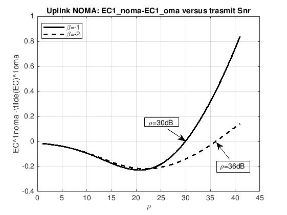
Figure 11 shows the difference of the EC in NOMA and the EC in OMA of the weak user. This curve starts initially at zero, then decreases to a certain minimum and starts increasing at high values of the transmit SNR. This confirms the Lemma 2. When the delay is equal to -1, we see that between 0 and 30 dB, the curves are negative, that means OMA outperform NOMA in this range. But After 30dB, the curves is positive, which means that NOMA offers better link-layer rate. However, that range O-30dB (where OMA outperforms NOMA) is not a general thing, we notice that by changing the transmission powers of users that range also changes. By increasing the transmission power of the weak user and reducing the transmission power of the strong user, we notice that the range is reduced. That range expands when we do the inverse. Also, when the delay becomes a little bit more stringent, $\beta_{1}$=$\beta_{2}$=-2, the zero crossing moves from 30 to 36 dB.

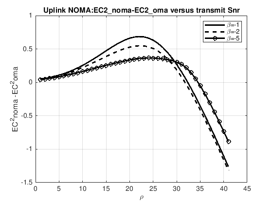
Figure 12 shows the difference of the EC in NOMA and the EC in OMA of the strong user. This curve starts initially at zero, then increases to a certain maximum and starts decreasing to infinity at high values of the transmit SNR. This confirms Lemma 3. We note that the maximum of these curves decreases when the delay becomes more stringent.

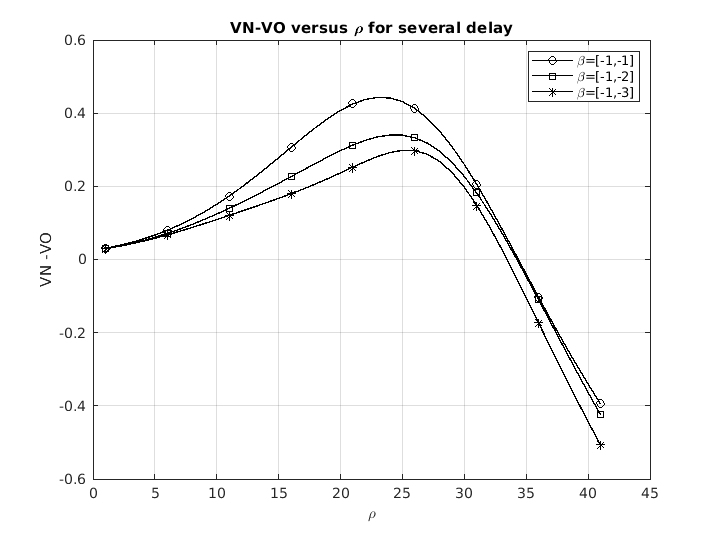
To investigate the impact of $\rho$ on the performance of the total link-layer rate for the two-user system, Figure 13 includes the plots for $V_{N}$ in NOMA and $V_{O}$ in OMA, versus the transmit SNR, for various delay. This figure shows that for both NOMA and OMA, the total EC for the two users, starts at the initial value of 0 and starts increasing with the transmit SNR. This confirms the Lemma 4.a and Lemma 4.d. This figure shows that when $\rho$ is very small, the total link-layer rate for the two user in NOMA, $V_{N}$, has a faster increasing slope than $V_{O}$ in OMA. On the contrary, with the increase of the transmit SNR, $V_{O}$ becomes gradually higher than $V_{N}$. Further, at very high values of the SNR, the gap of the total EC between NOMA and OMA becomes unstable. And when the delay becomes more stringent, the total EC of both NOMA and OMA decreases.

Figures 14 and 15 depict the plots of EC versus $\rho$, for several normalized delay values. In figure 14, the delay of the strong user is fixed. And we see that when delay of the strong user is fixed, the highest delay QoS (i.e smallest normalized delay $\beta$) of the weak user gives us the highest level of the $V_{N}-V_{O}$. On the other hand, when the delay is fixed, Figure 15 shows that, the smallest delay Qos (i.e highest normalized delay $\beta$) value of the strong user gives us the highest level of the $V_{N}-V_{O}$.

The curve of $V_{N}-V_{O}$ starts at zero, increases to a maximum, and returns to zero. The transition to zero is at $\rho$ = 31, and $\rho$ =36 respectively for the figures 14 and 15. That means from 0 to 31dB (36dB in the Figure 15), the total link-layer rate of NOMA is higher than the OMA one. And After this transition to zero, the total link-layer rate OMA outperforms the NOMA one.

Then we focus on the comparison of multiple NOMA pairs and OMA in term of the total link-layer rate, i.e $W_{N}$-$W_{O}$. The figure 16 depicts the curve of the total link-layer of NOMA pairs, $W_{N}$, and the total link-layer of the OMA, versus the transmit SNR. The multiple NOMA pairs scheme outperforms the OMA. The performance gain of NOMA multiple users pairs over OMA start at zero, increases at small values of SNR, and becomes steady at high transmit SNRs.

Figure 17 shows the curves $W_{N}-W_{O}$ versus the transmit SNR, for various setting of the user-pairing. It starts at zero at small value of $\rho$, increases until it reaches a maximum, at high values of $\rho$. This Confirmes Lemma 6. Specifically, we set the total number of users M=4, the power coefficients allocated to both users in a NOMA pair are given as P1=0,2 and P2=0.8 in all the groups and the normalized delay of all users are assumed to be equal $\beta_{1,i}$=$\beta_{2,i}$=-1, ($i=1,2,..,\frac{M}{2}$).

The concept of the effective capacity enabled us to study the achievable data link layer rates when QoS delay guarantees are in place in the form of delay exponents. In this report, we have investigated the effective capacity of the uplink of a two-user NOMA network, assuming a block Rayleigh fading channel. We derived novel closed-form expressions for the two users in a two user-uplink NOMA network. We validated the proposed mathematical formulas with Monte Carlo simulations. We provided a comparison between a uplink NOMA two-user network and OMA uplink two-user network. We also analysed the impact of user-pairing on the total link, we showed that when pairing is used the total link layer rate is higher than the OMA one, and we found a best power allocation policy in the case four users, i.e., we found the set of pairs which gives the highest total link layer rate. We showed that the ECs of both users decrease as the delay constraints become stringer. On the other hand, at high transmit SNRs, the EC of the weak user can surpass the EC of the strong user, as the latter is limited due to interference.

In the uplink NOMA, the strong user decodes the message of all weaker users, before its own message. This is a problem from a security point of view. An eavesdropper can exploit this flaw to intercept communications. The next challenge is to find the maximum achievable link layer that can be achieved while guaranteeing secure communications. For that, another metric that has recently been defined can be used, the effective secrecy capacity (ESC) [22], [16],[9]. A performance analysis using that metric could be subject to future work, in the uplink NOMA scenario.

Appendix A

From (16) we have:

Set $t=\rho P_{1}x_{1}$ i.e., $x_{1}$=$\frac{t}{\rho P_{1}}$ and since $x_{1}$:0$\rightarrow\infty$, $t$:0$\rightarrow\infty$, $dx_{1}$=$\frac{1}{\rho P_{1}}dt$.

Replacing these in (25):

setting, $a=1,(b-a-1)=\beta_{1}$, i.e., $b=\beta_{2}+2$. $z=\frac{2}{P_{1}\rho}$ and having the $U\left(.,.,.\right)$ the confluent hypergeometric function U(a,b,z) defined as follow:
$U(a,b,z)=\frac{1}{\Gamma(a)}\int_{0}^{\infty}e^{-zt}t^{a-1}(1+t)^{b-a-1}dt$
We have:

Finally we have the closed-form expression of the User 1:

For the second user, by replacing from (17) have:

Setting $z=\frac{1+\rho P_{1}x_{1}}{\rho P_{2}}+x_{2}$, we have: $x_{2}=z-\frac{1+\rho P_{1}x_{1}}{\rho P_{2}}$ and $dx_{2}=dz$, so that when $x_{2}\rightarrow x_{1}$, $z\rightarrow\frac{1+\rho P_{1}x_{1}}{\rho P_{2}}+x_{1}=\frac{1+\rho x_{1}}{\rho P_{2}}$ and when $x_{2}\rightarrow\infty$, $z\rightarrow\infty$

we note that $\int_{a}^{\infty}\frac{e^{-x}}{x^{b}}dx=a^{-\frac{b}{2}}e^{-\frac{a}{2}}\mathbf{W}_{-\frac{b}{2},-\frac{1-b}{2}}(a)$ , where $\mathbf{W}$ is the Whittaker W function. i.e.,

References

• [1] https://www-etis.ensea.fr/.
• [2] https://www.polytechnichub.com/difference-fdma-tdma/.
• [3] Matthieu R Bloch and J Nicholas Laneman. Strong secrecy from channel resolvability. IEEE Transactions on Information Theory, 59(12):8077–8098, 2013.
• [4] A. Chorti. Masked-ofdm: A physical layer encryption for future ofdm applications. In IEEE Globecom Workshops, pages 1254–1258, 2010.
• [5] A. Chorti, C. Hollanti, J.C. Belfiore, and H.V. Poor. Physical layer security: a paradigm shift in data confidentiality. Lecture Notes in El. Eng.: Physical and data-link security techniques for future communication systems, 18(12), 2019.
• [6] A Chorti and H.V. Poor. Faster than Nyquist interference assisted secret communication for OFDM systems. In Proc. IEEE ASILOMAR, 2011.
• [7] A Chorti and H.V. Poor. Achievable secrecy rates in physical layer secure systems with a helping interferer. In Proc. Int. Conf. Computing, Networking Comms (ICNC), 2012.
• [8] Li Fan, Shi Jin, Chao-Kai Wen, and Haixia Zhang. Uplink achievable rate for massive MIMO systems with low-resolution ADC. IEEE Communications Letters, 19(12):2186–2189, 2015.
• [9] Jie Hou and Gerhard Kramer. Effective secrecy: Reliability, confusion and stealth. In 2014 IEEE International Symposium on Information Theory, pages 601–605. IEEE, 2014.
• [10] Arsenia Chorti Ioannis Kanaras and, Miguel Rodrigues, and Izzat Darwazeh. Investigation of a semidefinite programming detection for a spectrally efficient fdm system. In Proc. IEEE Int.l Sym. Personal, Indoor Mobile Radio Commun., pages 2827–2832, 2009.
• [11] SM Riazul Islam, Nurilla Avazov, Octavia A Dobre, and Kyung-Sup Kwak. Power-domain non-orthogonal multiple access (noma) in 5g systems: Potentials and challenges. IEEE Communications Surveys & Tutorials, 19(2):721–742, 2016.
• [12] I Kanaras, A Chorti, M Rodrigues, and I Darwazeh. An optimum detection for a spectrally efficient non orthogonal FDM system. In Proc. 13th Int. OFDM Workshop, Hamburg, pages 65–69. IEEE, 2008.
• [13] I Kanaras, A Chorti, M Rodrigues, and I Darwazeh. An overview of optimal and sub-optimal detection techniques for a non orthogonal spectrally efficient fdm. In academia.edu, 2009.
• [14] Rihem Nasfi and Arsenia Chorti. Performance analysis of the uplink of a two user NOMA network under QoS delay constraints. In Proc. IEEE 11th Int. Conf. Ubiquitous Future Networks (ICUFN), 2019.
• [15] Athanasios Papoulis and S Unnikrishna Pillai. Probability, random variables, and stochastic processes. Tata McGraw-Hill Education, 2002.
• [16] Deli Qiao, Mustafa Cenk Gursoy, and Senem Velipasalar. Secure communication over fading channels with statistical QoS constraints. In 2010 IEEE International Symposium on Information Theory, pages 2503–2507. IEEE, 2010.
• [17] Y. Saito, Y. Kishiyama, A. Benjebbour, T. Nakamura, A. Li, and K. Higuchi. Non-orthogonal multiple access (NOMA) for cellular future radio access. In 2013 IEEE 77th vehicular technology conference (VTC Spring), pages 1–5. IEEE, 2013.
• [18] J. Tang and X. Zhang. Cross-layer modeling for quality of service guarantees over wireless links. IEEE Transactions on Wireless Communications, 6(12):4504–4512, 2007.
• [19] Yue Tian, Xianling Wang, and Zhanwei Wang. On the performance of security-based nonorthogonal multiple access in coordinated multipoint networks. Wireless Communications and Mobile Computing, 2018, 2018.
• [20] D. Wu and R. Negi. Effective capacity: a wireless link model for support of quality of service. IEEE Transactions on wireless communications, 2(4):630–643, 2003.
• [21] Hong-Chuan Yang and Mohamed-Slim Alouini. Order statistics in wireless communications: diversity, adaptation, and scheduling in MIMO and OFDM systems. Cambridge University Press, 2011.
• [22] W Yu, A Chorti, L Musavian, and Q Ni HV Poor. Effective secrecy rate for a downlink NOMA network. IEEE Trans. on Wireless Comms, 18(12), 2019.
• [23] W. Yu, L. Musavian, and Q. Ni. Tradeoff analysis and joint optimization of link-layer energy efficiency and effective capacity toward green communications. IEEE Transactions on Wireless Communications, 15(5):3339–3353, 2016.
• [24] W. Yu, L. Musavian, and Q. Ni. Link-layer capacity of NOMA under statistical delay qos guarantees. IEEE Trans. Comms, 66(10):4907–4922, 2018.
• [25] Wenjuan Yu, Leila Musavian, and Qiang Ni. Multi-carrier link-layer energy efficiency and effective capacity tradeoff. In 2015 IEEE International Conference on Communication Workshop (ICCW), pages 2763–2768. IEEE, 2015.