An arbitrary order Mixed Virtual Element formulation for coupled multi-dimensional flow problems
Abstract
Discrete Fracture and Matrix (DFM) models describe fractured porous media as complex sets of 2D planar polygons embedded in a 3D matrix representing the surrounding porous medium. The numerical simulation of the flow in a DFM requires the discretization of partial differential equations on the three dimensional matrix, the planar fractures and the one dimensional fracture intersections, and suitable coupling conditions between entities of different dimensionality need to be added at the various interfaces to close the problem. The present work proposes an arbitrary order implementation of the Virtual Element method in mixed formulation for such multidimensional problems. Details on effective strategies for mesh generation are discussed and implementation aspects are addressed. Several numerical results in various contexts are provided, which showcase the applicability of the method to flow simulations in complex multidimensional domains.
Keywords:
Mixed VEM, DFN, Subsurface flow, Inter-dimensional coupling1 Introduction
There are many practical contexts where effective flow simulations in underground fractured media are strategic, including geothermal applications, protection of water resources, Oil&Gas enhanced production and geological waste storage. Taking advantage from an increased and easily available computational power, several problems not considered in the past have been tackled. Regardless of the application, they all share the demand for high accuracy and reliability in the results. On the other hand, due to the complexity of the typical domains of interest and to the high uncertainty of the data, effective simulations of underground phenomena are still extremely challenging, such that the research for robust and efficient numerical methods for underground flow simulations still attracts great interest from the scientific community.
In this work, the computation of the hydraulic head distribution in the subsoil is considered. The physical components of the problem are a rock matrix with an embedded network of fractures. Fractures are thin regions of the soil with different properties from the surrounding bulk material, and have one spatial dimension, the thickness, that can be orders of magnitude smaller than the domain size. For numerical simulations, the simultaneous representation of the fracture-thickness scale and of the domain-scale is unfeasible as would result in an extremely large number of unknowns, such that models are introduced to represent subsoil. Next to homogenization techniques [57], dual and multy-porosity models [25], or embedded discrete fracture matrix (EDFM) models [46, 49], Discrete Fracture and Matrix (DFM) models aim at an explicit representation of the underground fractures, which are dimensionally reduced to planar interfaces into the porous matrix. Fractures are generated randomly following probability distribution functions concerning their geometrical (position, orientation, density) and hydraulic properties. The quantity of interest is the hydraulic head distribution, which is governed by the Darcy law in the porous matrix, and by an averaged-across-thickness Darcy law in the fracture planes, plus additional coupling conditions at fracture/matrix interfaces an at the intersections between fractures, [48]. Despite the dimensional-reduction operated on the fractures, DFM models are still highly complex and multi-scale: this is a consequence of the random orientation of the fractures that usually form an intricate system of intersections, with the presence of fractures with different sizes and forming intersections that might span various orders of magnitude. In fact one planar fracture in a DFM might have an intersection of few centimeters length with one fracture and of several kilometers with another fracture, with also the smaller intersection having a relevant impact on the flow pattern. This geometrical severity, combined to the stochastic nature of simulation data, demands numerical tools robust to complex geometries and highly efficient, thus allowing to perform repeated simulations on random geometries necessary to obtain statistics on the output quantities of interest.
DFM models are widely used for underground flow simulations [4, 1, 22, 5, 19], the major complexity being the generation of a conforming mesh of the domain. The generation of a conforming mesh for the imposition of the matching conditions at the various interfaces, might in fact result in an impossible task, for the extremely high number of geometrical constraints for fracture networks of practical interest. Further the mesh generation process with conventional strategies is a global process for the whole domain, which usually requires an iterative process that might not converge. In some cases the rock matrix can be neglected, as almost impervious compared to the fractures, with the subsurface flow mostly determined by the fracture distribution. These are called Discrete Fracture Network (DFN) [34, 36, 50, 55] problems, with an only partially mitigated geometrical complexity.
Over the last decade, there has been a great development of numerical methods to tackle the problem of efficient flow simulations of realistic DFM/DFNs. An efficient algorithm for conforming discretizations have been proposed by [51]. The complexity of DFN flow simulations is reduced in [53, 52] by removing the unknowns in the interior of the fractures, reducing the dimension of the problem and rewriting it at the interfaces. The mesh conformity requirement at the interfaces in DFMs can be relaxed by using eXtended Finite Elements (XFEM) [38] as in [41, 37]. In [20, 18, 19], an optimization approach is proposed for both DFN and DFM problems which avoids any need for mesh conformity at the interfaces and instead seeks the solution as the constrained minimum of a functional representing the error in the fulfillment of interface conditions. In recent times, techniques as the Mimetic Finite Difference method (MFD) [47] have been used for flow simulations in DFMs by [3, 5], or as Hybrid High Order (HHO) methods by [24], where a partial non-conformity is allowed between the mesh of the porous medium and of the fractures. Other approaches use two or multi-point flux approximation based techniques, [58, 44, 45, 35] for DFN and DFM problems, or gradient schemes [22]. A survey on various conforming and non-conforming discretization strategies for flow simulations in networks of fractures can be found in [40].
The recently developed Virtual Element Method (VEM) [23, 8, 7] is gaining increasing interest in the field of the numerical simulation of underground phenomena as it allows to handle mesh of polygonal/polyhedral elements and is robust to badly shaped and elongated elements [15], thus allowing to easily generate conforming polygonal/polyhedral meshes in complex geometries. This method was applied, e.g., in [12, 13, 11, 39] for DFN simulations, and in DFM problems in [42] for flow computation, in [17] coupled to the Boundary Element method and in [26] coupled to finite volumes for poro-elasticity problems in DFMs.
The present work proposes an arbitrary order mixed VEM-based approach for the computation of the flow in poro-fractured media, following the DFM model proposed by [54]. A mixed formulation is a widely common choice for underground flow simulation for its mass conservation properties [48, 31, 41, 56, 59, 2, 3, 5]. The approach is an extension of the work proposed in [13] and [14], as now the VEM-based conforming approach includes the rock matrix in the problem domain, and differs from other VEM based approaches for the strategy used to obtain the computational mesh. Further, to the best of authors knowledge, this is the first arbitrary-order implementation of mixed virtual elements for flow simulations in DFM problems.
The manuscript is organized as follows: in Section 2 the formulation for the problem at hand is presented. Section 3 described the mesh generation process, whereas Section 4 is devoted to providing a description of the mixed formulation of the Virtual Element Method in the present context. Implementation is discussed in Section 5. Next, numerical results are described in Section 6, where convergence analysis of the method is proposed and problems on increasingly complex configurations are solved and analyzed. The work ends with some concluding remarks in Section 7.
2 Problem formulation
2.1 DFN problem formulation
The present section is devoted to briefly recall the formulation of the flow problem in fractured porous media with the Discrete Fracture and Matrix model, referring to [21] for a more detailed description and for well posedness results.
Let us consider a three dimensional block of porous material crossed by a network of fractures. According to the DFM model, fractures are represented as planar polygons , , which might intersect forming intersection segments , , also called traces. Further, traces can meet at intersection points , . For uniformity of notation, a subscript will be indicated also for , with the assumption that , and . We then denote by the union of all fractures, by the union of all traces, and by the union of all trace intersections. Problem domain is thus mixed dimensional, as it involves a 3D problem in , 2D problems on the fractures , 1D problems on the traces and 0D problems at trace intersections . Each domain , does not include lower dimensional domains, i.e. , such that internal boundaries are present. For , the internal boundary of domain , , is the portion of boundary that matches a sub-dimensional domain, the remaining being instead the external boundary.
For each domain , , , let us introduce the index set , containing indexes such that,if , coincides with a portion of the boundary of , i.e. . It is further set . Similarly, for , contains indexes of domains , such that , for has a non empty intersection with the boundary of .
For , we denote by and the Dirichlet and Neumann part, respectively, of the external boundary of , , , and by , the boundary of around the lower dimensional domain , , with fixed arbitrarily chosen sign for each of the two sides. For , is used to denote the unit normal vector to in , outward pointing, and, for , is the unit vector tangential to at the boundary points , outward pointing. An exemplification of the used nomenclature is proposed in Figure 2.1, for a simple DFN counting three fractures, three traces and one trace intersection.

A Darcy-type equation governs the flow problem on each geometrical dimension and suitable matching conditions couple the problems: for we have
with boundary conditions, for , ,
and coupling conditions for
In the previous equations, for , , represents a source term, the operator denotes the jump across the interface, i.e.
whereas, for , is the fracture transmissivity in and is the transmissivity in the direction normal to , with clear extension to the case . Homogeneous Neumann and Dirichlet boundary conditions are used in order to simplify the exposition. The choice of homogeneous Neumann boundary conditions for external boundaries of domains , , not touching the boundary of is widely adopted, see e.g. [48, 5, 54], other generalizations being straightforward.
Let us now move to the weak formulation of the previous problem. Let us introduce, for , , the functional spaces , and for the spaces . It is then possible to write the problem in mixed weak formulation as: for , , find , and for , find such that, for all , :
| (2.1) | |||||
| (2.2) | |||||
| (2.3) |
The used coupling equations state that the drop of pressure is proportional to , which is a sort of Darcy’s law for interdimensional flux exchange. In the limit when , and for geometrical parameters as fracture width, trace diameter that are very small compared to the other dimensions, these coupling conditions can be modeled as requiring that the pressure be continuous across fractures, traces and trace intersections; further, the third term in (2.1) vanishes. This means, for instance, that there would be no jump in pressure in a path that leaves the matrix, goes through a fracture, enters the trace network and eventually re-enters the matrix. In this case, the discrete solution should converge to a pressure field that is globally continuous across all domains.
3 Mesh generation
A key aspect of a numerical tool for the simulation of flow problems in mixed-dimensional domains with complex geometries is the generation of the computational mesh, as usually this is a non trivial and computationally expensive procedure. The meshing for standard discretization methods, as Finite Volumes or Finite Elements, is, indeed an iterative process, aiming at building good quality elements from the three dimensional down to the one dimensional domains which are perfectly matching, i.e. conforming, at the various interfaces. For non trivial geometries this process is likely to fail or to produce an extremely large number of elements, independently of the required level of accuracy, due to the need to honor the geometrical constraints.
The use of polyhedral/polygonal meshes, in conjunction with the robustness of virtual elements to badly shaped elements [16], allows instead to define an easy meshing process, which can be performed in a non iterative manner. The starting point is a general polyhedral mesh of the closure of the three dimensional domain , built independently of any lower dimensional domain contained in it, and thus not conforming to the interfaces. Let us then consider a generic element of such mesh, crossed by some two dimensional domains, possibly intersecting in it or ending in its interior. Figure 3.1 shows an example where a cubic element is crossed by two fractures, and . The element can be easily cut into sub-elements not crossing the fractures, eventually prolonging the cut, for fractures ending in the interior of the element, up to element boundary. Please observe that the geometry of the fractures is not altered in any way, as the original fracture boundaries are preserved and, when the cut is prolonged over fracture boundaries, co-planar “hanging” faces are introduced. Also “hanging” faces appear on elements neighboring cut elements. Once this process is completed, the mesh on the 2D domains is obtained simply collecting the faces of the 3D elements laying on each fracture plane as a “patchwork”, and similarly for the 1D domains. The resulting mesh is thus conforming.

4 Mixed Virtual Elements
In the following, an outline of the main definitions and features of the mixed formulation of VEM is presented. Its initial introduction is given in [23], with a follow-up work generalizing the method [8] and a related work on virtual and spaces in [9]. A thorough description of mixed VEM spaces for the Stokes, Darcy and Navier–Stokes equations is given in [33]. Despite its recent introduction, a variety of applications can be found in the scientific literature. Namely, Stokes flow in [29] and [27], the Brinkman problem [28], plane elasticity [6] and flow in networks of fractures in an impervious matrix [14].
Let us consider a domain , for and , whose mesh, comprised of arbitrary polyhedra with mesh parameter , is indicated by , and satisfies basic regularity conditions as in [23]. In the following we will drop the domain index , for simplicity of notation, as this plays no role in the discussion.
Let us then introduce a local VEM space for the velocity variable on an element , thus a polyhedron for or a polygon for , and, to this end let us denote by the space of polynomials of maximum order , in , with the additional conventional notation , for . The local VEM space on element is denoted as:
| (4.1) |
where denotes a face for or an edge for . Depending on the choice of , this space might represent an extension of BDM elements to general elements, for , , termed BDM-VEM, or an extension of Raviart-Thomas elements, for , , labeled RT-VEM. Other choices are also possible, even if not considered here [9]. The local space for the pressure variables on element , , is . We remark that BDM elements will be used only for the discretization of the 3D equations, to have the same polynomial accuracy for the pressure and the face-normal fluxes that are coupled by equation (2.2), for .
The discrete global space on , , is
resulting in a conforming space. The global space for the pressure variable is
while for the degrees of freedom of are the values at domain , . The dimension of the space is , and a basis for this space can be chosen as the monomial base :
where is the centroid of element and its diameter.
We then define the space
| (4.2) |
with dimension , and by the orthogonal complement of in so that , whose dimension is .
The DOFs of a function in , following [8] are:
| (4.3) | ||||||
A proof of unisolvence can be seen in [23, 8] for BDM- and RT-VEM respectively. The first set of DOF can be replaced by any other way to fix a polynomial of degree on a face. A listing of the dimensions of some of the polynomial spaces involved in the definition of the DOF is provided in the Supplementary Material to the present manuscript, along with a graphical exemplification of the DOFs for a convex hexagon and convex polyhedron.
For the pressure space any set of DOFs that univocally determines a polynomial of order in dimension could be adopted, as, for example, distinct point values. However, for computations, it is advantageous to take as DOFs the moments with respect to the monomial basis of order , since element geometry can be arbitrary.
Let us now introduce the projection operator as:
| (4.4) |
It can be observed that knowledge of the functions at the DOFs is enough to compute the projector. The left hand side of (4.4) is an integral between polynomials in dimension , and can be explicitly computed by a suitable quadrature rule. For the left hand side, since , we can find and such that . Thus,
| (4.5) |
The second term on the right hand side of this equation can be obtained directly from the set of DOFs of type , and, for the other term, we have that there is a polynomial such that so that applying integration by parts we obtain
| (4.6) |
Once again, the second term on the right hand side can be computed directly as an integration on the faces/edges of the 3D/2D element, by using the DOFs of type . For the first term, this can be computed once is defined, as follows:
| (4.7) |
using the set of DOFs of type and .
Let us now introduce a discrete counterpart for the bi-linear form in equation (2.1), restricted on an element , for , with , which, for reads as:
| (4.8) |
where stands for any symmetric and definite positive bilinear form that scales like on the kernel of . Specifically, there exist two positive constants and independent of the mesh and data such that
| (4.9) |
is usually taken as the standard Euclidean product of the vector of values at the DOFs scaled by the measure of and an approximation of at the barycentre or its average on the element. More precisely,
| (4.10) |
where stands for evaluating at the i-th DOF on the element, i.e. the linear operator , defined as evaluating at the -th DOF.
Finally, the global discrete bilinear form is defined as
| (4.11) |
The discrete version of the weak form of the problem specified in Eqs. (2.1)-(2.3) is then obtained replacing the continuous variables with their discrete counterparts, using the projection of the VEM shape functions for (4.8). No projection is required for terms involving the discrete pressure variable. With classical assumptions on the data, well posedness of this problem is due to continuity and coercivity of and the assumptions on as well as the satisfaction of an inf-sup condition [23, 8, 21].
5 Implementation
The details for an implementation of the three dimensional mixed formulation of the VEM method is provided. The main reference for this section is [30], from where much of the procedures provided here are inspired. Further insight for more general problems is given in [33].
5.1 Computation of the local stiffness matrix
In this section we address the computation of the local stiffness matrix on a general 2D or 3D polytope , where Virtual Element spaces are used.
In the following, it is assumed that numerical computations of integrals of known functions over 2D and 3D polytopes can be performed. The most straightforward approach is to divide a polygon into triangles, or a polyhedra into tetrahedrals and use standard Gaussian integration. Alternatives are to consider cubature [43], algebraic integration by parts or heuristic methods (like Montecarlo integration). The procedure for computing the local matrices needed to obtain the discrete linear system is explained next, with emphasis on its implementation in 3D. First we consider a basis of denoted by , where the basis functions are chosen to be the gradients of monomials in , such that:
The local basis functions of the space will be denoted by , where is the number of DOFs for the flux variable of the element (see (4.3)). Furthermore, we denote by the basis functions chosen for the pressure variable, that are locally a basis of . These are chosen to be piecewise scaled monomials in : , .
5.1.1 Local auxiliary matrices
Firstly, several matrices will be defined, whose usefulness will become apparent later.
Matrix is defined component-wise as the product of the elements in the basis of ,
and can be computed directly. Using the basis for , can be split into
| (5.1) |
In the case when , i.e. when the operator is not the Laplacian, we define with the same size as by
We denote by the mass matrix of the basis of monomials in :
Similarly, is defined as
| (5.2) |
Both these matrices can be computed directly. Some of the entries in are repeated in .
Matrix involves computations with “virtual” shape functions and is defined as
| (5.3) |
where integration by parts was used. We define, and
and . Since , can be obtained immediately: recalling type DOFs in (4.3), we have that, ,
Regarding matrix , once again the term is computable recalling that DOFs of type completely define on and is known.
It is useful to store the degrees of freedom of . We define the matrix
whose columns contain the coefficients of the polynomial decomposition of , .
is crucial for the computation since it involves integrating “virtual” shape functions, which is a priori not possible. Its definition is
| (5.4) |
which can be split into where, ,
| (5.5) |
with and . can be computed using the DOFs of type in (4.3), so that
cannot be computed directly since . Recalling by definition and using integration by parts,
| (5.6) |
is computable using the known polynomial expression of the divergence of the basis functions, represented by the matrix already computed in the previous paragraph. The following relationship is obtained:
is directly computable from the DOFs of type since it involves integration of a known polynomial over the faces of the element.
Since , it is possible to express the projector computed in next section as an operator , instead of . For that purpose, the matrix is defined as
| (5.7) |
5.1.2 Computation of the local projector on polynomials
The projector from (4.4) is defined as the solution of the following linear system:
| (5.8) |
Specifically, for a basis function it will be now shown how to compute this projection. First, is expressed as a polynomial using the decompositions of shown previously:
| (5.9) |
where is the column vector containing the coefficients expressing the combination with respect to the polynomial basis for the projection of , . Replacing (5.9) in (5.8) the following linear system is obtained:
which, in view of (5.1) and (5.5), can be rewritten as
so that (column of ). Collecting all the vectors of coefficients for we can define the projection matrix representing the operator acting from to as:
In order to obtain the matrix expression of the operator acting from into itself, we begin by expressing a polynomial as
where we used the definition of the matrix given by (5.7). Replacing the above equation in (5.9) yields
thus, ,
Then we can define the matrix representing the projection seen as an operator from to itself as
5.1.3 Local stiffness matrices
We are now ready to establish the matrix implementation of the discrete equations.
The discrete bilinear form (4.8) is defined as
In terms of the already computed matrices, we have
where is the identity matrix.
Furthermore, the matrix arising from the terms in (2.1) and (2.2) that involve the divergence of VEM basis functions has already been computed as , see (5.3), since we chose to represent the pressure variable in the basis of scaled monomials in .
Finally, the local stiffness matrix on an element is given by:
| (5.10) |
with size .
5.2 Assembly of the global matrices
In this section we describe the structure of the global linear system that arise from the discrete formulation of the problem. We denote by the velocity basis function with index defined on domain , and with the pressure basis function with index on the same domain, with and . The total number of degrees of freedom on domain is denoted by .
5.2.1 Flux DOFs definition in the presence of fractures and traces
For 3D elements that are intersected by planar fractures, a jump will appear in the flux between adjacent faces that lie on a fracture, since some of the flux leaving one face enters a 2D element as a source term. In order to capture this phenomenon, flux DOFs of type associated with a face on a fracture must be doubled, so that flux continuity is no longer enforced and a jump can be represented. Similarly, in the case of intersecting fractures whose intersection defines a trace, we double the degrees of freedom on each edge. For examples clarifying this point see Figure 5.1, where RT0-VEM elements were chosen for simplicity, as they have a single DOF of type per face/edge, although conceptually there is no difference for any order and each DOF is duplicated in the same way. In the first case (Figure 5.1(a)), the fracture’s degrees of freedom result in a duplication of the type DOFs on the face coinciding with the fracture. In the second case (Figure 5.1(b)), a trace segment doubles the flux DOFs on each fracture, so that 4 flux DOFs are present on each segment that discretizes the trace.

5.2.2 3D elements (Matrix)
Let , be the column vectors of flux DOFs and pressure DOFs, collected in and let be the vector of load values of the 3D domain (including terms arising from non-homogeneous boundary conditions). In , the stiffness matrix after assembly of the local matrices is
| (5.11) |
where and are the matrices arising from the bilinear forms. Namely and , with and .
5.2.3 2D elements (DFN)
For every fracture , with , recalling (5.10) and after assembling the local stiffness matrices, the stiffness matrix has the following structure:
| (5.12) |
where and are the matrices arising from the bilinear forms. Namely , and , with and . The column vectors , and are the vectors of flux DOFs, pressure DOFs and load values (including terms arising from non-homogeneous boundary conditions) respectively. We define as the vector of values of the DOFs of the complete discrete solution on fracture . We note that the matrix is singular for fractures with pure Neumann boundary conditions. For the complete DFN we have:
, and .
Remark.
At this point one can decide not to consider flow on traces and use a simpler coupling mechanism between fractures that simply relies on imposing flux continuity. By reason of the mesh being conforming across all traces, a simple linear constraint using Lagrange multipliers on DOFs enforces this situation. These multipliers in turn will provide an approximation of pressure head on traces. This coupling can be applied regardless of the presence of 3D elements, as it involves only fractures. For an implementation with the primal VEM formulation see [13] and for mixed VEM see [14].
5.2.4 1D elements (Trace network)
For every trace , with , the stiffness matrix has the following structure, similarly to the 2D case:
| (5.13) |
where and are the matrices arising from the bilinear forms. Namely , and , with and . The column vectors , and are the flux DOFs, pressure DOFs and load values (including terms arising from non-homogeneous boundary conditions), respectively. They are collected in as the vector of values of the DOFs of the complete discrete solution on trace . Note that 1D elements are polynomials in and and there is no polynomial projector involved in the computations. Once again, matrix is singular for traces with pure Neumann boundary conditions in Darcy’s problem. For the complete trace network we have:
Similarly to the DFN case in the previous Section (5.12), there is still no imposition of coupling conditions between the different 1D domains. Flux balance at the intersection of traces is imposed as explained in Section 5.2.6.
5.2.5 0D elements (Trace intersections)
For each trace intersections with there is one pressure DOF . The equation on is purely algebraic and the matrix arising from it is treated in Section 5.2.6, being of the same form of the matrices arising from coupling conditions. Similarly to the above sections, we define
5.2.6 Final global matrix
The procedures described in the previous sections for introducing coupling conditions on pure DFN problems and between 2D and 3D elements can be readily combined into a single global problem. Furthermore, the coupling conditions between fractures act on edge DOFs of the flux variables while 2D-3D coupling establishes conditions between flux DOFs on faces with internal 2D DOFs. So that, in fact, the coupling conditions are “decoupled” in the final global system. The complete system with coupling conditions between 0D, 1D, 2D and 3D elements is as follows:
where are the coupling matrices. Specifically, for , and for each domain , (with the convention ), we define the matrix such that
and
Furthermore, let be given and let . We define the matrix , coupling the velocity DOFs of with the pressure DOFs of , as
and the matrix coupling d-dimensional domains with (d-1)-dimensional domains, denoted by , is defined by its blocks as follows:
Remark.
It is important to stress at this point that the use of a mixed formulation has a considerable edge over a primal formulation for coupling flux between dimensions. Indeed, only local face geometrical information is needed to compute the coupling terms in the mixed formulation, since the flux DOFs in 3D and the pressure DOFs in 2D are internal to the face and do not interact with the analogous DOFs of neighbouring elements. This is not the case in the primal formulation: since pressure DOFs are assigned to edges and vertices, a single point in space may be part of any number of faces and fractures. Given the assumption that a trace is only shared by two fractures, this number reduces to 3 fractures. Nevertheless, these 3 fracture planes determine 8 subdivisions of the space according to which side of the fractures are being considered. Therefore, a single point in space may have 8 pressure DOFs in 3D. Analogously, that same point can be in 4 subdivisions of a fracture, which provides 12 more possible DOFs. Additionally, traces contribute another 6 possible DOFs and the trace intersection provides the final one resulting in 27 different pressure DOFs on a single spatial coordinate. As expected, this introduces several implementation complexities that are completely irrelevant for the mixed formulation, such as DOF interaction between adjacent elements. In the special case of global continuity of pressure head, all pressure DOFs on a single location are equal and the coupling in the primal formulation becomes very straightforward.
As an example, we present the complete (sparse) matrix arising for the discretization with RT0-VEM elements of the previously presented sample domain (Figure 2.1). Dots in Figure 5.2 indicate non-null components of the matrix, and they are associated with the pressure and the flux DOFs. There are 877 3D flux DOFs, 240 3D pressure DOFs, 122 2D flux DOFs, 41 2D pressure DOFs and 14 1D pressure DOFs, 8 pressure DOFs and a single pressure DOF at the trace intersection. This gives 1303 DOFs in total, but the linear system is very sparse and only 12831 non zero values () make up the complete stiffness matrix .

6 Numerical results
This section contains a thorough numerical treatment of the proposed methodology. Every result and graphic presented has been produced with an in-house code in the Matlab programming language. Firstly, a benchmark problem is proposed to assess the capacities of the approach applied to multidimensional problems. Afterwards, a set of complex problems with realistic embedded DFN geometries is analysed. For the purpose of the numerical simulations we can assume that the coefficients and data parameters have already been homogenized and nondimensionalized, meaning that the corresponding input data had their physical units removed and units have been adjusted by a suitable substitution of variables to simplify and parametrize problems. Results for pure DFN problems of arbitrary order for general elliptic equations are presented in [14] while numerical convergence results for pure 3D meshes of the Laplacian problem with constant coefficients for the first 4 orders of accuracy can be found in [32]. Several other results of mixed dimensional problems using mixed VEM formulations are presented in [10]. Also, since the exact solution in 1D networks can be easily obtained, they are not of particular interest. For all these reasons, convergence results and single-dimensional problems are omitted in this work and the focus is put solely on hybrid dimensional problems. Thus the results for this section involve the computation of the complete pressure and velocity fields across the whole domain comprised of 3D elements, 2D planar fractures, 1D traces and 0D points.
6.1 Problem 1: Benchmark problem with exact solution
In order to assess the method taking into account the interaction between different dimensions, a benchmark problem with exact solution is analysed, which is manufactured to test all the capabilities of the method and has little physical significance. The 3D domain is while the geometry for the 3 fractures and traces making up the DFN are
and there is only one trace intersection at . Data for this problem is as follows:
with non-homogeneous Dirichlet boundary conditions imposed in domain boundaries for all dimensions, i.e. faces for 3D elements, edges for 2D elements, endpoints for 1D elements and point value for the trace intersection. The loading terms for each domain are obtained from the exact pressure solution which is globally chosen as a 4th degree polynomial. Namely,
which is continuous in the whole domain, in agreement with an infinite inter-dimensional permeability that prevents pressure jumps over boundaries of elements of different dimensions. The lowest order element needed to obtain the exact solution is RT4-VEM, which has a 4th order pressure discretization. At matrix/fracture intersections the normal component of the flux variable is not continuous so that there is flux exchange between matrix and fractures and analogously between fractures and traces. Finally, there is also outgoing flux associated with the single trace intersection. These flux exchanges are accounted for in the forlumation by the coupling terms and contribute to the loading terms of the lower dimensional entities. The problem geometry and mesh are presented in Figure 6.1, where matrix elements are transparent, 2D elements on fractures are shown in blue, traces are depicted in red and the single trace intersection is marked as a black circle. Some artificial mesh cuts were introduced in the mesh to increase its complexity. Element colouring indicate number of faces of the polyhedron and a description of mesh composition is given in Table 6.1, where it can be seen that RT4-VEM elements in 3D are very computationally expensive due to their high number of DOFs (node duplication included). Note that although this problem can be solved with as few as 8 cubes and the exact solution is still recovered, a more complex mesh is used to highlights the versatility of a VEM discretization. The problem is pure Darcy flow with constant diffusion coefficients and a globally continuous pressure, i.e. infinite mixed-dimensional permeability.

| Element Type | #Elements | #3D DOFs | #2D DOFs | #1D DOFs | #0D DOFs | ||||||
| 3D | 2D | 1D | 0D | Flux | Pressure | Flux | Pressure | Flux | Pressure | Pressure | |
| RT4-VEM | 46 | 47 | 14 | 1 | 7194 | 1610 | 1853 | 705 | 76 | 70 | 1 |
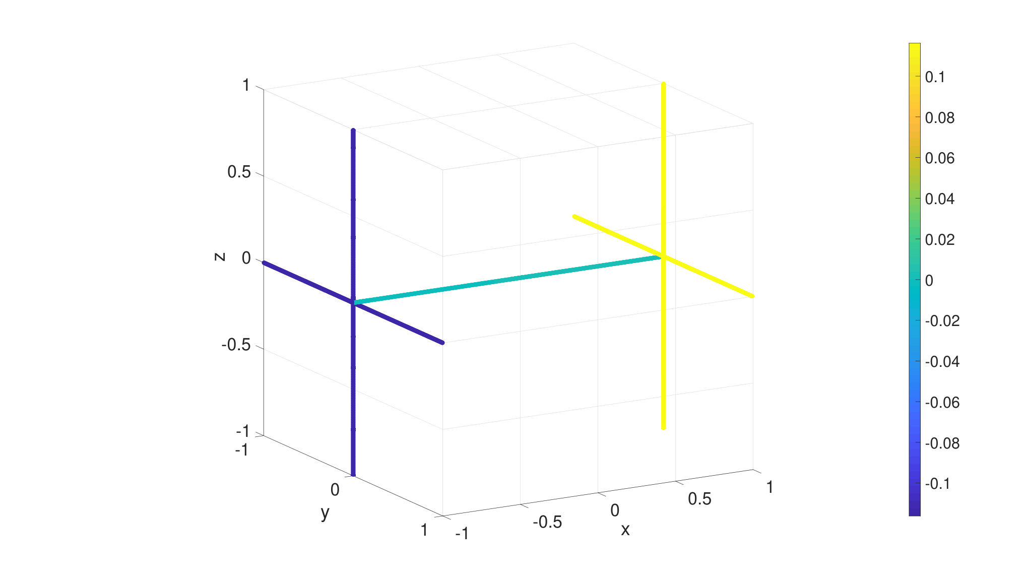
The global discrete solutions for the pressure head and the flux are presented in Figures 6.2(a) and 6.2(b), while the local solution on a fracture and a trace are given in Figures 6.2(c) and 6.2(d). In order to verify the discrete solution, the quantities , and are computed and verified to vanish within numerical accuracy for all domains, where and are the exact solutions for any domain and the subscript indicates a discrete solution. For the error in the flux variable the projection is required since the values of the discrete solution are not explicitly known inside a 3D or a 2D element.


Finally, this benchmark serves to show how a mixed VEM formulation (of any order) strongly imposes flux conservation and always displays a null flux mismatch up to machine precision. The flux chart in Figure 6.3 provides a visual example of this and exhibits how flux travels throughout the whole multidimensional system including boundary conditions (’BC’) and source/sink terms(’S’).
6.2 Problem 2: Embedded DFN with trace flow and finite inter-dimensional normal permeability
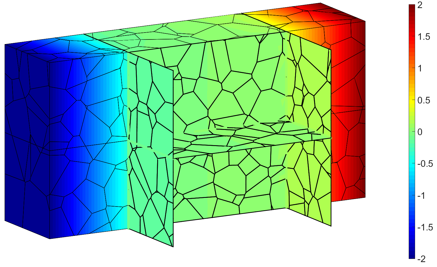
This problem was chosen to highlight the coupling between entities of different dimensions and to determine jumps in pressure that arise from finite normal permeability coefficients. In addition, lower dimensional objects are given much higher permeability values than their higher dimensional counterpart, resulting in a flow distribution that favours traces over fractures, and fractures over matrix. The problem consists of a 3D domain , 4 fractures () that give rise to 5 traces () that intersect in two points (). The notation and geometry are shown in Figure 6.4(a). Note that trace begins and ends precisely on the surface of and respectively. Data for this problem is as follows:
Boundary conditions are taken as a fixed pressure on and on . Homogeneous Neumann boundary conditions are imposed on all other boundaries for all entities. The problem was solved using RT2-VEM elements and a polyhedral mesh as detailed in Table 6.2.
| Element Type | #Elements | #3D DOFs | #2D DOFs | #1D DOFs | #0D DOFs | ||||||
| 3D | 2D | 1D | 0D | Flux | Pressure | Flux | Pressure | Flux | Pressure | Pressure | |
| RT2-VEM | 869 | 315 | 51 | 2 | 7194 | 48244 | 5391 | 1890 | 162 | 153 | 2 |
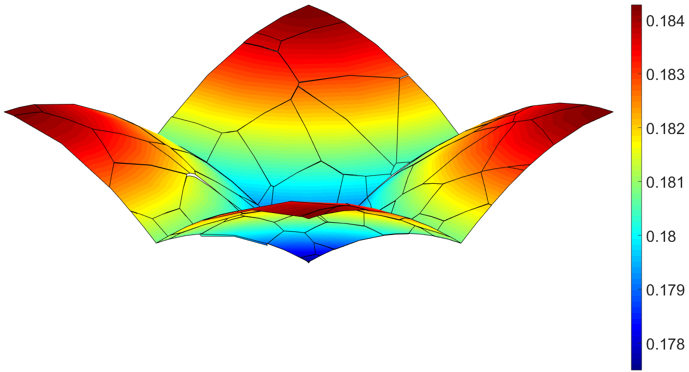
The obtained results present clearly noticeable jumps in pressure (see Figure 6.4(b)), as seen across and and . The effect of the finite interdimensional permeability in the velocity field is clear: it penalizes flux exchange since any non-zero flux exchange results in a drop of pressure inversely proportional to the normal permeability. For this reason, the velocity field in the mid part of the rock matrix is not entirely negligible (Figure 6.5(a)) despite the much higher permeability of the fractures and specially the traces, which represent a much more favourable path between entry and exit point. A second computation is provided as a comparison in which global continuity is imposed (i.e. infinite normal permeability) while keeping all other parameters the same. In this case, the aforementioned effect does not occur and the flow path is clearly dominated by the lower dimension entities (specially ), resulting in an almost vanishing flux in the mid section of the rock matrix and on fractures and (Figure 6.5(b)). Another consequence of global continuity is a difference in the total flux through the system. Since Dirichlet boundary conditions are imposed, incoming flux is dependent on the permeability parameters of the problem and the computed incoming fluxes are and for the finite permeability and global continuity situations respectively. As expected, global pressure continuity across dimensions provides a more favourable flow path, thus the global domain is more permeable resulting in larger flux values. Pressure head in the 1D trace network is given in Figure 6.6(a) showing pressure jumps across trace intersections. Finally, discrete solutions for pressure head and velocity field on fracture are shown in Figures 6.6(b) and 6.6(c).

6.3 Problem 3: Realistic embedded 16 fracture DFN
In this problem a 16 fracture DFN containing 38 traces and 15 intersections is embedded into a matrix of domain is as shown in Figure 6.7(a), where fractures are shaded and traces are depicted in red. Boundary conditions for the matrix consist of a constant unitary incoming flux on face , homogeneous Dirichlet on face and homogeneous Neumann (no-flux condition) on all remaining faces. For the DFN and the trace network, no-flux condition is imposed on all boundaries. There are neither source nor sink terms, and the given parameters are as follows:
Note that normal permeability between matrix and fractures is finite and therefore pressure head will not be globally continuous. In particular, fractures , and (whose boundaries are depicted in a darker shade) have very low normal permeability and effectively act as flow barriers.
The starting point for the discretization is a polyhedral mesh comprised of cubic elements, which, after successive fracture additions, results in the final mesh (Figure 6.7(b)) of polyhedral elements. Even though the number of fractures may seem low to discretize a network, which can amount to thousands of fractures, a small number of fractures can provide a better appreciation of the numerical results. Furthermore, even in this relatively contained example, the demand for computational power is high. Besides that, the generation of the final globally conforming mesh that takes the fractures into account is challenging as well, resulting in a final mesh that contains a plethora of very badly shaped elements with many undesirable features such as: small angles, tiny faces, short edges, large discrepancies in size between adjacent elements, collapsing nodes, etc (See mesh details on Figure 6.7(b)). Nevertheless, it would be undoubtedly more computationally expensive to solve this problem with a Finite Element mesh made up of the usual shapes (tetrahedra, hexahedra, pyramids and wedges) that is globally conforming from the start. This is due to the fact that a mesh for that situation would require a very small element size to be of acceptable quality as well as some type of iterative procedure to obtain matching discretizations between 3D faces and 2D fractures. Furthermore, VEM has been shown to be very robust to mesh distortion and the resulting mesh can be readily handled by the method.


The problem was solved using RT0-VEM, BDM1-VEM, RT1-VEM, BDM2-VEM and RT2-VEM, whose discretization statistics are provided in Table 6.3. Note that since 3D RTk-VEM and BDMk-VEM elements of the same order have an equal number of face DOFs for the flux variable, they can both be used in conjunction with 2D RTk-VEM elements for the fractures. The saving in DOFs for BDM elements is due to a reduction of internal flux DOFs and a lower order approximation of the 3D pressure field.
| Element Type | #Elements | #3D DOFs | #2D DOFs | #1D DOFs | #0D DOFs | |||||||
|---|---|---|---|---|---|---|---|---|---|---|---|---|
| 3D | 2D | 1D | Flux | Pressure | Flux | Pressure | Flux | Pressure | Pressure | |||
| RT0 | RT0 | 2734 | 1845 | 289 | 11584 | 2734 | 4707 | 1845 | 371 | 289 | 15 | |
| BDM1 | RT1 | 2734 | 1845 | 289 | 42957 | 2734 | 14972 | 5538 | 659 | 578 | 15 | |
| RT1 | RT1 | 2734 | 1845 | 289 | 51159 | 10936 | 14972 | 5538 | 659 | 578 | 15 | |
| BDM2 | RT2 | 2734 | 1845 | 289 | 107786 | 10936 | 28919 | 11076 | 951 | 867 | 15 | |
| RT2 | RT2 | 2734 | 1845 | 289 | 124190 | 27340 | 28919 | 11076 | 951 | 867 | 15 | |
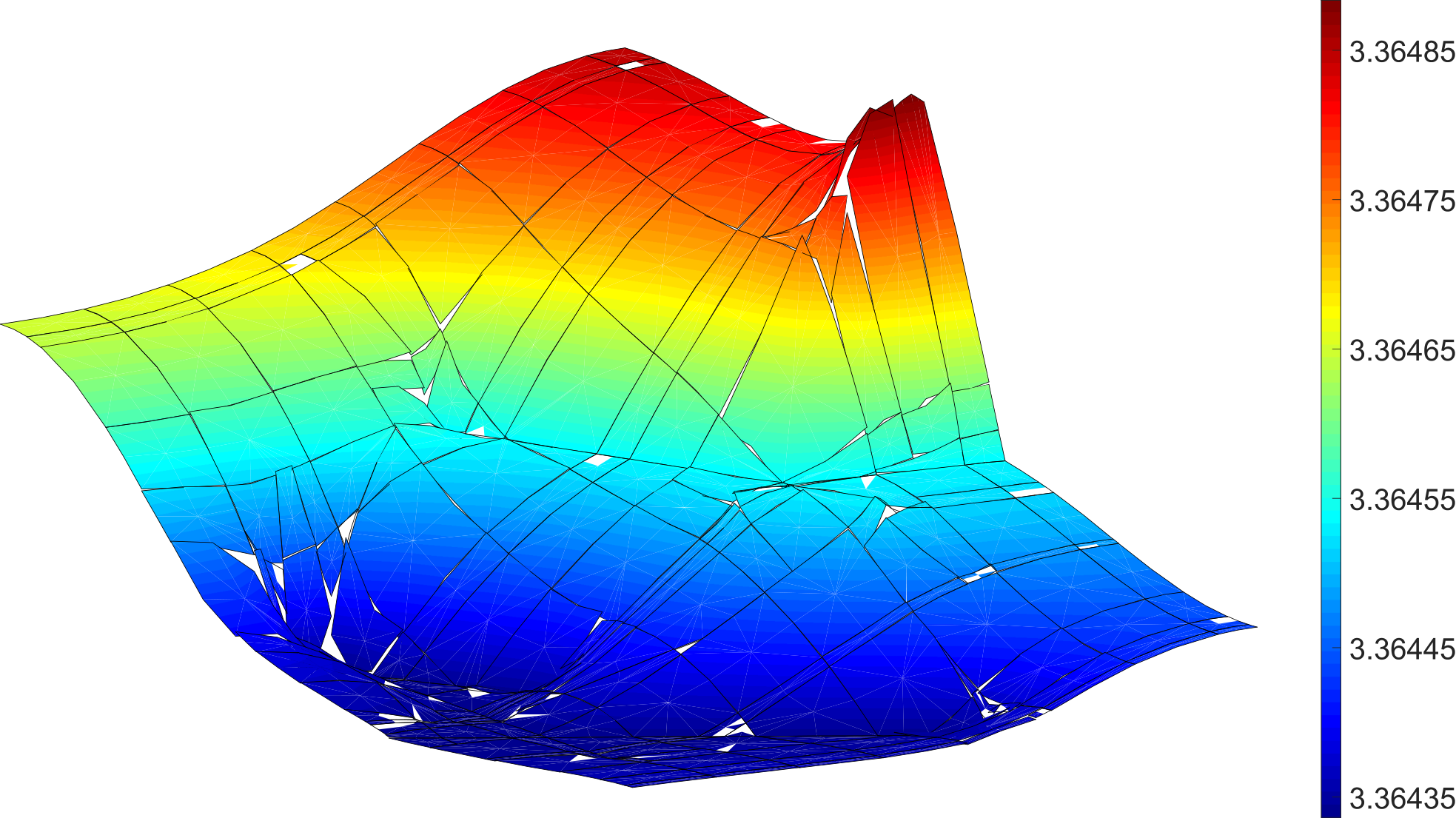
In the next Figures the results of the analysis are presented. The global pressure and the velocity field are shown in Figures 6.8 and 6.9, shown for the case of RT1-VEM elements, chosen for their linear approximation of both the flux and pressure variable. For the pressure, it can be clearly seen that the field is not globally continuous across fractures, most noticeably across those fractures with very low normal permeability, and that the small drop in pressure across the DFN is low due to the relatively high tangential permeability. The velocity field showcases the preferred flow paths in the multidimensional domain and the flux exchanges that take place. Despite not being a very dense, the trace network provides an advantageous flow path due to the high tangential permeability value and to the pressure continuity between fractures and traces as well as on trace intersections. The pressure and (normalized) velocity field for a particular fracture () presented in 6.10 for 2D RT0-, RT1- and RT2-VEM show a very strong qualitative agreement and a convergence towards and almost continuous local pressure field. Pressure values on an individual fracture are of course dependent on the global solution in the complete domain.


Some conclusions can be drawn from this problem. Firstly, the solution is highly dependent on the fracture distribution as expected. In fact, flux is greatest on fractures that provide the least effort path between boundaries with prescribed boundary conditions. Secondly, relative permeability between rock matrix and fractures has considerable influence on the result that can be clearly appreciated by the fact that only a very small drop in pressure is experienced across the whole DFN. On the other hand, taking into account the rock matrix in the model makes it significantly more expensive to solve, and should be avoided whenever the rock permeability is low enough such that the problem can be considered as mainly DFN-dominated. Thanks to global conservation of flux, results are very reliable for the flux variable even for low order elements. If 1D tangential permeability is high relative to the other domains, flux across the trace network is not negligible and should not be disregarded. A denser network of traces would further increase the influence of considering 1D elements in the solution. Finally, by inspecting the meshes used for computing the discrete solutions (obtained without any mesh improvement technique whatsoever) it can be seen that mixed VEM show great robustness and are affected very little by mesh quality.
7 Conclusions
A mixed Virtual Element formulation for multimensional problems for solving flow problems was explored in this work. A summary of the methodology as well as the main ideas of the method were included and details of its implementation were given a thorough treatment for an arbitrary discretization order. The crucial feature is the use of a polyhedral discretization with no initial requirement of mesh conformity. In fact, the rock matrix is given any mesh, on top of which the fractures that make up the DFN are added. Later, these fracture are incorporated to the global mesh by introducing cuts on the 3D elements. This would require some kind of remeshing-procedure for standard Finite Elements but that is not the case with VEM, than can handle the modified elements without any particular distinction over the original elements. Ultimately, a globally conforming polyhedral VEM mesh is obtained where faces, edges and vertices are automatically shared between inter-dimensional entities. Due to VEM’s robustness to mesh distortion, the numerical accuracy is not affected by the irregularity of the mesh.
The complete formulation for problems involving the combination of multidimensional entities was provided, where 2D elements representing embedded fractures are included in a 3D solid matrix. In addition, 1D elements representing traces given by fracture intersections were also included so as to take tangential trace flow into account. These traces constitute a trace network that requires flux balance and adequate pressure conditions on the points defined by traces intersection. Each interaction between entities of different dimensions results in flux exchanges and pressure jumps. One key aspect to highlight is that whereas the primal formulation guarantees continuity of pressure head (or pressure head jump in the case of non infinite permeability), the mixed formulation has the advantage of being completely mass-conservative by definition of the discrete spaces themselves. This is a more desirable characteristic in flux computations in many cases where the computed flow field is used as the underlying convection field to serve as input for another model (e.g. in transport problems).
Several numerical experiments were performed to assess the validity of the methodology. Starting with a problem with a known polynomial solution, it was shown that the exact solution is recovered within machine accuracy over meshes made up of arbitrary polyhedra. Afterwards, a multidimensional problem was solved to highlight the interactions between inter-dimensional entities and to evaluate the effects of finite inter-dimensional permeability over the flow field. Finally, a small yet realistic DFN was embedded in a 3D matrix for which the flow and pressure fields were determined and comparisons of discrete solutions were made between different interpolation orders.
It is straightforward to generalize the approach to second order elliptic problems. Time-dependent phenomena could be tackled as well and would follow standard procedure once the mass and stiffness matrix for the VEM discretization are obtained. From a computational point of view, the method shows potential for parallelization, since each dimension of the problem can be computed independently (even in parallel themselves) and the coupling between dimensions can be added once the respective stiffness matrices have been computed. However, 3D computations can be orders of magnitude slower than their 2- and 1-dimensional counterparts, mainly due to the much steeper increase in 3D DOFs for mesh refinement and increasing order of interpolation.
In conclusion, the arbitrary order mixed formulation Virtual Element Method presented here displays clear advantages in the study of geometrically complex hybrid dimensional flow problem mainly due to simpler meshing, easier implementation, strongly imposed mass conservation and accurate flux results.
Acknowledgments
A.B. and S.S. acknowledge the financial support of MIUR through the PRIN grant n. 201744KLJL and through the project “Dipartimenti di Eccellenza 2018-2022” (CUP E11G18000350001), and by INdAM-GNCS.
References
- [1] R. Ahmed, M. Edwards, S. Lamine, B. Huisman, and M. Pal, Control-volume distributed multi-point flux approximation coupled with a lower-dimensional fracture model, Journal of Computational Physics, 284 (2015), pp. 462 – 489.
- [2] O. Al-Hinai, S. Srinivasan, and M. F. Wheeler, Domain decomposition for flow in porous media with fractures, in SPE Reservoir Simulation Symposium 23-25 February 2013, Houston, Texas, USA, Society of Petroleum Engineers, 2015.
- [3] O. Al-Hinai, S. Srinivasan, and M. F. Wheeler, Mimetic finite differences for flow in fractures from microseismic data, in SPE Reservoir Simulation Symposium, Society of Petroleum Engineers, 2015.
- [4] Angot, Philippe, Boyer, Franck, and Hubert, Florence, Asymptotic and numerical modelling of flows in fractured porous media, ESAIM: M2AN, 43 (2009), pp. 239–275.
- [5] P. F. Antonietti, L. Formaggia, A. Scotti, M. Verani, and N. Verzott, Mimetic finite difference approximation of flows in fractured porous media, ESAIM: Mathematical Modelling and Numerical Analysis, 50 (2016), pp. 809–832.
- [6] E. Artioli, S. de Miranda, C. Lovadina, and L. Patruno, A stress/displacement Virtual Element method for plane elasticity problems, Computer Methods in Applied Mechanics and Engineering, 325 (2017), pp. 155 – 174.
- [7] L. Beirão da Veiga, F. Brezzi, A. Cangiani, G. Manzini, L. D. Marini, and A. Russo, Basic principles of Virtual Element methods, Math. Models and Methods in Applied Sciences, (2013).
- [8] L. Beirão da Veiga, F. Brezzi, L. D. Marini, and A. Russo, Mixed virtual element methods for general second order elliptic problems on polygonal meshes, ESAIM: Mathematical Modelling and Numerical Analysis, 50 (2016), pp. 727–747.
- [9] L. Beirão da Veiga, F. Brezzi, L. D. Marini, and A. Russo, H(div) and H(curl)-conforming virtual element methods, Numer. Math., 133 (2016), pp. 303–332.
- [10] M. F. Benedetto, The mixed virtual element formulation for three dimensional problems with embedded planes, Master’s Thesis, (2018).
- [11] M. F. Benedetto, S. Berrone, and A. Borio, The Virtual Element Method for underground flow simulations in fractured media, in Advances in Discretization Methods, vol. 12 of SEMA SIMAI Springer Series, Springer International Publishing, Switzerland, 2016, pp. 167–186.
- [12] M. F. Benedetto, S. Berrone, S. Pieraccini, and S. Scialò, The virtual element method for discrete fracture network simulations, Comput. Methods Appl. Mech. Engrg., 280 (2014), pp. 135 – 156.
- [13] M. F. Benedetto, S. Berrone, and S. Scialò, A globally conforming method for solving flow in discrete fracture networks using the virtual element method, Finite Elements in Analysis and Design, 109 (2016), pp. 23 – 36.
- [14] M. F. Benedetto, A. Borio, and S. Scialò, Mixed virtual elements for discrete fracture network simulations, Finite Elements in Analysis and Design, 134 (2017), pp. 55 – 67.
- [15] S. Berrone and A. Borio, Orthogonal polynomials in badly shaped polygonal elements for the Virtual Element Method, Finite Elements in Analysis & Design, 129 (2017), pp. 14–31.
- [16] S. Berrone and A. Borio, Orthogonal polynomials in badly shaped polygonal elements for the virtual element method, Finite Elements in Analysis and Design, 129 (2017), pp. 14 – 31.
- [17] S. Berrone, A. Borio, C. Fidelibus, S. Pieraccini, S. Scialò, and F. Vicini, Advanced computation of steady-state fluid flow in discrete fracture-matrix models: Fem–bem and vem–vem fracture-block coupling, GEM - International Journal on Geomathematics, 9 (2018), pp. 377–399.
- [18] S. Berrone, C. Fidelibus, S. Pieraccini, S. Scialò, and F. Vicini, Unsteady advection-diffusion simulations in complex Discrete Fracture Networks with an optimization approach, Journal of Hydrology, 566 (2018), pp. 332–345.
- [19] S. Berrone, S. Pieraccini, and S. Scialò, Flow simulations in porous media with immersed intersecting fractures, Journal of Computational Physics, 345 (2017), pp. 768 – 791.
- [20] S. Berrone, S. Scialò, and F. Vicini, Parallel meshing, discretization and computation of flow in massive Discrete Fracture Networks, SIAM J. Sci. Comput., 41 (2019), pp. C317–C338.
- [21] W. Boon, J. Nordbotten, and I. Yotov, Robust discretization of flow in fractured porous media, SIAM Journal on Numerical Analysis, 56 (2018), pp. 2203–2233.
- [22] K. Brenner, M. Groza, C. Guichard, G. Lebeau, and R. Masson, Gradient discretization of hybrid dimensional Darcy flows in fractured porous media, Numerische Mathematik, 134 (2016), pp. 569–609.
- [23] Brezzi, F., Falk, Richard S., and Donatella Marini, L., Basic principles of mixed virtual element methods, ESAIM: M2AN, 48 (2014), pp. 1227–1240.
- [24] F. Chave, D. Di Pietro, and L. Formaggia, A hybrid high-order method for darcy flows in fractured porous media, SIAM Journal on Scientific Computing, 40 (2018), pp. A1063–A1094.
- [25] Z. Chen, G. Huan, and Y. Ma, Computational Methods for Multiphase Flows in Porous Media, SIAM, Philadelphia, PA, USA, 2006.
- [26] J. Coulet, I. Faille, V. Girault, N. Guy, and F. Nataf, A fully coupled scheme using virtual element method and finite volume for poroelasticity, Computational Geosciences, (2019).
- [27] E. Cáceres and G. N. Gatica, A mixed virtual element method for the pseudostress–velocity formulation of the stokes problem, IMA Journal of Numerical Analysis, 37 (2017), pp. 296–331.
- [28] E. Cáceres, G. N. Gatica, and F. A. Sequeira, A mixed virtual element method for the brinkman problem, Mathematical Models and Methods in Applied Sciences, 27 (2017), pp. 707–743.
- [29] , A mixed virtual element method for quasi-newtonian stokes flows, SIAM Journal on Numerical Analysis, 56 (2018), pp. 317–343.
- [30] L. B. da Veiga, F. Brezzi, L. D. Marini, and A. Russo, Virtual Element Implementation for General Elliptic Equations, Springer International Publishing, Cham, 2016, pp. 39–71.
- [31] D´Angelo, Carlo and Scotti, Anna, A mixed finite element method for darcy flow in fractured porous media with non-matching grids, ESAIM: M2AN, 46 (2012), pp. 465–489.
- [32] F. Dassi and S. Scacchi, Parallel solvers for virtual element discretizations of elliptic equations in mixed form, https://arxiv.org/abs/1901.02330, 00 (2019).
- [33] F. Dassi and G. Vacca, Bricks for the mixed high-order virtual element method: Projectors and differential operators, Applied Numerical Mathematics, (2019).
- [34] W. S. Dershowitz and C. Fidelibus, Derivation of equivalent pipe networks analogues for three-dimensional discrete fracture networks by the boundary element method, Water Resource Res., 35 (1999), pp. 2685–2691.
- [35] I. Faille, A. Fumagalli, J. Jaffré, and J. E. Roberts, Model reduction and discretization using hybrid finite volumes for flow in porous media containing faults, Computational Geosciences, 20 (2016), pp. 317–339.
- [36] C. Fidelibus, The 2d hydro-mechanically coupled response of a rock mass with fractures via a mixed BEM-FEM technique, International Journal for Numerical and Analytical Methods in Geomechanics, 31 (2007), pp. 1329–1348.
- [37] L. Formaggia, A. Fumagalli, A. Scotti, and P. Ruffo, A reduced model for Darcy’s problem in networks of fractures, ESAIM: Mathematical Modelling and Numerical Analysis, 48 (2014), pp. 1089–1116.
- [38] T.-P. Fries and T. Belytschko, The extended/generalized finite element method: an overview of the method and its applications, Internat. J. Numer. Methods Engrg., 84 (2010), pp. 253–304.
- [39] A. Fumagalli and E. Keilegavlen, Dual virtual element method for discrete fractures networks, SIAM Journal on Scientific Computing, 40 (2018), pp. B228–B258.
- [40] A. Fumagalli, E. Keilegavlen, and S. Scialò, Conforming, non-conforming and non-matching discretization couplings in discrete fracture network simulations, J. Comput. Phys., 376 (2019), pp. 694–712.
- [41] A. Fumagalli and A. Scotti, A numerical method for two-phase flow in fractured porous media with non-matching grids, Advances in Water Resources, 62 (2013), pp. 454 – 464.
- [42] Fumagalli, Alessio and Keilegavlen, Eirik, Dual virtual element methods for discrete fracture matrix models, Oil Gas Sci. Technol. - Rev. IFP Energies nouvelles, 74 (2019), p. 41.
- [43] M. Gentile, A. Sommariva, and M. Vianello, Polynomial interpolation and cubature over polygons, Journal of Computational and Applied Mathematics, 235 (2011), pp. 5232 – 5239.
- [44] H. Hajibeygi, D. Karvounis, and P. Jenny, A hierarchical fracture model for the iterative multiscale finite volume method, Journal of Computational Physics, 230 (2011), pp. 8729 – 8743.
- [45] J. D. Hyman, S. Karra, N. Makedonska, C. W. Gable, S. L. Painter, and H. S. Viswanathan, dfnworks: A discrete fracture network framework for modeling subsurface flow and transport, Computers & Geosciences, 84 (2015), pp. 10 – 19.
- [46] L. Li and S. H. Lee, Efficient Field-Scale Simulation of Black Oil in a Naturally Fractured Reservoir Through Discrete Fracture Networks and Homogenized Media, SPE Reservoir Evaluation & Engineering, 11 (2008).
- [47] K. Lipnikov, G. Manzini, and M. Shashkov, Mimetic finite difference method, Journal of Computational Physics, 257 (2014), pp. 1163–1227.
- [48] V. Martin, J. Jaffré, and J. Roberts, Modeling fractures and barriers as interfaces for flow in porous media, SIAM Journal on Scientific Computing, 26 (2005), pp. 1667–1691.
- [49] A. Moinfar, A. Varavei, K. Sepehrnoori, and R. Johns, Development of an Efficient Embedded Discrete Fracture Model for 3D Compositional Reservoir Simulation in Fractured Reservoirs, SPE Journal, 19 (2014).
- [50] S. P. Neuman, Trends, prospects and challenges in quantifying flow and transport through fractured rocks, Hydrogeol. J., 13 (2005), pp. 124–147.
- [51] T. D. Ngo, A. Fourno, and B. Noetinger, Modeling of transport processes through large-scale discrete fracture networks using conforming meshes and open-source software, Journal of Hydrology, 554 (2017), pp. 66 – 79.
- [52] B. Nœtinger, A quasi steady state method for solving transient Darcy flow in complex 3D fractured networks accounting for matrix to fracture flow, J. Comput. Phys., 283 (2015), pp. 205–223.
- [53] B. Nœtinger and N. Jarrige, A quasi steady state method for solving transient Darcy flow in complex 3D fractured networks, J. Comput. Phys., 231 (2012), pp. 23–38.
- [54] J. M. Nordbotten, W. M. Boon, A. Fumagalli, and E. Keilegavlen, Unified approach to discretization of flow in fractured porous media, Computational Geosciences, 23 (2019), pp. 225–237.
- [55] A. W. Nordqvist, Y. W. Tsang, C. F. Tsang, B. Dverstop, and J. Andersson, A variable aperture fracture network model for flow and transport in fractured rocks, Water Resource Res., 28 (1992), pp. 1703–1713.
- [56] G. Pichot, J. Erhel, and J. de Dreuzy, A generalized mixed hybrid mortar method for solving flow in stochastic discrete fracture networks, SIAM Journal on scientific computing, 34 (2012), pp. B86 – B105.
- [57] D. Qi and T. Hesketh, An analysis of upscaling techniques for reservoir simulation, Petroleum Science and Technology, 23 (2005), pp. 827–842.
- [58] T. Sandve, I. Berre, and J. Nordbotten, An efficient multi-point flux approximation method for discrete fracture–matrix simulations, Journal of Computational Physics, 231 (2012), pp. 3784 – 3800.
- [59] M. Vohralík, J. Maryška, and O. Severýn, Mixed and nonconforming finite element methods on a system of polygons, Applied Numerical Mathematics, 51 (2007), pp. 176–193.