跳到论文正文
W Papers独立论文阅读器 arXiv:2001.11133 论文正文 计算阅读时间 · 0%
引用这篇论文根据当前论文元数据生成,正式投稿前建议核对。


License: arXiv.org perpetual non-exclusive license
arXiv:2001.11133v1 [math.NA] 29 Jan 2020

Universal Algebraic Controllers and System Identification

Fredy Vides Address: Scientific Computing Innovation Center
School of Mathematics and Computer Science
Universidad Nacional Autónoma de Honduras
Tegucigalpa
Honduras
Email address: fredy.vides@unah.edu.hn
Date: August 11, 2026
Abstract.

In this document, some structured operator approximation theoretical methods for system identification of nearly eventually periodic systems, are presented. Let ℂn×m\mathbb{C}^{n\times m} denote the algebra of n×mn\times m complex matrices. Given ε>0\varepsilon>0, an arbitrary discrete-time dynamical system (Σ,𝒯)(\Sigma,\mathcal{T}) with state-space Σ\Sigma contained in the finite dimensional Hilbert space ℂn\mathbb{C}^{n}, whose state-transition map 𝒯:Σ×([0,∞)∩ℤ)→Σ\mathcal{T}:\Sigma\times([0,\infty)\cap\mathbb{Z})\to\Sigma is unknown or partially known, and needs to be determined based on some sampled data in a finite set Σ^={xt}1≤t≤m⊂Σ\hat{\Sigma}=\{x_{t}\}_{1\leq t\leq m}\subset\Sigma according to the rule 𝒯⁡(xt,1)=xt+1\mathcal{T}(x_{t},1)=x_{t+1} for each 1≤t≤m−11\leq t\leq m-1, and given x∈Σ^x\in\hat{\Sigma}. We study the solvability of the existence problems for two triples (p,A,φ)(p,A,\varphi) and (p,Aη,Φ)(p,A_{\eta},\Phi) determined by a polynomial p∈ℂ⁡[z]p\in\mathbb{C}[z] with deg⁡(p)≤m\deg(p)\leq m, a matrix root A∈ℂm×mA\in\mathbb{C}^{m\times m} and an approximate matrix root Aη∈ℂr×rA_{\eta}\in\mathbb{C}^{r\times r} of p⁡(z)=0p(z)=0 with r≤mr\leq m, two completely positive linear multiplicative maps φ:ℂm×m→ℂn×n\varphi:\mathbb{C}^{m\times m}\to\mathbb{C}^{n\times n} and Φ:ℂr×r→ℂn×n\Phi:\mathbb{C}^{r\times r}\to\mathbb{C}^{n\times n}, such that ‖𝒯⁡(x,t)−φ⁡(At)​x‖≤ε\|\mathcal{T}(x,t)-\varphi(A^{t})x\|\leq\varepsilon and ‖Φ⁡(Aηt)​x−φ⁡(At)​x‖≤ε\|\Phi(A_{\eta}^{t})x-\varphi(A^{t})x\|\leq\varepsilon, for each integer t≥1t\geq 1 such that ‖𝒯⁡(x,t)−y‖≤ε\|\mathcal{T}(x,t)-y\|\leq\varepsilon for some y∈Σ^y\in\hat{\Sigma}. Some numerical implementations of these techniques for the reduced-order predictive simulation of dynamical systems in continuum and quantum mechanics, are outlined.

Key words and phrases:
Completely positive linear map, system identification, state-transition map, eventually periodic system, covariance matrix.
2010 Mathematics Subject Classification
93B28, 47N70 (primary) and 93C57, 93B40 (secondary)

1. Introduction

In this document, we study some structured operator approximation problems that arise in the fields of system identification and model order reduction of large-scale dynamical systems.

The purpose of this document is to present some novel theoretical and computational techniques for constrained approximation and identification of data-driven systems in continuum and quantum mechanics. These systems can be interpreted as discrete-time systems that can be partially described by difference equations of the form

(1.1) Σ:{xt+1=S⁡(xt,t),t∈ℤ∩[0,∞)x1∈Σ⊆ℂn\Sigma:\left\{\begin{array}[]{l}x_{t+1}=S(x_{t},t),\penalty\ \penalty\ t\in\mathbb{Z}\cap[0,\infty)\\ x_{1}\in\Sigma\subseteq\mathbb{C}^{n}\end{array}\right.

where Σ⊆ℂn\Sigma\subseteq\mathbb{C}^{n} is the set of valid states for the system, and where S:ℂn×ℤ∩[0,∞)→ℂnS:\mathbb{C}^{n}\times\mathbb{Z}\cap[0,\infty)\to\mathbb{C}^{n} is some constrained map that is either partially known, or needs to be determined/discovered based on some (sampled) data {xt}1≤t≤N\{x_{t}\}_{1\leq t\leq N}, obtained in the form of data snapshots related to the system Σ\Sigma under study. One can also interpret the map SS in (1.1) using the transition block diagram (1.2) as a black-box device 𝔖\mathbf{\mathfrak{S}}, that needs to be determined in such a way that it can be used to transform the present state xtx_{t} into the next state xt+1x_{t+1}, according to (1.1).

(1.2) 𝔖\mathbf{\mathfrak{S}}xtx_{t}xt+1x_{t+1}

A state-transition map 𝒯\mathcal{T} for a data-driven system determined by (1.1) is a map 𝒯:Σ×ℤ∩[0,∞)→Σ\mathcal{T}:\Sigma\times\mathbb{Z}\cap[0,\infty)\to\Sigma that satisfies the recurrence relation xt+s=𝒯⁡(xt,s)x_{t+s}=\mathcal{T}(x_{t},s) for each xt∈Σx_{t}\in\Sigma that satisfies (1.1).

The discovery, simulation and predictive control of the evolution laws for systems of the form (1.1) are highly important in predictive data analytics, for models related to the automatic control of systems and processes in industry and engineering in the sense of [3, 1]. The motivation for the development of the techniques presented in this paper came from matrix approximation problems that arise in the fields of system identification and predictive data analytics in the sense of [9, 7]. We approach the solution to these problems by developing some data-driven operator-theoretic methods that combine ideas and results from C∗-representation theory and multivariate statistical analysis, in order to compute approximate matrix representations of state-transition maps 𝒯\mathcal{T} that one can use for system identification and model order reduction.

For the study reported in this document, we build on the abstract machinery introduced by Brockett and Willsky in [2] and by Farhood and Dullerud in [5]. Our contribution is the application of some of the operator theoretic techniques developed in [11] to extend the results in [2] to data-driven systems, we also develope new theoretical and computational procedures for the eventually periodic approximation of data-driven systems, using structured perturbations of covariance matrices, completely positive linear multiplicative maps, and discrete-time systems whose time evolution is approximately controlled by algebraic matrix sets.

In this document, special attention will be given to nearly eventually periodic systems, that is, systems that in some suitable sense that will be detailed in §3, approximately behave as an eventually periodic system in the sense of [5].

Although, on this paper we will focus on the solution of the theoretical problems related to the existence and computability of finite-state approximation of data-driven systems determined by data sequences described by (1.1), the constructive nature of the results presented in this document allows one to derive prototypical algorithms like the ones presented in §4.1. Some numerical implementations of this prototypical algorithms are presented in §4.2.

2. Preliminaries and Notation

Since in this study, the information about a given system is provided essentially by orbits (data sequences) in some valid state space Σ\Sigma, from here on, we will refer to data-driven systems of the form (1.1) in terms of sets or elements in a state space Σ\Sigma. Given a state-transition map 𝒯:Σ×ℤ∩[0,∞)→Σ\mathcal{T}:\Sigma\times\mathbb{Z}\cap[0,\infty)\to\Sigma corresponding to a data-driven system Σ\Sigma of the form (1.1) and given a state x∈Σx\in\Sigma, we will write 𝒯s​(x)\mathcal{T}_{s}(x) to denote the state determined by the operation 𝒯⁡(x,s)\mathcal{T}(x,s).

We will write ℤ+\mathbb{Z}^{+} to denote the set of positive integers ℤ∩[1,∞)\mathbb{Z}\cap[1,\infty). In this document the symbol ℂn×m\mathbb{C}^{n\times m} will denote the algebra of n×mn\times m complex matrices, and we will write 𝟏n\mathbf{1}_{n} to denote the identity matrix in ℂn×n\mathbb{C}^{n\times n} and 𝟎n,m\mathbf{0}_{n,m} to denote the zero matrix in ℂn×m\mathbb{C}^{n\times m}. From here on, given a matrix X∈ℂm×nX\in\mathbb{C}^{m\times n}, we will write X∗X^{\ast} to denote the conjugate transpose of XX determined by X∗=X⊤¯=[X¯j​i]X^{\ast}=\overline{X^{\top}}=[\overline{X}_{ji}] in ℂn×m\mathbb{C}^{n\times m}. We will represent vectors in ℂn\mathbb{C}^{n} as column matrices in ℂn×1\mathbb{C}^{n\times 1}.

Given x∈ℂnx\in\mathbb{C}^{n} we will write ‖x‖\|x\| to denote the norm induced by the usual inner product in the Hilbert space ℂn\mathbb{C}^{n} determined by ‖x‖=x∗​x=(∑j=1n|xj|2)1/2\|x\|=\sqrt{x^{\ast}x}=(\sum_{j=1}^{n}|x_{j}|^{2})^{1/2}. Given A∈ℂn×nA\in\mathbb{C}^{n\times n} we will write ‖A‖\|A\| to denote the spectral (operator) norm in ℂn×n\mathbb{C}^{n\times n} determined by ‖A‖=sup‖x‖=1‖A​x‖\|A\|=\sup_{\|x\|=1}\|Ax\|.

Given a matrix Z∈ℂn×nZ\in\mathbb{C}^{n\times n}, and a polynomial p∈ℂ⁡[z]p\in\mathbb{C}[z] over the complex numbers determined by the expression p⁡(z)=a0+a1​z+⋯+am​zmp(z)=a_{0}+a_{1}z+\cdots+a_{m}z^{m}, we will write p⁡(Z)p(Z) to denote the matrix in ℂn×n\mathbb{C}^{n\times n} defined by the expression p⁡(Z)=a0​𝟏n+a1​Z+⋯+am​Zmp(Z)=a_{0}\mathbf{1}_{n}+a_{1}Z+\cdots+a_{m}Z^{m}. We will write 𝒵m​(p)\mathcal{Z}_{m}(p) to denote the algebraic set of matrix roots of p⁡(x)=0p(x)=0 determined by the expression {X∈ℂm×m|p⁡(X)=𝟎n,n}\{X\in\mathbb{C}^{m\times m}\penalty\ |\penalty\ p(X)=\mathbf{0}_{n,n}\}, and given ε>0\varepsilon>0 we will write 𝒵m,ε​(p)\mathcal{Z}_{m,\varepsilon}(p) to denote the set of ε\varepsilon-approximate matrix roots of p⁡(x)=0p(x)=0 determined by the expression {X∈ℂm×m|‖p⁡(X)‖≤ε}\{X\in\mathbb{C}^{m\times m}\penalty\ |\penalty\ \|p(X)\|\leq\varepsilon\}

Given ε>0\varepsilon>0 and A∈ℂn×nA\in\mathbb{C}^{n\times n}, we will write σε​(A)\sigma_{\varepsilon}(A) to denote the ε\varepsilon-pseudospectrum of AA, that by [10, Theorem 2.1] is equivalent to the set of z∈ℂz\in\mathbb{C} such that

(2.1) ‖(z​𝟏n−A)​v‖<ε\|(z\mathbf{1}_{n}-A)v\|<\varepsilon

for some v∈ℂnv\in\mathbb{C}^{n} with ‖v‖=1\|v\|=1.

In this document we will write e^j,n\hat{e}_{j,n} to denote the matrices in ℂn×1\mathbb{C}^{n\times 1} representing the canonical basis of ℂn\mathbb{C}^{n} (the jj-column of the n×nn\times n identity matrix), that are determined by the expression

(2.2) e^j,n=[δ1,jδ2,j⋯δn−1,jδn,j]⊤\hat{e}_{j,n}=\begin{bmatrix}\delta_{1,j}&\delta_{2,j}&\cdots&\delta_{n-1,j}&\delta_{n,j}\end{bmatrix}^{\top}

for each 1≤j≤n1\leq j\leq n, where δk,j\delta_{k,j} is the Kronecker delta determined by the expression.

(2.3) δk,j={1,k=j0,k≠j\delta_{k,j}=\left\{\begin{array}[]{l}1,\>\>k=j\\ 0,\>\>k\neq j\end{array}\right.

We will write 𝐞n\mathbf{e}_{n} to denote the vector in ℂn\mathbb{C}^{n} with all of its components equal to 1. Given a vector x∈ℂnx\in\mathbb{C}^{n} we will write μ⁡(x)\mu(x) and σ^​(x)\hat{\sigma}(x) to denote the mean and standard deviation of xx, respectively, with μ⁡(x)\mu(x) and σ^​(x)\hat{\sigma}(x) defined by the following expressions.

(2.4) μ⁡(x)\displaystyle\mu(x) =1n​𝐞n∗​x\displaystyle=\frac{1}{n}\mathbf{e}_{n}^{\ast}x
(2.5) σ^​(x)\displaystyle\hat{\sigma}(x) =1n−1​‖x−μ⁡(x)​𝐞n‖\displaystyle=\frac{1}{\sqrt{n-1}}\|x-\mu(x)\mathbf{e}_{n}\|

Given a data matrix X∈ℂN×rX\in\mathbb{C}^{N\times r} with N≥2N\geq 2, we will write cov⁡(X)\mathrm{cov}(X) to denote the covariance matrix of XX in ℂr×r\mathbb{C}^{r\times r} defined by the expression.

(2.6) cov⁡(X)=1N−1​(X−1N​𝐞N​𝐞N∗​X)∗​(X−1N​𝐞N​𝐞N∗​X)\mathrm{cov}(X)=\frac{1}{N-1}\left(X-\frac{1}{N}\mathbf{e}_{N}\mathbf{e}_{N}^{\ast}X\right)^{\ast}\left(X-\frac{1}{N}\mathbf{e}_{N}\mathbf{e}_{N}^{\ast}X\right)

We will write that a matrix A∈ℂm×nA\in\mathbb{C}^{m\times n} is a (0,1)(0,1)-matrix if AA is an integer matrix in which each element is a 00 or 11.

3. Universal Algebraic Controllers

We will say that an orbit {xt}t≥1⊆Σ⊆ℂn\{x_{t}\}_{t\geq 1}\subseteq\Sigma\subseteq\mathbb{C}^{n} of a data-driven system Σ\Sigma is nearly eventually periodic (NEP), if for any ε>0\varepsilon>0 there are two integers T′≥1T^{\prime}\geq 1, τ′≥0\tau^{\prime}\geq 0, and a vector sequence {x^t}t≥1⊂ℂn\{\hat{x}_{t}\}_{t\geq 1}\subset\mathbb{C}^{n} of vectors such that.

(3.1) {x^1≠0‖x^t−xt‖≤εx^t+τ′+T′=x^t+τ′,t∈ℤ+\left\{\begin{array}[]{l}\hat{x}_{1}\neq 0\\ \|\hat{x}_{t}-x_{t}\|\leq\varepsilon\\ \hat{x}_{t+\tau^{\prime}+T^{\prime}}=\hat{x}_{t+\tau^{\prime}}\end{array}\right.,t\in\mathbb{Z}^{+}

For some fixed ε>0\varepsilon>0. Let us consider the smallest integers 0≤τ≤τ′0\leq\tau\leq\tau^{\prime} and 1≤T≤T′1\leq T\leq T^{\prime}, for which the relations (3.1) hold, the pair (τ,T)(\tau,T) will be called the ε\varepsilon-index of the orbit {xt}t≥1\{x_{t}\}_{t\geq 1}, and will be denoted by indε​({xt})\mathrm{ind}_{\varepsilon}(\{x_{t}\}).

We approach the solution to the system identification and predictive simulation problems for a data-driven system Σ\Sigma, combining some ideas and results from C∗-representation theory and multivariate statistical analysis, in order to compute approximate matrix representations of state-transition maps 𝒯\mathcal{T} that need to be determined based on some sampled-data in Σ\Sigma, that one can use for system identification and model order reduction.

More specifically, given ε>0\varepsilon>0, an arbitrary discrete-time dynamical system (Σ,𝒯)(\Sigma,\mathcal{T}) with state-space Σ\Sigma contained in the finite dimensional Hilbert space ℂn\mathbb{C}^{n}, whose state-transition map 𝒯:Σ×([0,∞)∩ℤ)→Σ\mathcal{T}:\Sigma\times([0,\infty)\cap\mathbb{Z})\to\Sigma is unknown or partially known, and needs to be determined based on some sampled data in a finite set Σ^={xt}1≤t≤m⊂Σ\hat{\Sigma}=\{x_{t}\}_{1\leq t\leq m}\subset\Sigma according to the rule 𝒯⁡(xt,1)=xt+1\mathcal{T}(x_{t},1)=x_{t+1} for each 1≤t≤m−11\leq t\leq m-1, and given x∈Σ^x\in\hat{\Sigma}. We study the solvability of the existence problem for the triples (p,A,φ)(p,A,\varphi) and (p,Aη,Φ)(p,A_{\eta},\Phi) determined by a polynomial p∈ℂ⁡[z]p\in\mathbb{C}[z] with deg⁡(p)≤m\deg(p)\leq m, a matrix AA in the algebraic set 𝒵m​(p)⊂ℂm×m\mathcal{Z}_{m}(p)\subset\mathbb{C}^{m\times m}, a matrix AηA_{\eta} in the set 𝒵r,ε​(p)⊂ℂr×r\mathcal{Z}_{r,\varepsilon}(p)\subset\mathbb{C}^{r\times r} with r≤mr\leq m, a linear map φ:ℂm×m→ℂn×n\varphi:\mathbb{C}^{m\times m}\to\mathbb{C}^{n\times n}, and a completely positive linear multiplicative map Φ:𝒵r,ε​(p)→ℂn×n\Phi:\mathcal{Z}_{r,\varepsilon}(p)\to\mathbb{C}^{n\times n}, such that the following constraints are satisfied

(3.2) ‖𝒯t​(x)−φ⁡(At)​x‖≤ε\displaystyle\|\mathcal{T}_{t}(x)-\varphi(A^{t})x\|\leq\varepsilon
(3.3) ‖Φ⁡(Aηt)​x−φ⁡(At)​x‖≤ε\displaystyle\|\Phi(A_{\eta}^{t})x-\varphi(A^{t})x\|\leq\varepsilon

for each integer t≥1t\geq 1 such that ‖𝒯t​(x)−y‖≤ε\|\mathcal{T}_{t}(x)-y\|\leq\varepsilon for some y∈Σ^y\in\hat{\Sigma}. The triples (p,A,φ)(p,A,\varphi) and (p,Aη,Φ)(p,A_{\eta},\Phi) determined by the sampled data Σ^\hat{\Sigma}, the "initial point" x∈Σ^x\in\hat{\Sigma}, and error tolerance ε>0\varepsilon>0, will be called the cyclic and reduced order cyclic universal algebraic controllers UAC for the system Σ\Sigma with respect to the triple (Σ^,x,ε)(\hat{\Sigma},x,\varepsilon), respectively, and this relations will be represented using the expressions (p,A,φ)=𝔘ℭ​(Σ^,x,ε)(p,A,\varphi)=\mathfrak{U_{C}}(\hat{\Sigma},x,\varepsilon) and (p,Aη,Φ)=𝔘ℜ​ℭ​(Σ^,x,ε)(p,A_{\eta},\Phi)=\mathfrak{U_{RC}}(\hat{\Sigma},x,\varepsilon).

Remark 3.1.

Given some sampled data Σ^={x1,x~2,…,x~N}\hat{\Sigma}=\{x_{1},\tilde{x}_{2},\ldots,\tilde{x}_{N}\} in an orbit {xt}t≥1\{x_{t}\}_{t\geq 1} of a NEP data-driven system Σ\Sigma determined by (1.1), without loss of generality we can decompose the computation of the UAC (p,A,φ)=𝔘ℭ​(Σ^,x,ε)(p,A,\varphi)=\mathfrak{U_{C}}(\hat{\Sigma},x,\varepsilon) and (p,Aη,Φ)=𝔘ℜ​ℭ​(Σ^,x,ε)(p,A_{\eta},\Phi)=\mathfrak{U_{RC}}(\hat{\Sigma},x,\varepsilon) as follows.

  1. 3.1.1

    Estimate (s,T)=indε​({xt})(s,T)=\mathrm{ind}_{\varepsilon}(\{x_{t}\}) based on Σ^={xt}1≤t≤N\hat{\Sigma}=\{x_{t}\}_{1\leq t\leq N} and set p⁡(z)=zs+T−zsp(z)=z^{s+T}-z^{s} 

  2. 3.1.2

    Compute A∈𝒵m​(p)A\in\mathcal{Z}_{m}(p) and a completely positive linear multiplicative map φ:ℂm×m→ℂn×n\varphi:\mathbb{C}^{m\times m}\to\mathbb{C}^{n\times n} that satisfy (3.2) 

  3. 3.1.3

    Compute Aη∈𝒵r,ε​(p)A_{\eta}\in\mathcal{Z}_{r,\varepsilon}(p) with r≤mr\leq m and a completely positive linear multiplicative map Φ:ℂr×r→ℂn×n\Phi:\mathbb{C}^{r\times r}\to\mathbb{C}^{n\times n} that satisfy (3.3) 

In this document, the maps φ:ℂm×m→ℂn×n\varphi:\mathbb{C}^{m\times m}\to\mathbb{C}^{n\times n} and Φ:ℂm×m→ℂn×n\Phi:\mathbb{C}^{m\times m}\to\mathbb{C}^{n\times n} determined by the UAC of the system Σ\Sigma, will be called the cyclic realization (CR) and the reduced cyclic realization (RCR) of the system Σ\Sigma, respectively.

We will now study the three steps in remark 3.1 that are involved in the computation of the unversal algebraic controllers of a data-driven system Σ\Sigma.

3.1. ε\varepsilon-Indices and nearly eventually periodic orbits

Given ε>0\varepsilon>0 and some sampled-data {x~t}t=1N\{\tilde{x}_{t}\}_{t=1}^{N} from the orbit {xt}t≥1\{x_{t}\}_{t\geq 1} of a system Σ\Sigma. In order to estimate indε​({xt})\mathrm{ind}_{\varepsilon}(\{x_{t}\}) based on the sample {x~t}t=1N\{\tilde{x}_{t}\}_{t=1}^{N} we will derive a theoretical and computational method based on the covariance matrices defined in (2.6).

3.1.1. (0,1)(0,1)-matrices and eventual periodicity detection

Given ε>0\varepsilon>0 and some sampled-data {x~t}t=1N\{\tilde{x}_{t}\}_{t=1}^{N} from the orbit {xt}t≥1⊂ℂn\{x_{t}\}_{t\geq 1}\subset\mathbb{C}^{n} of a system Σ\Sigma, with n≥2n\geq 2. Let us consider the history data matrix X∈ℂn×NX\in\mathbb{C}^{n\times N} determined by the expression.

(3.4) X=[|||x1x2⋯xN|||]X=\begin{bmatrix}|&|&&|\\ x_{1}&x_{2}&\cdots&x_{N}\\ |&|&&|\end{bmatrix}

We will derive a data-driven structured perturbation result for cov⁡(X)\mathrm{cov}(X).

Lemma 3.2.

Given two columns from X∈ℂn×NX\in\mathbb{C}^{n\times N} in (3.4) with n≥2n\geq 2, let us set ε=‖xj−xk‖\varepsilon=\|x_{j}-x_{k}\|. If we denote by covj,k​(X)\mathrm{cov}_{j,k}(X) the j​kjk entry of cov⁡(X)\mathrm{cov}(X), we will have that covj,k​(X)\mathrm{cov}_{j,k}(X) satisfies the following constraint.

(3.5) |covk,j​(X)−σ^​(xj)2|≤2​σ^​(xj)n−1​ε\left|\mathrm{cov}_{k,j}(X)-\hat{\sigma}(x_{j})^{2}\right|\leq\frac{2\hat{\sigma}(x_{j})}{\sqrt{n-1}}\varepsilon
Proof.

By definition of cov⁡(X)\mathrm{cov}(X) in (2.6) we have that.

covj,j​(X)=‖xj−μ⁡(xj)​𝐞n‖2n−1=σ^​(xj)2\mathrm{cov}_{j,j}(X)=\frac{\|x_{j}-\mu(x_{j})\mathbf{e}_{n}\|^{2}}{n-1}=\hat{\sigma}(x_{j})^{2}

Let us set p=xk−xjp=x_{k}-x_{j}, then xk=xj+px_{k}=x_{j}+p and this implies that.

covk,j​(X)\displaystyle\mathrm{cov}_{k,j}(X) =(xk−μ⁡(xk)​𝐞n)∗​(xj−μ⁡(xj)​𝐞n)n−1\displaystyle=\frac{(x_{k}-\mu(x_{k})\mathbf{e}_{n})^{\ast}(x_{j}-\mu(x_{j})\mathbf{e}_{n})}{n-1}
=((xj−μ⁡(xj)​𝐞n)+(p−μ⁡(p)​𝐞n))∗​(xj−μ⁡(xj)​𝐞n)n−1\displaystyle=\frac{((x_{j}-\mu(x_{j})\mathbf{e}_{n})+(p-\mu(p)\mathbf{e}_{n}))^{\ast}(x_{j}-\mu(x_{j})\mathbf{e}_{n})}{n-1}
=covj,j​(X)+(p−μ⁡(p)​𝐞n)∗​(xj−μ⁡(xj)​𝐞n)n−1\displaystyle=\mathrm{cov}_{j,j}(X)+\frac{(p-\mu(p)\mathbf{e}_{n})^{\ast}(x_{j}-\mu(x_{j})\mathbf{e}_{n})}{n-1}
(3.6) =σ^​(xj)2+(p−μ⁡(p)​𝐞n)∗​(xj−μ⁡(xj)​𝐞n)n−1\displaystyle=\hat{\sigma}(x_{j})^{2}+\frac{(p-\mu(p)\mathbf{e}_{n})^{\ast}(x_{j}-\mu(x_{j})\mathbf{e}_{n})}{n-1}

Since xk=xj+px_{k}=x_{j}+p and xj=xk−px_{j}=x_{k}-p we will also have that,

σ^​(xk)\displaystyle\hat{\sigma}(x_{k}) =1n−1​‖xj+p−μ⁡(xj+p)​𝐞n‖\displaystyle=\frac{1}{\sqrt{n-1}}\|x_{j}+p-\mu(x_{j}+p)\mathbf{e}_{n}\|
≤1n−1​‖xj−μ⁡(xj)​𝐞n‖+1n−1​‖p−μ⁡(p)​𝐞n‖\displaystyle\leq\frac{1}{\sqrt{n-1}}\|x_{j}-\mu(x_{j})\mathbf{e}_{n}\|+\frac{1}{\sqrt{n-1}}\|p-\mu(p)\mathbf{e}_{n}\|
(3.7) =σ^​(xj)+σ^​(p)\displaystyle=\hat{\sigma}(x_{j})+\hat{\sigma}(p)

and similarly.

(3.8) σ^​(xj)≤σ^​(xk)+σ^​(p)\displaystyle\hat{\sigma}(x_{j})\leq\hat{\sigma}(x_{k})+\hat{\sigma}(p)

By (3.7) and (3.8) we will have that.

|σ^​(xj)−σ^​(xk)|\displaystyle|\hat{\sigma}(x_{j})-\hat{\sigma}(x_{k})| ≤σ^​(p)\displaystyle\leq\hat{\sigma}(p)
=1n−1​‖p+μ⁡(p)​𝐞n‖\displaystyle=\frac{1}{\sqrt{n-1}}\|p+\mu(p)\mathbf{e}_{n}\|
≤1n−1​(‖p‖+|μ⁡(p)|​‖𝐞n‖)\displaystyle\leq\frac{1}{\sqrt{n-1}}(\|p\|+|\mu(p)|\|\mathbf{e}_{n}\|)
=1n−1​(‖p‖+nn​|𝐞n∗​p|)\displaystyle=\frac{1}{\sqrt{n-1}}(\|p\|+\frac{\sqrt{n}}{n}|\mathbf{e}_{n}^{\ast}p|)
≤1n−1​(‖p‖+nn​‖𝐞n‖​‖p‖)\displaystyle\leq\frac{1}{\sqrt{n-1}}(\|p\|+\frac{\sqrt{n}}{n}\|\mathbf{e}_{n}\|\|p\|)
(3.9) =2n−1​‖p‖=2​εn−1\displaystyle=\frac{2}{\sqrt{n-1}}\|p\|=\frac{2\varepsilon}{\sqrt{n-1}}

By (3.6) and (3.9) we will have that.

|covk,j​(X)−σ^​(xj)2|\displaystyle\left|\mathrm{cov}_{k,j}(X)-\hat{\sigma}(x_{j})^{2}\right| =|(p−μ⁡(p)​𝐞n)∗​(xj−μ⁡(xj)​𝐞n)n−1|\displaystyle=\left|\frac{(p-\mu(p)\mathbf{e}_{n})^{\ast}(x_{j}-\mu(x_{j})\mathbf{e}_{n})}{n-1}\right|
≤‖p−μ⁡(p)​𝐞n‖​‖xj−μ⁡(xj)​𝐞n‖n−1\displaystyle\leq\frac{\|p-\mu(p)\mathbf{e}_{n}\|\|x_{j}-\mu(x_{j})\mathbf{e}_{n}\|}{n-1}
(3.10) =σ^​(xj)​σ^​(p)≤2​σ^​(xj)n−1​ε\displaystyle=\hat{\sigma}(x_{j})\hat{\sigma}(p)\leq\frac{2\hat{\sigma}(x_{j})}{\sqrt{n-1}}\varepsilon

This completes the proof. ∎

Given δ>0\delta>0 and a data matrix XX in ℂn×N\mathbb{C}^{n\times N} with n≥2n\geq 2, let us write PD,δ​(X)P_{D,\delta}(X) to denote the (0,1)(0,1)-matrix PD,δ​(X)=[pk​j]P_{D,\delta}(X)=[p_{kj}] in ℂN×N\mathbb{C}^{N\times N} whose entries are defined by the expression.

(3.11) pk​j={1,when​|covk,j​(X)−σ^​(xj)2|≤δ​and​k≥j0,otherwisep_{kj}=\left\{\begin{array}[]{l}1,\>\>\mathrm{when}\>\>|\mathrm{cov}_{k,j}(X)-\hat{\sigma}(x_{j})^{2}|\leq\delta\>\mathrm{and}\>k\geq j\\ 0,\>\>\mathrm{otherwise}\end{array}\right.

We will derive some eventual periodicity detection methods based on the matrix PD,δ​(X)P_{D,\delta}(X). In order to do this, let us start by considering the matrix Ck,n∈ℂn×nC_{k,n}\in\mathbb{C}^{n\times n} determined by the expression.

(3.12) Ck,n=[000⋯δk,1100⋯δk,2010⋯δk,3⋱⋱⋱0⋯01δk,n]C_{k,n}=\begin{bmatrix}0&0&0&\cdots&\delta_{k,1}\\ 1&0&0&\cdots&\delta_{k,2}\\ 0&1&0&\cdots&\delta_{k,3}\\ \vdots&\ddots&\ddots&\ddots&\vdots\\ 0&\cdots&0&1&\delta_{k,n}\end{bmatrix}

We call Ck,n∈ℂn×nC_{k,n}\in\mathbb{C}^{n\times n} a Generic Cyclic Shift matrix or GCS in this document. It can be seen that a matrix Ck,n∈ℂn×nC_{k,n}\in\mathbb{C}^{n\times n} determined by (3.12) can be represented in the form.

(3.13) Ck,n=e^k,n​e^n,n∗+∑j=1n−1e^j+1,n​e^j,n∗C_{k,n}=\hat{e}_{k,n}\hat{e}_{n,n}^{\ast}+\sum_{j=1}^{n-1}\hat{e}_{j+1,n}\hat{e}_{j,n}^{\ast}
Lemma 3.3.

The GCS matrix Ck,n∈ℂn×nC_{k,n}\in\mathbb{C}^{n\times n} satisfies the following conditions:

  1. (a)

    Ck,n​e^j,n=e^j+1,n,  1≤j≤n−1C_{k,n}\hat{e}_{j,n}=\hat{e}_{j+1,n},\>\>1\leq j\leq n-1

  2. (b)

    Ck,n​e^j,n=e^k,n,j=nC_{k,n}\hat{e}_{j,n}=\hat{e}_{k,n},\>\>j=n

  3. (c)

    Ck,nn−Ck,nk−1=𝟎n,nC_{k,n}^{n}-C_{k,n}^{k-1}=\mathbf{0}_{n,n}

  4. (d)

    For any two integers s≥0s\geq 0 and T≥1T\geq 1

    (3.14) Cs+1,s+Ts+m​T​x=Cs+1,s+Ts​xC_{s+1,s+T}^{s+mT}x=C_{s+1,s+T}^{s}x

    for each integer m≥0m\geq 0 and each vector x∈ℂs+Tx\in\mathbb{C}^{s+T}.

  5. (e)

    If we define PS,s+1=∑j=s+1s+Te^j,s+T​e^j,s+T∗P_{S,{s+1}}=\sum_{j=s+1}^{s+T}\hat{e}_{j,s+T}\hat{e}_{j,s+T}^{\ast} then,

    (3.15) PC,s+12\displaystyle P_{C,s+1}^{2} =PC,s+T=PC,s+1∗\displaystyle=P_{C,s+T}=P_{C,s+1}^{\ast}
    (3.16) PC,s+1\displaystyle P_{C,s+1} =(PC,s+1​Cs+1,s+T​PC,s+1)T\displaystyle=(P_{C,s+1}C_{s+1,s+T}P_{C,s+1})^{T}
Proof.

By (2.3) and (3.13) we will have that.

Ck,n​e^j,n\displaystyle C_{k,n}\hat{e}_{j,n} =e^k,n​(e^n,n∗​e^j,n)+∑s=1n−1e^s+1,n​(e^s,n∗​e^j,n)\displaystyle=\hat{e}_{k,n}(\hat{e}^{\ast}_{n,n}\hat{e}_{j,n})+\sum_{s=1}^{n-1}\hat{e}_{s+1,n}(\hat{e}_{s,n}^{\ast}\hat{e}_{j,n})
=δn,j​e^k,n+∑s=1n−1δs,j​e^s+1,n\displaystyle=\delta_{n,j}\hat{e}_{k,n}+\sum_{s=1}^{n-1}\delta_{s,j}\hat{e}_{s+1,n}
={e^j+1,n,  1≤j≤n−1e^k,n,j=n\displaystyle=\left\{\begin{array}[]{l}\hat{e}_{j+1,n},\>\>1\leq j\leq n-1\\ \hat{e}_{k,n},\>\>j=n\end{array}\right.

It can be seen that the GCS matrix Ck,nC_{k,n} determined by (3.12) can be expressed in the form.

(3.17) Ck,n=[e^2,ne^3,ne^4,n⋯e^k,n]C_{k,n}=\begin{bmatrix}\hat{e}_{2,n}&\hat{e}_{3,n}&\hat{e}_{4,n}&\cdots&\hat{e}_{k,n}\end{bmatrix}

By (3.17) and elementary linear algebra we will have that Ck,nC_{k,n} is the companion matrix of the polynomial pk∈ℂ⁡[z]p_{k}\in\mathbb{C}[z] determined by the expression.

(3.18) pk​(z)=zn−zk−1p_{k}(z)=z^{n}-z^{k-1}

This means that each GCS Ck,n∈ℂn×nC_{k,n}\in\mathbb{C}^{n\times n} satisfies the equation.

(3.19) pk​(Ck,n)=Ck,nn−Ck,nk−1=𝟎n,np_{k}(C_{k,n})=C_{k,n}^{n}-C_{k,n}^{k-1}=\mathbf{0}_{n,n}

And this implies that.

(3.20) Ck,nn−(k−1)​Ck,nk−1=Ck,nn=Ck,nk−1C_{k,n}^{n-(k-1)}C_{k,n}^{k-1}=C_{k,n}^{n}=C_{k,n}^{k-1}

By (3.20) we will have that for any three integers m,s≥0m,s\geq 0 and T≥1T\geq 1, and for any x∈ℂs+Tx\in\mathbb{C}^{s+T} we will have that.

(3.21) Cs+1,s+T(s+m​T)​x=Cs+1,s+Tm​T​Cs+1,s+Ts​x=Cs+1,s+Ts​xC_{s+1,s+T}^{(s+mT)}x=C_{s+1,s+T}^{mT}C_{s+1,s+T}^{s}x=C_{s+1,s+T}^{s}x

By definition of PC,s+1P_{C,s+1} we will have that PC,s+1P_{C,s+1} is a block diagonal matrix of the form.

(3.22) PC,s+1=[𝟎s,s𝟎s,T𝟎T,s𝟏T]P_{C,s+1}=\begin{bmatrix}\mathbf{0}_{s,s}&\mathbf{0}_{s,T}\\ \mathbf{0}_{T,s}&\mathbf{1}_{T}\end{bmatrix}

By (3.22) it can be easily verified that PC,s+12=PC,s+TP_{C,s+1}^{2}=P_{C,s+T} and PC,s+1∗=PC,s+TP_{C,s+1}^{\ast}=P_{C,s+T}. By (3.17) and (3.22) we will have that.

(3.23) PC,s+1​Cs+1,s+T​PC,s+1=[𝟎s,s𝟎s,T𝟎T,sC1,T]P_{C,s+1}C_{s+1,s+T}P_{C,s+1}=\begin{bmatrix}\mathbf{0}_{s,s}&\mathbf{0}_{s,T}\\ \mathbf{0}_{T,s}&C_{1,T}\end{bmatrix}

By (c) we will have that C1,TT=𝟏TC_{1,T}^{T}=\mathbf{1}_{T}, and by (3.23) we will have that.

(PC,s+1​Cs+1,s+T​PC,s+1)T=[𝟎s,s𝟎s,T𝟎T,sC1,TT]=[𝟎s,s𝟎s,T𝟎T,s𝟏T]=PC,s+1(P_{C,s+1}C_{s+1,s+T}P_{C,s+1})^{T}=\begin{bmatrix}\mathbf{0}_{s,s}&\mathbf{0}_{s,T}\\ \mathbf{0}_{T,s}&C_{1,T}^{T}\end{bmatrix}=\begin{bmatrix}\mathbf{0}_{s,s}&\mathbf{0}_{s,T}\\ \mathbf{0}_{T,s}&\mathbf{1}_{T}\end{bmatrix}=P_{C,s+1}

This completes the proof. ∎

Lemma 3.4.

Given two integers s,Ts,T such that s≥0s\geq 0 and T≥1T\geq 1 and any matrix A∈𝒵n​(p)A\in\mathcal{Z}_{n}(p) for p⁡(z)=zs+T−zsp(z)=z^{s+T}-z^{s}, we will have that the system (Σ,𝒯)(\Sigma,\mathcal{T}) determined by the state-transition map 𝒯t=At\mathcal{T}_{t}=A^{t} is eventually periodic and for any x∈ℂn\{0}x\in\mathbb{C}^{n}\backslash\{0\} we will have that ind0​({𝒯t​(x)})=(s,T)\mathrm{ind}_{0}(\{\mathcal{T}_{t}(x)\})=(s,T).

Proof.

Since A∈𝒵n​(p)A\in\mathcal{Z}_{n}(p) we will have that As+T−As=𝟎s+T,s+TA^{s+T}-A^{s}=\mathbf{0}_{s+T,s+T}, this implies that As+T=AsA^{s+T}=A^{s} and that for any x∈ℂn\{0}x\in\mathbb{C}^{n}\backslash\{0\} and for each t∈ℤ+t\in\mathbb{Z}^{+}.

(3.24) 𝒯t+s+T​(x)=At+s+T​x=At​As+T​x=At​As​x=At+s​x=𝒯t+s​(x)\mathcal{T}_{t+s+T}(x)=A^{t+s+T}x=A^{t}A^{s+T}x=A^{t}A^{s}x=A^{t+s}x=\mathcal{T}_{t+s}(x)

By (3.24) we will have that if we set x~t=At​x\tilde{x}_{t}=A^{t}x for each t∈ℤ+t\in\mathbb{Z}^{+}, then x~t+s+T=x~t+s\tilde{x}_{t+s+T}=\tilde{x}_{t+s} and ‖𝒯t​(x)−x~t‖=0\|\mathcal{T}_{t}(x)-\tilde{x}_{t}\|=0, this implies that ind0​({x~t})=(s,T)\mathrm{ind}_{0}(\{\tilde{x}_{t}\})=(s,T). This completes the proof. ∎

Given ε>0\varepsilon>0 and some sampled data {x~t}1≤t≤N\{\tilde{x}_{t}\}_{1\leq t\leq N} from an orbit {xt}t≥1\{x_{t}\}_{t\geq 1} in the state space of a NEP system Σ\Sigma. We will write Indε​({x~t})=(s,T)\mathrm{Ind}_{\varepsilon}(\{\tilde{x}_{t}\})=(s,T), if there exist two integers s≥0s\geq 0 and T≥1T\geq 1 such that s+T≤N−1s+T\leq N-1 and for each k=1,…,N−(s+T)k=1,\ldots,N-(s+T) and each 1≤j≤s+T1\leq j\leq s+T.

(3.25) ‖[||x~k⋯x~k+s+T−1||]​Cs+1,s+T​e^j,s+T−[|x~k+j|]‖≤ε\left\|\begin{bmatrix}|&&|\\ \tilde{x}_{k}&\cdots&\tilde{x}_{k+s+T-1}\\ |&&|\end{bmatrix}C_{s+1,s+T}\hat{e}_{j,s+T}-\begin{bmatrix}|\\ \tilde{x}_{k+j}\\ |\end{bmatrix}\right\|\leq\varepsilon

We will call the pair (s,T)=Indε​({x~t})(s,T)=\mathrm{Ind}_{\varepsilon}(\{\tilde{x}_{t}\}) the sample index, the GCS matrix Cs+1,s+TC_{s+1,s+T} in (3.25) will be called the GCS factor of the system Σ\Sigma based on the sample {x~t}1≤t≤N\{\tilde{x}_{t}\}_{1\leq t\leq N}, and we will say that the sample {x~t}1≤t≤N\{\tilde{x}_{t}\}_{1\leq t\leq N} is meaningful if Indε​({x~t})=indε​({xt})\mathrm{Ind}_{\varepsilon}(\{\tilde{x}_{t}\})=\mathrm{ind}_{\varepsilon}(\{x_{t}\}), s+T≤N−1s+T\leq N-1 for (s,T)=Indε​({x~t})(s,T)=\mathrm{Ind}_{\varepsilon}(\{\tilde{x}_{t}\}), and ‖x~t−xt‖≤ε\|\tilde{x}_{t}-x_{t}\|\leq\varepsilon for each 1≤t≤s+T1\leq t\leq s+T.

Lemma 3.5.

Given ε>0\varepsilon>0 and some sampled data {x~t}1≤t≤N\{\tilde{x}_{t}\}_{1\leq t\leq N} from an orbit {xt}t≥1\{x_{t}\}_{t\geq 1} in the state space of a NEP system Σ⊆ℂn\Sigma\subseteq\mathbb{C}^{n} with n≥2n\geq 2. There is δ>0\delta>0 such that, if we set X=[x~1⋯x~N]X=[\tilde{x}_{1}\penalty\ \cdots\penalty\ \tilde{x}_{N}] and PD,δ​(X)k,jP_{D,\delta}(X)_{k,j} denotes the k,jk,j-entry of the matrix PD,δ​(X)P_{D,\delta}(X) defined in (3.11), then we will have that if Indε​({x~t})=(s,T)\mathrm{Ind}_{\varepsilon}(\{\tilde{x}_{t}\})=(s,T), then PD,δ​(X)q+m​T,q=1P_{D,\delta}(X)_{q+mT,q}=1 for each pair of integers qq and mm such that q≥sq\geq s, m≥0m\geq 0 and q+m​T≤Nq+mT\leq N.

Proof.

Since Indε​({x~t})=(s,T)\mathrm{Ind}_{\varepsilon}(\{\tilde{x}_{t}\})=(s,T), by (3.25) and by lemma 3.3 we will have that ‖x~q+m​T−xq‖≤ε\|\tilde{x}_{q+mT}-x_{q}\|\leq\varepsilon for each each pair of integers qq and mm such that q≥sq\geq s, m≥0m\geq 0 and q+m​T≤Nq+mT\leq N. By lemma 3.2 we will have that if we set δ=2​σ^​(xj)n−1​ε\delta=\frac{2\hat{\sigma}(x_{j})}{\sqrt{n-1}}\varepsilon, then |covk,j​(X)−σ^​(xj)2|≤δ|\mathrm{cov}_{k,j}(X)-\hat{\sigma}(x_{j})^{2}|\leq\delta by (3.5) and this implies that PD,δ​(X)q+m​T,q=1P_{D,\delta}(X)_{q+mT,q}=1 by (3.11). This completes the proof. ∎

The previous lemma allows one to read the pattern left in a given sample by the daynamical laws of an NEP system under study. In section §4.1 we will present some prototypical algorithms based on lemma 3.2 and lemma 3.5.

3.1.2. Controllers and algebraic matrix sets

Given ε>0\varepsilon>0, a polynomial p∈ℂ⁡[z]p\in\mathbb{C}[z], and a discrete-time dynamical system (Σ,𝒯)(\Sigma,\mathcal{T}) with Σ⊂ℂn\Sigma\subset\mathbb{C}^{n}, we will say that a family of orbits 𝒪(Σ)={{yt}t≥1⊂Σ}\mathcal{O}(\Sigma)=\{\{y_{t}\}_{t\geq 1}\subset\Sigma\} is ε\varepsilon-almost controlled by the algebraic matrix set 𝒵m​(p)\mathcal{Z}_{m}(p) for 1≤m≤n1\leq m\leq n, if for any orbit {xt}t≥1\{x_{t}\}_{t\geq 1} in 𝒪⁡(Σ)\mathcal{O}(\Sigma) there is a sample {x~t}1≤t≤N⊆{xt}t≥1\{\tilde{x}_{t}\}_{1\leq t\leq N}\subseteq\{x_{t}\}_{t\geq 1} with x~1=x1\tilde{x}_{1}=x_{1}, a matrix A∈𝒵N​(p)A\in\mathcal{Z}_{N}(p), and a vector y∈ℂNy\in\mathbb{C}^{N} such that for each integer t≥1t\geq 1 the following constraints are satisfied.

(3.26) ‖[||x~1⋯x~N||]​At​y−𝒯t​([|x1|])‖≤ε\left\|\begin{bmatrix}|&&|\\ \tilde{x}_{1}&\cdots&\tilde{x}_{N}\\ |&&|\end{bmatrix}A^{t}y-\mathcal{T}_{t}\left(\begin{bmatrix}|\\ x_{1}\\ |\end{bmatrix}\right)\right\|\leq\varepsilon

The normed relations in (3.26) provide an alternative algebraic approach to the computation by dynamic mode decomposition of the connecting matrix representation 𝕂\mathbb{K} of the Koopman operator in the sense of [8, §2] and [7], that is determined by some sampled-data {xt}t=1N\{x_{t}\}_{t=1}^{N} in an orbit of some data-driven system under study, according to the equations 𝕂​xt=xt+1\mathbb{K}{x}_{t}={x}_{t+1}, 1≤t≤N−11\leq t\leq N-1.

In this study we will focus on the algebraic matrix sets that almost control the dynamical behavior of NEP systems.

Theorem 3.6.

Given ε>0\varepsilon>0 and a meaningful sampled data {x~t}1≤t≤N\{\tilde{x}_{t}\}_{1\leq t\leq N} in an orbit {xt}t≥1\{x_{t}\}_{t\geq 1} of a NEP data-driven system Σ\Sigma, if Indε​({x~t})=(s,T)\mathrm{Ind}_{\varepsilon}(\{\tilde{x}_{t}\})=(s,T), then {xt}t≥1\{x_{t}\}_{t\geq 1} is 2​ε2\varepsilon-almost controlled by 𝒵s+T​(p)\mathcal{Z}_{s+T}(p) for p⁡(z)=zs+T−zsp(z)=z^{s+T}-z^{s}. Furthermore, the sequence {x~t}t≥1\{\tilde{x}_{t}\}_{t\geq 1} determined by the recurrence relations

(3.27) [|x~t+1|]=[||x1⋯xs+T||]​Cs+1,s+Tt​e^1,s+T\begin{bmatrix}|\\ \tilde{x}_{t+1}\\ |\end{bmatrix}=\begin{bmatrix}|&&|\\ x_{1}&\cdots&x_{s+T}\\ |&&|\end{bmatrix}C_{s+1,s+T}^{t}\hat{e}_{1,s+T}

with x~1=x1\tilde{x}_{1}=x_{1}, satisfies the condition Indε​({x~t})=(s,T)\mathrm{Ind}_{\varepsilon}(\{\tilde{x}_{t}\})=(s,T), and for each t∈ℤ+t\in\mathbb{Z}^{+} we have that ‖x~t−xt‖≤2​ε\|\tilde{x}_{t}-x_{t}\|\leq 2\varepsilon.

Proof.

Since {x~t}1≤t≤N\{\tilde{x}_{t}\}_{1\leq t\leq N} is meaningful and Indε​({x~t})=(s,T)\mathrm{Ind}_{\varepsilon}(\{\tilde{x}_{t}\})=(s,T), we will have that indε​({xt})=Indε​({x~t})\mathrm{ind}_{\varepsilon}(\{x_{t}\})=\mathrm{Ind}_{\varepsilon}(\{\tilde{x}_{t}\}) and ‖x~t−xt‖≤ε\|\tilde{x}_{t}-x_{t}\|\leq\varepsilon for each 1≤t≤s+T1\leq t\leq s+T, since indε​({xt})=(s,T)\mathrm{ind}_{\varepsilon}(\{x_{t}\})=(s,T) this implies that there is an eventually periodic sequence {x^t}t≥1\{\hat{x}_{t}\}_{t\geq 1} with x^1≠0\hat{x}_{1}\neq 0, such that for each t∈ℤ+t\in\mathbb{Z}^{+}.

(3.28) {‖x^t−xt‖≤εx^t+s=x^t+s+T\left\{\begin{array}[]{l}\|\hat{x}_{t}-x_{t}\|\leq\varepsilon\\ \hat{x}_{t+s}=\hat{x}_{t+s+T}\end{array}\right.

Let us consider the sequence {x~t}t≥1\{\tilde{x}_{t}\}_{t\geq 1} generated according to the following recurrence relations,

(3.29) [|x~t+1|]=[||x1⋯xs+T||]​Cs+1,s+Tt​e^1,s+T\begin{bmatrix}|\\ \tilde{x}_{t+1}\\ |\end{bmatrix}=\begin{bmatrix}|&&|\\ x_{1}&\cdots&x_{s+T}\\ |&&|\end{bmatrix}C_{s+1,s+T}^{t}\hat{e}_{1,s+T}

with x~1=x1\tilde{x}_{1}=x_{1}. By lemma 3.3 and by iterating on (3.25) we will have that for each integer t≥1t\geq 1.

(3.30) ‖[||x1⋯xs+T||]​Cs+1,s+Tt​e^1,s+T−[|x~t+1|]‖≤ε\left\|\begin{bmatrix}|&&|\\ x_{1}&\cdots&x_{s+T}\\ |&&|\end{bmatrix}C_{s+1,s+T}^{t}\hat{e}_{1,s+T}-\begin{bmatrix}|\\ \tilde{x}_{t+1}\\ |\end{bmatrix}\right\|\leq\varepsilon

By lemma 3.4 we will have that {x~t}t≥1\{\tilde{x}_{t}\}_{t\geq 1} is eventually periodic with ind0​({x~t})=(s,T)=ind0​({x^t})\mathrm{ind}_{0}(\{\tilde{x}_{t}\})=(s,T)=\mathrm{ind}_{0}(\{\hat{x}_{t}\}), and by (3.28) and (3.30) we will have that for each t∈ℤ+t\in\mathbb{Z}^{+}.

(3.31) ‖x^t−x~t‖≤max1≤t≤s+T​‖x^t−x~t‖=max1≤t≤s+T​‖x^t−xt‖≤ε\|\hat{x}_{t}-\tilde{x}_{t}\|\leq\mathrm{max}_{1\leq t\leq s+T}\|\hat{x}_{t}-\tilde{x}_{t}\|=\mathrm{max}_{1\leq t\leq s+T}\|\hat{x}_{t}-x_{t}\|\leq\varepsilon

By (3.28) and (3.31) we will have that for each t∈ℤ+t\in\mathbb{Z}^{+}.

(3.32) ‖xt−x~t‖≤‖xt−x^t‖+‖x^t−x~t‖≤2​ε\|x_{t}-\tilde{x}_{t}\|\leq\|x_{t}-\hat{x}_{t}\|+\|\hat{x}_{t}-\tilde{x}_{t}\|\leq 2\varepsilon

By lemma 3.3 we also have that for p⁡(z)=zs+T−zsp(z)=z^{s+T}-z^{s}, p⁡(Cs+1,s+T)=𝟎s+T,s+Tp(C_{s+1,s+T})=\mathbf{0}_{s+T,s+T} and this implies that.

(3.33) Cs+1,s+T∈𝒵s+T​(p)C_{s+1,s+T}\in\mathcal{Z}_{s+T}(p)

By (3.30) and (3.33) we have that {xt}t≥1\{x_{t}\}_{t\geq 1} is 2​ε2\varepsilon-almost controlled by 𝒵s+T​(p)\mathcal{Z}_{s+T}(p) for p⁡(z)=zs+T−zsp(z)=z^{s+T}-z^{s}. This completes the proof. ∎

3.2. Cyclic realizations

Given an orbit {xt}t≥1\{x_{t}\}_{t\geq 1} of a nearly eventually periodic data-driven system Σ\Sigma determined by (1.1), we will approach the computation of eventually periodic ε\varepsilon-approximate representations of the state-transition matrices {𝒯s}s≥1\{\mathcal{T}_{s}\}_{s\geq 1} that satisfy the equations 𝒯s​xt=xt+s\mathcal{T}_{s}x_{t}=x_{t+s}, by computing a discrete-time switched system Σ^\hat{\Sigma} (in the sense of [4, §4.2]) that is determined by the decomposition

(3.34) Σ^:{x^t+1=𝒯^t​x^1x^1=x1‖xt−x^t‖≤ε,t≥1\hat{\Sigma}:\left\{\begin{array}[]{l}\hat{x}_{t+1}=\hat{\mathcal{T}}_{t}\hat{x}_{1}\\ \hat{x}_{1}=x_{1}\\ \|x_{t}-\hat{x}_{t}\|\leq\varepsilon\end{array}\right.,t\geq 1

related to some available sampled data {x~t}1≤t≤N⊆Σ\{\tilde{x}_{t}\}_{1\leq t\leq N}\subseteq\Sigma, with Σ^⊆{x~t}1≤t≤N\hat{\Sigma}\subseteq\{\tilde{x}_{t}\}_{1\leq t\leq N} and where each matrix 𝒯t^\hat{\mathcal{T}_{t}} has to be determined based on the sampled data in Σ^\hat{\Sigma}.

Given some sampled data {x~t}t=1N\{\tilde{x}_{t}\}_{t=1}^{N} in an orbit of some data-driven system Σ\Sigma such that dim​span​({x~1,…,x~N−1})=N−1\mathrm{dim}\penalty\ \mathrm{span}(\{\tilde{x}_{1},\ldots,\tilde{x}_{N-1}\})=N-1. Let us write XN−1(0)X^{(0)}_{N-1} and XN−1(1)X^{(1)}_{N-1} to denote the data matrices in ℂn×(N−1)\mathbb{C}^{n\times(N-1)} determined by the expressions.

XN−1(0)\displaystyle X^{(0)}_{N-1} =[||x~1⋯x~N−1||]\displaystyle=\begin{bmatrix}|&&|\\ \tilde{x}_{1}&\cdots&\tilde{x}_{N-1}\\ |&&|\end{bmatrix}
(3.35) XN−1(1)\displaystyle X^{(1)}_{N-1} =[||x~2⋯x~N||]\displaystyle=\begin{bmatrix}|&&|\\ \tilde{x}_{2}&\cdots&\tilde{x}_{N}\\ |&&|\end{bmatrix}

Given a matrix A∈ℂ(N−1)×(N−1)A\in\mathbb{C}^{(N-1)\times(N-1)} that (approximately) solves the matrix equation.

(3.36) XN−1(1)=XN−1(0)​AX^{(1)}_{N-1}=X^{(0)}_{N-1}A

Let us consider the reduced singular value decomposition.

(3.37) XN−1(0)=U​S​VX^{(0)}_{N-1}=USV

with U∈ℂn×(N−1)U\in\mathbb{C}^{n\times{(N-1)}}, V∈ℂ(N−1)×(N−1)V\in\mathbb{C}^{(N-1)\times{(N-1)}} and S∈ℝ(N−1)×(N−1)S\in\mathbb{R}^{(N-1)\times(N-1)}. Given δ>0\delta>0, we will write XN−1,δ(0)X^{(0)}_{N-1,\delta} to denote the perturbed data matrix corresponding to XN−1(0)X^{(0)}_{N-1}, with reduced singular value decomposition

(3.38) XN−1,δ(0)=U​Sδ​VX^{(0)}_{N-1,\delta}=US_{\delta}V

where Sδ=[s^i​j]S_{\delta}=[\hat{s}_{ij}] is the diagonal matrix determined by the expression.

(3.39) s^j​j={sj​j,sj​j>0δ,sj​j=0\hat{s}_{jj}=\left\{\begin{array}[]{r}s_{jj}\>,\>\>s_{jj}>0\\ \delta\>,\>\>s_{jj}=0\end{array}\right.

Given an orbit {xt}t≥1\{x_{t}\}_{t\geq 1} in a NEP data-driven system Σ⊆ℂn\Sigma\subseteq\mathbb{C}^{n} and some meaningful sample {x~t}t=1N\{\tilde{x}_{t}\}_{t=1}^{N} from {xt}t≥1\{x_{t}\}_{t\geq 1} with Indε​({xt})=(s,T)\mathrm{Ind}_{\varepsilon}(\{x_{t}\})=(s,T) and s+T≤N−1s+T\leq N-1. We will study the existence of cyclic realizations Φ:ℂm×m→ℂn×n\Phi:\mathbb{C}^{m\times m}\to\mathbb{C}^{n\times n} for the nearly eventually periodic orbit {xt}t≥1\{x_{t}\}_{t\geq 1}, that satisfy (3.3).

Theorem 3.7.

Given ε>0\varepsilon>0, for any meaningful sampled data {x~t}1≤t≤N\{\tilde{x}_{t}\}_{1\leq t\leq N} from an orbit {xt}t≥1\{x_{t}\}_{t\geq 1} of a NEP data-driven system Σ⊆ℂn\Sigma\subseteq\mathbb{C}^{n}, there is δ>0\delta>0 such that if Indδ​({x~t})=(s,T)\mathrm{Ind}_{\delta}(\{\tilde{x}_{t}\})=(s,T), 1≤s+T≤N−11\leq s+T\leq N-1 and N≤nN\leq n, then there are two matrices A∈ℂn×nA\in\mathbb{C}^{n\times n} and U∈ℂn×(s+T)U\in\mathbb{C}^{n\times{(s+T)}} such that U∗​U=𝟏s+TU^{\ast}U=\mathbf{1}_{s+T}, A∈𝒵n,ε​(p)A\in\mathcal{Z}_{n,\varepsilon}(p) and U∗​A​U∈𝒵s+T,ε​(p)U^{\ast}AU\in\mathcal{Z}_{s+T,\varepsilon}(p) for p⁡(z)=zs+T+1−zs+1p(z)=z^{s+T+1}-z^{s+1}, and ‖xt+1−A​xt‖≤ε\|x_{t+1}-Ax_{t}\|\leq\varepsilon for each t∈ℤ+t\in\mathbb{Z}^{+}.

Proof.

Given ε>0\varepsilon>0. Let us consider any meaningful sampled data {x~t}1≤t≤N\{\tilde{x}_{t}\}_{1\leq t\leq N} from an orbit {xt}t≥1\{x_{t}\}_{t\geq 1} of a NEP data-driven system Σ⊆ℂn\Sigma\subseteq\mathbb{C}^{n} with N≤nN\leq n, choose ϑ>0\vartheta>0 such that Indϑ​({x~t})=(s,T)\mathrm{Ind}_{\vartheta}(\{\tilde{x}_{t}\})=(s,T) for some non-negative integers s,Ts,T such that 1≤s+T≤N−11\leq s+T\leq N-1. Let us consider the reduced singular value decomposition of the data matrix Xs+T(0)X^{(0)}_{s+T} corresponding to the sub-sample {x~t}t=1s+T+1\{\tilde{x}_{t}\}_{t=1}^{s+T+1} that is determined by the expression.

(3.40) Xs+T(0)=[||x~1⋯x~s+T||]=U​S​VX^{(0)}_{s+T}=\begin{bmatrix}|&&|\\ \tilde{x}_{1}&\cdots&\tilde{x}_{s+T}\\ |&&|\end{bmatrix}=USV

Let us consider the reduced singular value decomposition of the corresponding perturbed data matrix.

(3.41) Xs+T,ϑ(0)​[||x^1⋯x^s+T||]=U​Sϑ​VX^{(0)}_{s+T,\vartheta}\begin{bmatrix}|&&|\\ \hat{x}_{1}&\cdots&\hat{x}_{s+T}\\ |&&|\end{bmatrix}=US_{\vartheta}V

We will have that,

(3.42) rank⁡(Xs+T(0))≤rank⁡(Xs+T,ϑ(0))=rank⁡(Sϑ)=s+T\mathrm{rank}(X^{(0)}_{s+T})\leq\mathrm{rank}(X^{(0)}_{s+T,\vartheta})=\mathrm{rank}(S_{\vartheta})=s+T

and also that.

(3.43) ‖Xs+T(0)−Xs+T,ϑ(0)‖=‖U⁡(S−Sϑ)​V‖=‖S−Sϑ‖≤ϑ\|X^{(0)}_{s+T}-X^{(0)}_{s+T,\vartheta}\|=\|U(S-S_{\vartheta})V\|=\|S-S_{\vartheta}\|\leq\vartheta

By (3.42) we will have that Sϑ∈ℝ(s+T)×(s+T)S_{\vartheta}\in\mathbb{R}^{(s+T)\times(s+T)} is invertible, let us set.

(3.44) A=U​Sϑ​V​Cs+1,s+T​V∗​Sϑ−1​U∗A=US_{\vartheta}VC_{s+1,s+T}V^{\ast}S_{\vartheta}^{-1}U^{\ast}

Since U∗​U=𝟏nU^{\ast}U=\mathbf{1}_{n} we will have that for any X,Y∈ℂ(s+T)×(s+T)X,Y\in\mathbb{C}^{(s+T)\times(s+T)}, the linear map defined by the operation ϕ⁡(Y)=U​Y​U∗\phi(Y)=UYU^{\ast} satisfies the following condition.

(3.45) ϕ⁡(X​Y)=U​X​Y​U∗=U​X​U∗​U​Y​U∗=ϕ⁡(X)​ϕ​(Y)\phi(XY)=UXYU^{\ast}=UXU^{\ast}UYU^{\ast}=\phi(X)\phi(Y)

By (3.44) we will have that U∗​A​UU^{\ast}AU is similar to Cs+1,s+TC_{s+1,s+T}, this in turn implies that U∗​A​U∈𝒵s+T​(q)U^{\ast}AU\in\mathcal{Z}_{s+T}(q) for q⁡(z)=zs+T−zsq(z)=z^{s+T}-z^{s}, and this implies that U∗​A​U∈𝒵s+T​(p)U^{\ast}AU\in\mathcal{Z}_{s+T}(p) for p⁡(z)=zs+T+1−zs+1p(z)=z^{s+T+1}-z^{s+1}. By (3.45) we will have that.

(3.46) p⁡(A)=p⁡(ϕ⁡(U∗​A​U))=ϕ⁡(p⁡(U∗​A​U))=ϕ⁡(𝟎s+T,s+T)=𝟎n,np(A)=p(\phi(U^{\ast}AU))=\phi(p(U^{\ast}AU))=\phi(\mathbf{0}_{s+T,s+T})=\mathbf{0}_{n,n}

By lemma 3.3, (3.44) and (3.39) we will have that for each 1≤t≤s+T−11\leq t\leq s+T-1.

A​x^t\displaystyle A\hat{x}_{t} =A​Xs+T,ϑ(0)​e^t,s+T\displaystyle=AX^{(0)}_{s+T,\vartheta}\hat{e}_{t,s+T}
=U​Sϑ​V​Cs+1,s+T​V∗​Sϑ−1​U∗​U​Sϑ​V​e^t,s+T\displaystyle=US_{\vartheta}VC_{s+1,s+T}V^{\ast}S_{\vartheta}^{-1}U^{\ast}US_{\vartheta}V\hat{e}_{t,s+T}
(3.47) =U​Sϑ​V​Cs+1,s+T​e^t,s+T=Xs+T,ϑ(0)​e^t+1,s+T=x^t+1\displaystyle=US_{\vartheta}VC_{s+1,s+T}\hat{e}_{t,s+T}=X^{(0)}_{s+T,\vartheta}\hat{e}_{t+1,s+T}=\hat{x}_{t+1}

Let us consider the sequence {x^t}t≥1\{\hat{x}_{t}\}_{t\geq 1} generated by the recurrence raltions.

(3.48) {x^t+1=A​x^t,x^1=x1\left\{\begin{array}[]{l}\hat{x}_{t+1}=A\hat{x}_{t},\\ \hat{x}_{1}=x_{1}\end{array}\right.

Sice {x~t}t=1N−1\{\tilde{x}_{t}\}_{t=1}^{N-1} is meaningful and Indϑ​({x~t})=(s,T)\mathrm{Ind}_{\vartheta}(\{\tilde{x}_{t}\})=(s,T) we will have that ‖x~s+T+1−x~s+2‖≤ϑ\|\tilde{x}_{s+T+1}-\tilde{x}_{s+2}\|\leq\vartheta, this fact together with (3.47) will imply that for each 1≤t≤s+T1\leq t\leq s+T.

‖x~t+1−A​x~t‖\displaystyle\|\tilde{x}_{t+1}-A\tilde{x}_{t}\| ≤‖x~t+1−x^t+1‖+‖x^t+1−A​x^t‖+‖A​x^t−A​x~t‖\displaystyle\leq\|\tilde{x}_{t+1}-\hat{x}_{t+1}\|+\|\hat{x}_{t+1}-A\hat{x}_{t}\|+\|A\hat{x}_{t}-A\tilde{x}_{t}\|
(3.49) ≤ϑ+ϑ+‖A‖​ϑ=(‖A‖+2)​ϑ\displaystyle\leq\vartheta+\vartheta+\|A\|\vartheta=(\|A\|+2)\vartheta

By lemma 3.4 we will have that {x^t}t≥1\{\hat{x}_{t}\}_{t\geq 1} satisfies the condition indϑ​({x^t})=(s,T)\mathrm{ind}_{\vartheta}(\{\hat{x}_{t}\})=(s,T). Since indϑ​({xt})=(s,T)\mathrm{ind}_{\vartheta}(\{x_{t}\})=(s,T) we will have that there is an eventually periodic sequence {x~t}t≥1\{\tilde{x}_{t}\}_{t\geq 1} such that for each t∈ℤ+t\in\mathbb{Z}^{+}

(3.50) {‖xt−x~t‖≤ϑ,xt+s+T=xt+s\left\{\begin{array}[]{l}\|x_{t}-\tilde{x}_{t}\|\leq\vartheta,\\ x_{t+s+T}=x_{t+s}\end{array}\right.

By (3.49) and (3.50) we will have that.

‖xt+1−A​xt‖\displaystyle\|x_{t+1}-Ax_{t}\| ≤‖xt+1−x~t+1‖+‖x~t+1−x^t+1‖+‖x^t+1−A​x^t‖\displaystyle\leq\|x_{t+1}-\tilde{x}_{t+1}\|+\|\tilde{x}_{t+1}-\hat{x}_{t+1}\|+\|\hat{x}_{t+1}-A\hat{x}_{t}\|
+‖A​x^t−A​x~t‖+‖A​x~t−A​xt‖\displaystyle+\|A\hat{x}_{t}-A\tilde{x}_{t}\|+\|A\tilde{x}_{t}-Ax_{t}\|
≤‖xt+1−x~t+1‖+(‖A‖+1)​max1≤t≤s+T⁡(‖x~t−xt‖+‖xt−x^t‖)\displaystyle\leq\|x_{t+1}-\tilde{x}_{t+1}\|+(\|A\|+1)\max_{1\leq t\leq s+T}(\|\tilde{x}_{t}-x_{t}\|+\|x_{t}-\hat{x}_{t}\|)
+‖x^t+1−A​x^t‖+‖A‖​‖x~t−xt‖\displaystyle+\|\hat{x}_{t+1}-A\hat{x}_{t}\|+\|A\|\|\tilde{x}_{t}-x_{t}\|
(3.51) ≤ϑ+2​(‖A‖+1)​ϑ+ϑ+‖A‖​ϑ=(3​‖A‖+4)​ϑ\displaystyle\leq\vartheta+2(\|A\|+1)\vartheta+\vartheta+\|A\|\vartheta=(3\|A\|+4)\vartheta

Let us set δ=ϑ\delta=\vartheta and ε=(3​‖A‖+4)​ϑ\varepsilon=(3\|A\|+4)\vartheta. This completes the proof. ∎

Given ε>0\varepsilon>0 and some meaningful sample {x~t}t=1N\{\tilde{x}_{t}\}_{t=1}^{N} from an orbit {xt}t≥1\{x_{t}\}_{t\geq 1} of a NEP system Σ⊂ℂn\Sigma\subset\mathbb{C}^{n}. The matrices A,UA,U determined by theorem 3.7 will be called an approximate cyclic matrix realization for {xt}t≥1\{x_{t}\}_{t\geq 1} based on {x~t}t=1N\{\tilde{x}_{t}\}_{t=1}^{N}. This relation will be represented by the expression (A,U)=ℂ​𝕄​ℝ​({x~t},ε,δ)(A,U)=\mathbb{CMR}(\{\tilde{x}_{t}\},\varepsilon,\delta).

Corollary 3.8.

Given ε>0\varepsilon>0 and a meaningful sample {x~t}t=1N\{\tilde{x}_{t}\}_{t=1}^{N} from an orbit {xt}t≥1\{x_{t}\}_{t\geq 1} of a NEP system Σ⊂ℂn\Sigma\subset\mathbb{C}^{n}. There is δ>0\delta>0 such that if Indδ=(s,T)\mathrm{Ind}_{\delta}=(s,T) and s+T≤ns+T\leq n, then the problem (A,U)=ℂ​𝕄​ℝ​({x~t},ε,δ)(A,U)=\mathbb{CMR}(\{\tilde{x}_{t}\},\varepsilon,\delta) is solvable.

Proof.

A direct application of theorem 3.7. ∎

Lemma 3.9.

Given ε>0\varepsilon>0 and a polynomial p∈ℂ⁡[z]p\in\mathbb{C}[z], there is δ>0\delta>0 such that for any X,Y∈ℂn×nX,Y\in\mathbb{C}^{n\times n} such that ‖X‖≤2\|X\|\leq 2, ‖p⁡(X)‖≤δ\|p(X)\|\leq\delta and ‖X−Y‖≤δ\|X-Y\|\leq\delta, we have that ‖p⁡(Y)‖≤ε\|p(Y)\|\leq\varepsilon.

Proof.

Let us set.

(3.52) δ=max⁡{‖p⁡(X)‖,‖X−Y‖}\delta=\max\left\{\|p(X)\|,\|X-Y\|\right\}

Since p∈ℂ⁡[z]p\in\mathbb{C}[z] we will have that p(z)=a0+a1z+⋯anznp(z)=a_{0}+a_{1}z+\cdots a_{n}z^{n} for some a0,…,an∈ℂa_{0},\ldots,a_{n}\in\mathbb{C}. By (3.52) and by [6, Theorem 6.1.10] we will have that,

‖p⁡(Y)‖\displaystyle\|p(Y)\| =‖p⁡(X+(Y−X))−p⁡(X)+p⁡(X)‖\displaystyle=\|p(X+(Y-X))-p(X)+p(X)\|
≤‖p⁡(X+(Y−X))−p⁡(X)‖+‖p⁡(X)‖\displaystyle\leq\|p(X+(Y-X))-p(X)\|+\|p(X)\|
≤pa​b​s′​(‖X‖+‖X−Y‖)​‖X−Y‖+‖p⁡(X)‖\displaystyle\leq p^{\prime}_{abs}(\|X\|+\|X-Y\|)\|X-Y\|+\|p(X)\|
(3.53) ≤pa​b​s′​(2+δ)​δ+δ≤(1+pa​b​s′​(2+δ))​δ\displaystyle\leq p^{\prime}_{abs}(2+\delta)\delta+\delta\leq(1+p^{\prime}_{abs}(2+\delta))\delta

where pa​b​s′​(z)p^{\prime}_{abs}(z) denotes the first derivative of pa​b​s​(z)=|a0|+|a1|​z+⋯+|an|​znp_{abs}(z)=|a_{0}|+|a_{1}|z+\cdots+|a_{n}|z^{n}. By (3.53) we will have that if we set ε=(1+pa​b​s′​(1+2​δ))​δ\varepsilon=(1+p^{\prime}_{abs}(1+2\delta))\delta, then ε>0\varepsilon>0 and ‖p⁡(Y)‖≤ε\|p(Y)\|\leq\varepsilon. This completes the proof. ∎

Theorem 3.10.

Given ε>0\varepsilon>0, we will have that there is δ>0\delta>0 such that for any meaningful sampled data {x~t}1≤t≤N\{\tilde{x}_{t}\}_{1\leq t\leq N} from an orbit {xt}t≥1\{x_{t}\}_{t\geq 1} of a NEP data-driven system Σ⊆ℂn\Sigma\subseteq\mathbb{C}^{n} with N≤nN\leq n, Indδ​({x~t})=(s,T)\mathrm{Ind}_{\delta}(\{\tilde{x}_{t}\})=(s,T) and 1≤s+T≤N−11\leq s+T\leq N-1, and for any two matrices A,P∈ℂn×nA,P\in\mathbb{C}^{n\times n} with ‖A‖≤2\|A\|\leq 2 and P=W​W∗P=WW^{\ast} for some W∈ℂn×mW\in\mathbb{C}^{n\times m} with W∗​W=𝟏mW^{\ast}W=\mathbf{1}_{m} and m≤s+Tm\leq s+T, if ‖A​x~t−x~t+1‖≤δ\|A\tilde{x}_{t}-\tilde{x}_{t+1}\|\leq\delta and ‖P​x~t−x~t‖≤δ\|P\tilde{x}_{t}-\tilde{x}_{t}\|\leq\delta for each 1≤t≤s+T1\leq t\leq s+T, then the map Φ:ℂm×m→ℂn×n\Phi:\mathbb{C}^{m\times m}\to\mathbb{C}^{n\times n} defined by Φ⁡(Y)=W​Y​W∗\Phi(Y)=WYW^{\ast} is multiplicative, and there is a matrix Aη∈ℂm×mA_{\eta}\in\mathbb{C}^{m\times m} such that ‖xt+1−Φ⁡(Aη)​xt‖≤ε\|x_{t+1}-\Phi(A_{\eta})x_{t}\|\leq\varepsilon, for each t∈ℤ+t\in\mathbb{Z}^{+}. If in addition we have that ‖P​A​P−A‖≤δ\|PAP-A\|\leq\delta and ‖As+T+1−As+1‖≤δ\|A^{s+T+1}-A^{s+1}\|\leq\delta, then ‖Aηs+T+1−Aηs+1‖≤ε\|A_{\eta}^{s+T+1}-A_{\eta}^{s+1}\|\leq\varepsilon.

Proof.

Given ε>0\varepsilon>0. Let us consider some meaningful sampled data {x~t}1≤t≤N\{\tilde{x}_{t}\}_{1\leq t\leq N} from an orbit {xt}t≥1\{x_{t}\}_{t\geq 1} of a NEP data-driven system Σ⊆ℂn\Sigma\subseteq\mathbb{C}^{n} with N≤nN\leq n. Choose ϑT>0\vartheta_{T}>0 such that IndϑT​({x~t})=(s,T)\mathrm{Ind}_{\vartheta_{T}}(\{\tilde{x}_{t}\})=(s,T) for some s,Ts,T such that 1≤s+T≤N−1≤n1\leq s+T\leq N-1\leq n, and two matrices A,P∈ℂn×nA,P\in\mathbb{C}^{n\times n} with P=W​W∗P=WW^{\ast} for some W∈ℂn×mW\in\mathbb{C}^{n\times m} with W∗​W=𝟏mW^{\ast}W=\mathbf{1}_{m} and m≤Tm\leq T. Let us define

(3.54) Aη=W∗​A​WA_{\eta}=W^{\ast}AW

and let us set.

(3.55) ν=2​max⁡{ϑT,max1≤t≤s+T⁡‖P​xt−xt‖,max1≤t≤s+T⁡‖A​xt−xt+1‖}\nu=2\max\left\{\vartheta_{T},\max_{1\leq t\leq s+T}\|Px_{t}-x_{t}\|,\max_{1\leq t\leq s+T}\|Ax_{t}-x_{t+1}\|\right\}

By (3.54) we will have that .

(3.56) P​A​P=W​Aη​W∗PAP=WA_{\eta}W^{\ast}

Since P=W​W∗P=WW^{\ast} is clearly a projection by (3.55) and (3.56) we will have that for each 1≤t≤s+T1\leq t\leq s+T.

‖W​Aη​W∗​xt−A​xt‖\displaystyle\|WA_{\eta}W^{\ast}x_{t}-Ax_{t}\| =‖P​A​P​xt−A​xt‖\displaystyle=\|PAPx_{t}-Ax_{t}\|
≤‖P​A​P​xt−P​A​xt‖+‖P​A​xt−P​xt+1‖\displaystyle\leq\|PAPx_{t}-PAx_{t}\|+\|PAx_{t}-Px_{t+1}\|
+‖P​xt+1−xt+1‖+‖xt+1−A​xt‖\displaystyle+\|Px_{t+1}-x_{t+1}\|+\|x_{t+1}-Ax_{t}\|
≤‖P‖​‖A‖​‖P​xt−xt‖+‖P‖​‖A​xt−xt+1‖\displaystyle\leq\|P\|\|A\|\|Px_{t}-x_{t}\|+\|P\|\|Ax_{t}-x_{t+1}\|
+‖P​xt+1−xt+1‖+‖xt+1−A​xt‖\displaystyle+\|Px_{t+1}-x_{t+1}\|+\|x_{t+1}-Ax_{t}\|
(3.57) ≤(‖A‖+3)​ν\displaystyle\leq(\|A\|+3)\nu

By theorem 3.6 and by (3.55) we will have that the sequence {x~t}t≥1\{\tilde{x}_{t}\}_{t\geq 1} determined by the recurrence relations

(3.58) [|x~t+1|]=[||x1⋯xs+T||]​Cs+1,s+Tt​e^1,s+T\begin{bmatrix}|\\ \tilde{x}_{t+1}\\ |\end{bmatrix}=\begin{bmatrix}|&&|\\ x_{1}&\cdots&x_{s+T}\\ |&&|\end{bmatrix}C_{s+1,s+T}^{t}\hat{e}_{1,s+T}

with x~1=x1\tilde{x}_{1}=x_{1}, satisfies the condition Indν​({x~t})=(s,T)\mathrm{Ind}_{\nu}(\{\tilde{x}_{t}\})=(s,T), and for each t∈ℤ+t\in\mathbb{Z}^{+} we have that.

(3.59) ‖x~t−xt‖≤2​ν\|\tilde{x}_{t}-x_{t}\|\leq 2\nu

By (3.57) and (3.59) we will have that for each t∈ℤ+t\in\mathbb{Z}^{+}.

‖xt+1−Φ⁡(Aη)​xt‖\displaystyle\|x_{t+1}-\Phi(A_{\eta})x_{t}\| =‖xt+1−W​Aη​W∗​xt‖\displaystyle=\|x_{t+1}-WA_{\eta}W^{\ast}x_{t}\|
=‖xt+1−P​A​P​xt‖\displaystyle=\|x_{t+1}-PAPx_{t}\|
≤‖xt+1−x~t+1‖+‖x~t+1−P​A​P​x~t‖\displaystyle\leq\|x_{t+1}-\tilde{x}_{t+1}\|+\|\tilde{x}_{t+1}-PAP\tilde{x}_{t}\|
+‖P​A​P​x~t+1−P​A​P​xt‖\displaystyle+\|PAP\tilde{x}_{t+1}-PAPx_{t}\|
(3.60) ≤2​ν+(‖A‖+3)​ν+2​‖A‖​ν=(3​‖A‖+5)​ν\displaystyle\leq 2\nu+(\|A\|+3)\nu+2\|A\|\nu=(3\|A\|+5)\nu

Since W∗​W=𝟏mW^{\ast}W=\mathbf{1}_{m}, we will have that for any X,Y∈ℂm×mX,Y\in\mathbb{C}^{m\times m}.

(3.61) Φ⁡(X​Y)=W​X​Y​W∗=W​X​W∗​W​Y​W∗=Φ⁡(X)​Φ​(Y)\Phi(XY)=WXYW^{\ast}=WXW^{\ast}WYW^{\ast}=\Phi(X)\Phi(Y)

By Gram-Schmidt orthogonalization theorem we will have that there is Wp∈ℂn×(n−m)W_{p}\in\mathbb{C}^{n\times(n-m)} such that Wp∗​W=𝟎n−m,mW_{p}^{\ast}W=\mathbf{0}_{n-m,m} and Wp∗​Wp=𝟏n−mW_{p}^{\ast}W_{p}=\mathbf{1}_{n-m}, this implies that the matrix Z=[W​Wp]Z=[W\penalty\ W_{p}] is unitary and also that.

(3.62) Z∗​W=[𝟏m𝟎n−m,m]Z^{\ast}W=\begin{bmatrix}\mathbf{1}_{m}\\ \mathbf{0}_{n-m,m}\end{bmatrix}

By (3.62) and by unitary invariance of the spectral norm we will have that for any matrix X∈ℂm×mX\in\mathbb{C}^{m\times m}.

(3.63) ‖W​X​W∗‖=‖Z∗​W​X​W∗​Z‖=‖[X𝟎m,n−m𝟎n−m,m𝟎n−m,n−m]‖=‖X‖\|WXW^{\ast}\|=\|Z^{\ast}WXW^{\ast}Z\|=\left\|\begin{bmatrix}X&\mathbf{0}_{m,n-m}\\ \mathbf{0}_{n-m,m}&\mathbf{0}_{n-m,n-m}\end{bmatrix}\right\|=\|X\|

By (3.63) we will have that for any X∈ℂm×mX\in\mathbb{C}^{m\times m}.

(3.64) ‖Φ⁡(X)‖=‖X‖\|\Phi(X)\|=\|X\|

Let us set.

(3.65) ϱ=max⁡{‖P​A​P−A‖,‖As+T+1−As+1‖}\varrho=\max\left\{\|PAP-A\|,\|A^{s+T+1}-A^{s+1}\|\right\}

By (3.56) and (3.65) we will have that.

(3.66) ‖A−W​Aη​W∗‖\displaystyle\|A-WA_{\eta}W^{\ast}\| =‖A−P​A​P‖≤ϱ\displaystyle=\|A-PAP\|\leq\varrho

By lemma 3.9 and by (3.53), (3.56), (3.61), (3.64) and (3.66) we will have that,

‖Aηs+T+1−Aηs+1‖\displaystyle\|A_{\eta}^{s+T+1}-A_{\eta}^{s+1}\| =‖Φ⁡(Aηs+T+1−Aηs+1)‖=‖Φ​(Aη)s+T+1−Φ​(Aη)s+1‖\displaystyle=\|\Phi(A_{\eta}^{s+T+1}-A_{\eta}^{s+1})\|=\|\Phi(A_{\eta})^{s+T+1}-\Phi(A_{\eta})^{s+1}\|
=‖(W​Aη​W∗)s+T+1−(W​Aη​W∗)s+1‖\displaystyle=\|(WA_{\eta}W^{\ast})^{s+T+1}-(WA_{\eta}W^{\ast})^{s+1}\|
=‖(P​A​P)s+T+1−(P​A​P)s+1‖\displaystyle=\|(PAP)^{s+T+1}-(PAP)^{s+1}\|
(3.67) ≤(1+(s+T+1)​(2+ϱ)s+T+(s+1)​(2+ϱ)s)​ϱ\displaystyle\leq(1+(s+T+1)(2+\varrho)^{s+T}+(s+1)(2+\varrho)^{s})\varrho

Let us set.

δ\displaystyle\delta =max⁡{ϑ,ν,ρ}\displaystyle=\max\{\vartheta,\nu,\rho\}
ε\displaystyle\varepsilon =max⁡{11​δ,(1+(s+T+1)​(2+δ)s+T+(s+1)​(2+δ)s)​δ}\displaystyle=\max\{11\delta,(1+(s+T+1)(2+\delta)^{s+T}+(s+1)(2+\delta)^{s})\delta\}

This completes the proof. ∎

Given ε>0\varepsilon>0 and some meaningful sample {x~t}t=1N\{\tilde{x}_{t}\}_{t=1}^{N} from an orbit {xt}t≥1\{x_{t}\}_{t\geq 1} of a NEP system Σ⊂ℂn\Sigma\subset\mathbb{C}^{n} with N≤nN\leq n. Let us conider the pair (W,Aη)(W,A_{\eta}) determined by theorem 3.10 for the sample {x~t}t=1N\{\tilde{x}_{t}\}_{t=1}^{N} and any two matrices A,P∈ℂn×nA,P\in\mathbb{C}^{n\times n} that satisfy the conditions in the statement of theorem 3.10 for some δ>0\delta>0, that have been computed using the solution to problem (A,U)=ℂ​𝕄​ℝ​({x~t},ε,δ)(A,U)=\mathbb{CMR}(\{\tilde{x}_{t}\},\varepsilon,\delta) determined by theorem 3.7. The pair (W,Aη)(W,A_{\eta}) will be called an approximate cyclic reduced order model for {xt}t≥1\{x_{t}\}_{t\geq 1} with respect to ({x~t}t=1NCLOSE(\{\tilde{x}_{t}\}_{t=1}^{N},OPENε,δ)\varepsilon,\delta). This relation will be represented by the expression (W,Aη)=ℂ​ℝ​𝕆​𝕄​({x~t},ε,δ)(W,A_{\eta})=\mathbb{CROM}(\{\tilde{x}_{t}\},\varepsilon,\delta).

Theorem 3.11.

Given ε>0\varepsilon>0 and a meaningful sample {x~t}t=1N\{\tilde{x}_{t}\}_{t=1}^{N} from an orbit {xt}t≥1\{x_{t}\}_{t\geq 1} of a NEP system Σ⊂ℂn\Sigma\subset\mathbb{C}^{n}. There is δ>0\delta>0 such that if Indδ=(s,T)\mathrm{Ind}_{\delta}=(s,T) and s+T≤ns+T\leq n, then the problem (W,Aη)=ℂ​ℝ​𝕆​𝕄​({x~t},ε,δ)(W,A_{\eta})=\mathbb{CROM}(\{\tilde{x}_{t}\},\varepsilon,\delta) is solvable.

Proof.

Given ε>0\varepsilon>0, and a meaningful sample {x~t}t=1N\{\tilde{x}_{t}\}_{t=1}^{N} from an orbit {xt}t≥1\{x_{t}\}_{t\geq 1} of a NEP system Σ⊂ℂn\Sigma\subset\mathbb{C}^{n} with N≤nN\leq n. By lemma 3.5 and theorem 3.10 we have that there is δ>0\delta>0 such that Indδ​({x~t})=(s,T)\mathrm{Ind}_{\delta}(\{\tilde{x}_{t}\})=(s,T) with 1≤s+T≤N−11\leq s+T\leq N-1.

Let us set m=s+Tm=s+T, and let us consider the reduced singular value decomposition.

(3.68) USV=[x1⋯xm]USV=[x_{1}\penalty\ \cdots\penalty\ x_{m}]

Let us compute the perturbation SδS_{\delta} of SS in (3.68) according to (3.39) and (3.41). Let us set.

(3.69) r=min⁡{max⁡{1≤t≤s+T|st​t≥δ},s+T}r=\min\{\max\{1\leq t\leq s+T\penalty\ |\penalty\ s_{tt}\geq\delta\},s+T\}

Let us choose the first rr columns of UU and set.

(3.70) W=[||u1⋯ur||]W=\begin{bmatrix}|&&|\\ u_{1}&\cdots&u_{r}\\ |&&|\end{bmatrix}

Since r≤s+Tr\leq s+T by (3.69), and since by theorem 3.7 the problem (A,U)=ℂ​𝕄​ℝ​({x~t},ε,δ)(A,U)=\mathbb{CMR}(\{\tilde{x}_{t}\},\varepsilon,\delta) is solvable. If we set,

(3.71) Xr=W∗​[||x1⋯xs+T||]=[||x^1⋯x^s+T||]X_{r}=W^{\ast}\begin{bmatrix}|&&|\\ x_{1}&\cdots&x_{s+T}\\ |&&|\end{bmatrix}=\begin{bmatrix}|&&|\\ \hat{x}_{1}&\cdots&\hat{x}_{s+T}\\ |&&|\end{bmatrix}

then there is an approximate low rank solution for the problem

(3.72) W∗​A​W​[||x^1⋯x^r||]=[||x^2⋯x^r+1||]=[||x^1⋯x^r||]​C^W^{\ast}AW\begin{bmatrix}|&&|\\ \hat{x}_{1}&\cdots&\hat{x}_{r}\\ |&&|\end{bmatrix}=\begin{bmatrix}|&&|\\ \hat{x}_{2}&\cdots&\hat{x}_{r+1}\\ |&&|\end{bmatrix}=\begin{bmatrix}|&&|\\ \hat{x}_{1}&\cdots&\hat{x}_{r}\\ |&&|\end{bmatrix}\hat{C}

and in particular, the matrix equation

(3.73) [||x^1⋯x^r||]​C^=[||x^2⋯x^r+1||]\begin{bmatrix}|&&|\\ \hat{x}_{1}&\cdots&\hat{x}_{r}\\ |&&|\end{bmatrix}\hat{C}=\begin{bmatrix}|&&|\\ \hat{x}_{2}&\cdots&\hat{x}_{r+1}\\ |&&|\end{bmatrix}

admits a least squares approximate solution C^∈ℂr×r\hat{C}\in\mathbb{C}^{r\times r}. Let us compute the singular value decomposition.

(3.74) Ur​Sr​Vr=[||x^1⋯x^r||]U_{r}S_{r}V_{r}=\begin{bmatrix}|&&|\\ \hat{x}_{1}&\cdots&\hat{x}_{r}\\ |&&|\end{bmatrix}

If we set Aη=Ur​Sr​Vr​C^​Vr∗​Sr−1​Ur∗A_{\eta}=U_{r}S_{r}V_{r}\hat{C}V_{r}^{\ast}S_{r}^{-1}U_{r}^{\ast}, then by (3.73) we will have that the matrices A^=W​Aη​W∗\hat{A}=WA_{\eta}W^{\ast} and P=W​W∗P=WW^{\ast} satisfy the conditions in the statement of theorem 3.10, and by 3.7 we will have that Aη∈𝒵r,ε​(p)A_{\eta}\in\mathcal{Z}_{r,\varepsilon}(p) for p⁡(z)=xs+T+1−zs+1p(z)=x^{s+T+1}-z^{s+1}. This implies that W,AηW,A_{\eta} solve the problem (W,Aη)=ℂ​ℝ​𝕆​𝕄​({x~t},ε,δ)(W,A_{\eta})=\mathbb{CROM}(\{\tilde{x}_{t}\},\varepsilon,\delta). This completes the proof. ∎

Given ε>0\varepsilon>0 and a meaningful sample {x~t}t=1N\{\tilde{x}_{t}\}_{t=1}^{N} from an orbit {xt}t≥1\{x_{t}\}_{t\geq 1} of a NEP system Σ⊂ℂn\Sigma\subset\mathbb{C}^{n} with N≤nN\leq n. If the problem (W,Aη)=ℂ​ℝ​𝕆​𝕄​({x~t}CLOSE(W,A_{\eta})=\mathbb{CROM}(\{\tilde{x}_{t}\} , ε\varepsilon , OPENδ)\delta) is solvable, and in addition ‖Aη​Aη∗−𝟏r‖≤δ\|A_{\eta}A_{\eta}^{\ast}-\mathbf{1}_{r}\|\leq\delta and ‖Aη∗​Aη−𝟏r‖≤δ\|A_{\eta}^{\ast}A_{\eta}-\mathbf{1}_{r}\|\leq\delta. We can consider the nearness problem determined by the computation of a unitary matrix Uη∈ℂr×rU_{\eta}\in\mathbb{C}^{r\times r} such that ‖Uη−Aη‖≤ε\|U_{\eta}-A_{\eta}\|\leq\varepsilon. The problem determined by the computation of such a unitary will be called a unitary cyclic reduced order model for {xt}\{x_{t}\} with respect to ({x~t},ε,δ)(\{\tilde{x}_{t}\},\varepsilon,\delta). This relation will be represented by the expression (W,Uη)=𝕌​ℂ​ℝ​𝕆​𝕄​({x~t},ε,δ)(W,U_{\eta})=\mathbb{UCROM}(\{\tilde{x}_{t}\},\varepsilon,\delta).

Theorem 3.12.

Given ε>0\varepsilon>0 and some meaningful sample {x~t}t=1N\{\tilde{x}_{t}\}_{t=1}^{N} from an orbit {xt}t≥1\{x_{t}\}_{t\geq 1} of a NEP system Σ⊂ℂn\Sigma\subset\mathbb{C}^{n}. There is δ>0\delta>0 such that if Indδ=(s,T)\mathrm{Ind}_{\delta}=(s,T) and s+T≤ns+T\leq n, then the problem (W,Uη)=𝕌​ℂ​ℝ​𝕆​𝕄​({x~t},ε,δ)(W,U_{\eta})=\mathbb{UCROM}(\{\tilde{x}_{t}\},\varepsilon,\delta) is solvable, whenever ‖Aη​Aη∗−𝟏r‖≤δ\|A_{\eta}A_{\eta}^{\ast}-\mathbf{1}_{r}\|\leq\delta and ‖Aη∗​Aη−𝟏r‖≤δ\|A_{\eta}^{\ast}A_{\eta}-\mathbf{1}_{r}\|\leq\delta.

Proof.

Given ε>0\varepsilon>0, and a meaningful sample {x~t}t=1N\{\tilde{x}_{t}\}_{t=1}^{N} from an orbit {xt}t≥1\{x_{t}\}_{t\geq 1} of a NEP system Σ⊂ℂn\Sigma\subset\mathbb{C}^{n} with N≤nN\leq n. By theorem 3.11 we will have that there is δ′>0\delta^{\prime}>0 such that if Indδ′=(s,T)\mathrm{Ind}_{\delta^{\prime}}=(s,T) and s+T≤ns+T\leq n, then the problem (W,Aη)=ℂ​ℝ​𝕆​𝕄​({x~t},ε,δ′)(W,A_{\eta})=\mathbb{CROM}(\{\tilde{x}_{t}\},\varepsilon,\delta^{\prime}) is solvable. Let us set.

(3.75) δ=max⁡{δ′,1/2}\delta=\max\{\delta^{\prime},1/2\}

Let us consider the singular value decomposition.

(3.76) Aη=Uδ​Sδ​VδA_{\eta}=U_{\delta}S_{\delta}V_{\delta}

By (3.75) we will have that AηA_{\eta} is invertible and that Uη=Aη(Aη∗Aη)−1/2=UδVδU_{\eta}=A_{\eta}(A_{\eta}^{\ast}A_{\eta})^{-1/2}=U_{\delta}V_{\delta} is the unitary factor of the polar decomposition of AηA_{\eta}. Let us consider the spectrum σ⁡((Aη∗​Aη)1/2)={λ1,η,…,λr,η}\sigma((A_{\eta}^{\ast}A_{\eta})^{1/2})=\{\lambda_{1,\eta},\ldots,\lambda_{r,\eta}\} with eigenvalues counted with multiplicity. We will have that.

(3.77) max1≤j≤r⁡|λj,η2−1|=‖Aη∗​Aη−𝟏r‖≤δ\max_{1\leq j\leq r}\left|\lambda_{j,\eta}^{2}-1\right|=\left\|A_{\eta}^{\ast}A_{\eta}-\mathbf{1}_{r}\right\|\leq\delta

By (3.77) we will have that for each λj,η∈σ⁡((Aη∗​Aη)1/2)\lambda_{j,\eta}\in\sigma((A_{\eta}^{\ast}A_{\eta})^{1/2}).

(3.78) 1−δ≤λj,η≤1+δ\sqrt{1-\delta}\leq\lambda_{j,\eta}\leq\sqrt{1+\delta}

This implies that.

‖Aη−Uη‖=\displaystyle\|A_{\eta}-U_{\eta}\|= ‖Vδ∗​Sδ​Vδ−𝟏r‖=‖(Aη∗​Aη)1/2−𝟏r‖\displaystyle\|V_{\delta}^{\ast}S_{\delta}V_{\delta}-\mathbf{1}_{r}\|=\|(A_{\eta}^{\ast}A_{\eta})^{1/2}-\mathbf{1}_{r}\|
(3.79) =\displaystyle= max1≤j≤r⁡|λj,η−1|≤1+δ−1≤δ\displaystyle\max_{1\leq j\leq r}\left|\lambda_{j,\eta}-1\right|\leq\sqrt{1+\delta}-1\leq\delta

By (3.9) we will have that Uη∈𝒵r,ε′​(p)U_{\eta}\in\mathcal{Z}_{r,\varepsilon^{\prime}}(p) for p⁡(z)=zs+T+1−zs+1p(z)=z^{s+T+1}-z^{s+1}, with ε′=(1+(s+T+1)​(2+δ)s+T+(s+1)​(2+δ)s)​δ\varepsilon^{\prime}=(1+(s+T+1)(2+\delta)^{s+T}+(s+1)(2+\delta)^{s})\delta. Let us set ε=max⁡{δ,ε,ε′}\varepsilon=\max\{\delta,\varepsilon,\varepsilon^{\prime}\}, we will have that (W,Uη)(W,U_{\eta}) solves the UCROM problem with respect to ({x~t},ε,δ)(\{\tilde{x}_{t}\},\varepsilon,\delta). This completes the proof. ∎

4. Computational Methods

4.1. Algorithms

Given an orbit {xt}t≥1\{x_{t}\}_{t\geq 1} of a NEP data-driven system Σ\Sigma determined by (1.1), without loss of generality we can decompose the computation of the cyclic and reduced order cyclic universal controllers in two prototypical algorithms outlined in algorithm 1 and algorithm 2.

Algorithm 1 Data-driven 𝔘ℭ\mathfrak{U_{C}} computation
 Data:   Tolerance ε>0\varepsilon>0, Sampled data: Σ^={xt}1≤t≤N⊂Σ\hat{\Sigma}=\{x_{t}\}_{1\leq t\leq N}\subset\Sigma
 Result:    UAC: (p,A,φ)=𝔘ℭ​({xt}1≤t≤N,x1,ε)(p,A,\varphi)=\mathfrak{U_{C}}(\{x_{t}\}_{1\leq t\leq N},x_{1},\varepsilon)
  1. (1)

    Estimate (s,T)=indε​({xt})(s,T)=\mathrm{ind}_{\varepsilon}(\{x_{t}\}) based on Σ^={xt}1≤t≤N\hat{\Sigma}=\{x_{t}\}_{1\leq t\leq N} and set p⁡(z)=zs+T−zsp(z)=z^{s+T}-z^{s} 

  2. (2)

    Compute A∈𝒵m​(p)A\in\mathcal{Z}_{m}(p) and a completely positive linear map φ:ℂm×m→ℂn×n\varphi:\mathbb{C}^{m\times m}\to\mathbb{C}^{n\times n} that satisfy (3.2) 

 return (p,A,φ)(p,A,\varphi)
Algorithm 2 Data-driven 𝔘ℜ​ℭ\mathfrak{U_{RC}} computation
 Data:   Tolerance ε>0\varepsilon>0, Sampled data: Σ^={xt}1≤t≤N⊂Σ\hat{\Sigma}=\{x_{t}\}_{1\leq t\leq N}\subset\Sigma
 Result:    UAC: (p,Aη,Φ)=𝔘ℜ​ℭ​({xt}1≤t≤N,x1,ε)(p,A_{\eta},\Phi)=\mathfrak{U_{RC}}(\{x_{t}\}_{1\leq t\leq N},x_{1},\varepsilon)
  1. (1)

    Estimate (s,T)=indε​({xt})(s,T)=\mathrm{ind}_{\varepsilon}(\{x_{t}\}) based on Σ^={xt}1≤t≤N\hat{\Sigma}=\{x_{t}\}_{1\leq t\leq N} and set p⁡(z)=zs+T−zsp(z)=z^{s+T}-z^{s} 

  2. (2)

    Compute Aη∈ℂr×rA_{\eta}\in\mathbb{C}^{r\times r} with r≤mr\leq m and a completely positive linear multiplicative map Φ:𝒵m​(p)→ℂn×n\Phi:\mathcal{Z}_{m}(p)\to\mathbb{C}^{n\times n} that satisfy (3.3). 

 return (p,Aη,Φ)(p,A_{\eta},\Phi)

We have that the matrix techniques implemented in the proofs of lemma 3.5 and theorem 3.7, can be used to derive a prototypical data-driven cyclic matrix realization algorithm that is described by algorithm 3.

Algorithm 3 Data-driven ℂ​𝕄​ℝ\mathbb{CMR} algorithm
 Data:    ε,δ>0\varepsilon,\delta>0, {xt}1≤t≤s+T+1⊆Σ~\{x_{t}\}_{1\leq t\leq s+T+1}\subseteq\tilde{\Sigma}, determined in the first step of algorithm 1 applying lemma 3.5 and theorem 3.7.
 Result:    (A,U)=ℂ​𝕄​ℝ​({x~t},ε,δ)(A,U)=\mathbb{CMR}(\{\tilde{x}_{t}\},\varepsilon,\delta) for Σ~\tilde{\Sigma}
  1. (1)

    Set m=s+Tm=s+T 

  2. (2)

    Compute the SVD USV=[x1⋯xm]USV=[x_{1}\penalty\ \cdots\penalty\ x_{m}] 

  3. (3)

    Compute the perturbation SδS_{\delta} of SS according to (3.39) and (3.41) 

  4. (4)

    Set A=U​Sδ​V​Cs+1,s+T​V∗​Sδ−1​U∗A=US_{\delta}VC_{s+1,s+T}V^{\ast}S_{\delta}^{-1}U^{\ast} 

 return (A,U)(A,U)

The matrix techniques implemented in the proofs of lemma 3.5, theorem 3.10 and theorem 3.11, can be used to derive a prototypical data-driven cyclic matrix realization algorithm that is described by algorithm 4.

Algorithm 4 Data-driven reduced cyclic realization algorithm
 Data:    ε,δ>0\varepsilon,\delta>0, {xt}1≤t≤s+T+1⊆Σ~\{x_{t}\}_{1\leq t\leq s+T+1}\subseteq\tilde{\Sigma}, for (δ,s,T)(\delta,s,T) determined in the first step of algorithm 2 applying lemma 3.5 and theorem 3.10.
 Result:    (W,Aη)=ℂ​ℝ​𝕆​𝕄​({xt},ε,δ)(W,A_{\eta})=\mathbb{CROM}(\{x_{t}\},\varepsilon,\delta) for Σ~\tilde{\Sigma}
  1. (1)

    Set m=s+Tm=s+T 

  2. (2)

    Compute the SVD USV=[x1⋯xm]USV=[x_{1}\penalty\ \cdots\penalty\ x_{m}] 

  3. (3)

    Compute the perturbation SδS_{\delta} of SS according to (3.39) and (3.41) 

  4. (4)

    Set r=min⁡{max⁡{1≤t≤s+T|st​t≥δ},s+T}r=\min\{\max\{1\leq t\leq s+T\penalty\ |\penalty\ s_{tt}\geq\delta\},s+T\} 

  5. (5)

    Choose the first rr columns of UU and set W=[u1⋯ur]W=[u_{1}\penalty\ \cdots\penalty\ u_{r}] 

  6. (6)

    Set Xr=W∗[x1⋯xs+T]=[x^1⋯x^s+T]X_{r}=W^{\ast}[x_{1}\penalty\ \cdots\penalty\ x_{s+T}]=[\hat{x}_{1}\penalty\ \cdots\penalty\ \hat{x}_{s+T}] 

  7. (7)

    Solve [x^1⋯x^r]C^=[x^2⋯x^r+1][\hat{x}_{1}\penalty\ \cdots\penalty\ \hat{x}_{r}]\hat{C}=[\hat{x}_{2}\penalty\ \cdots\penalty\ \hat{x}_{r+1}] 

  8. (8)

    Compute the SVD UrSrVr=[x^1⋯x^r]U_{r}S_{r}V_{r}=[\hat{x}_{1}\penalty\ \cdots\penalty\ \hat{x}_{r}] 

  9. (9)

    Set Aη=Ur​Sr​Vr​C^​Vr∗​Sr−1​Ur∗A_{\eta}=U_{r}S_{r}V_{r}\hat{C}V_{r}^{\ast}S_{r}^{-1}U_{r}^{\ast} 

 return (Aη,W)(A_{\eta},W)

The matrix techniques implemented in the proofs of lemma 3.5, theorem 3.10 and theorem 3.12, can be used to derive a prototypical data-driven cyclic matrix realization algorithm that is described by algorithm 5.

Algorithm 5 Data-driven unitary cyclic reduced order modelling algorithm
 Data:    ε,δ>0\varepsilon,\delta>0, {xt}1≤t≤s+T+1⊆Σ~\{x_{t}\}_{1\leq t\leq s+T+1}\subseteq\tilde{\Sigma}, for (δ,s,T)(\delta,s,T) determined in the first step of algorithm 2 applying lemma 3.5 and theorem 3.10.
 Result:    (W,Aη)=𝕌​ℂ​ℝ​𝕆​𝕄​({xt},ε,δ)(W,A_{\eta})=\mathbb{UCROM}(\{x_{t}\},\varepsilon,\delta) for Σ~\tilde{\Sigma}
  1. (1)

    Apply algorithm 4 to (W,Uη)=ℂ​ℝ​𝕆​𝕄​({xt},ε,δ)(W,U_{\eta})=\mathbb{CROM}(\{x_{t}\},\varepsilon,\delta) for Σ~\tilde{\Sigma} 

  2. (2)

    Compute the SVD Uδ​Sδ​Vδ=UηU_{\delta}S_{\delta}V_{\delta}=U_{\eta} 

  3. (3)

    Set Uη=Uδ​VδU_{\eta}=U_{\delta}V_{\delta} 

 return (Aη,W)(A_{\eta},W)

4.2. Numerical Experiments

In this section we will present some numerical simulations computed using UAC technology. These experiments were performed with Matlab R2018b Update 5 (9.5.0.1178774) 64-bit (glnxa64) and FreeFEM 4.200001 64bits. The FreeFEM programas used to generate the noisy input data signals, and the MatLab functions written to compute the universal algebraic controllers for the corresponding dynamical models are available at [12].

4.2.1. UAC for predictive numerical simulation of Lamé systems

Let us start considering the Navier equation for a steel sheet metal that can be written in the form

(4.1) {(λ+μ)∇(∇⋅𝐮)+μ∇2𝐮+ρ0𝐛=ρ0∂t2𝐮(𝐱,t)𝐮⁡(𝐱,t)=𝐮^​(𝐱,t),𝐱∈∂ℳ𝐮​(𝐱,0)=u0​(𝐱)∂t𝐮⁡(𝐱,t)=u1​(𝐱)\left\{\begin{array}[]{l}(\lambda+\mu)\nabla(\nabla\cdot\mathbf{u})+\mu\nabla^{2}\mathbf{u}+\rho_{0}\mathbf{b}=\rho_{0}\partial_{t}^{2}\mathbf{u}(\mathbf{x},t)\\ \mathbf{u}(\mathbf{x},t)=\hat{\mathbf{u}}(\mathbf{x},t),\mathbf{x}\in\partial\mathcal{M}\\ \mathbf{u}(\mathbf{x},0)=u_{0}(\mathbf{x})\\ \partial_{t}\mathbf{u}(\mathbf{x},t)=u_{1}(\mathbf{x})\end{array}\right.

where the mechanical coefficients λ,μ\lambda,\mu are defined in terms of the corresponding Young’s module EE and Poisson ratio ν\nu, according to the rules.

(4.2) {λ=ν​E(1+ν)​(1−2​ν)μ=E2​(1+ν)\left\{\begin{array}[]{l}\lambda=\frac{\nu E}{(1+\nu)(1-2\nu)}\\ \mu=\frac{E}{2(1+\nu)}\end{array}\right.

We can apply algorithm 1 and 2 to compute some UAC for modal dynamic analysis correponding to mechanical models of the form (4.1) under suitable boundary and inital conditions on a planar material 𝛀⊆ℝ2\mathbf{\Omega}\subseteq\mathbb{R}^{2} corresponding to a sheet metal.

In order to simulate the signal data corresponding to a mechanical model of the form (4.1). We start by solving the reduced wave equation (4.3) corresponding to (4.1), using finite element methods implemented in FreeFEM 4.2.

(4.3) {(λ+μ)∇(∇⋅𝐔)+μ∇2𝐔=ρ0ω2𝐔𝐔⁡(𝐱)=𝐔^​(𝐱),𝐱∈∂ℳ\left\{\begin{array}[]{l}(\lambda+\mu)\nabla(\nabla\cdot\mathbf{U})+\mu\nabla^{2}\mathbf{U}=\rho_{0}\omega^{2}\mathbf{U}\\ \mathbf{U}(\mathbf{x})=\hat{\mathbf{U}}(\mathbf{x}),\mathbf{x}\in\partial\mathcal{M}\end{array}\right.

Then, we use the Helmholtz solvent 𝐮⁡(𝐱,t)=e(i​ω​t)​𝐔​(𝐱)\mathbf{u}(\mathbf{x},t)=e^{(i\omega t)}\mathbf{U}(\mathbf{x}) of (4.1) determined by (4.3), to compute the history data {𝐔(k)}k=1N={[𝐔x(k),𝐔y(k)]⊤}k=1N\{\mathbf{U}^{(k)}\}_{k=1}^{N}=\{[\mathbf{U}_{x}^{(k)},\mathbf{U}_{y}^{(k)}]^{\top}\}_{k=1}^{N} and we save it to some file in a format that can be imported from MatLab. Once the history the data file produced by FreeFEM is available we import the "noisy" data to MatLab. We then apply UAC algorithm 1 and UAC algorithm 2 implemented in MatLab, in order to compute a predictive numerical simulations for the displacement vector’s sampled data Σs​h​e​e​t={𝐔(k)}k=1N\Sigma_{sheet}=\{\mathbf{U}^{(k)}\}_{k=1}^{N}, that are determined by the three UAC decompositions obtained by applying algorithm 3, algorithm 4 and algorithm 5, that have the form.

(4.4) Σ^s​h​e​e​t:{U^t+1=𝒯^t​U^1U^1=𝐔(1)‖𝐔(t)−U^t‖≤ε,t≥1\hat{\Sigma}_{sheet}:\left\{\begin{array}[]{l}\hat{U}_{t+1}=\hat{\mathcal{T}}_{t}\hat{U}_{1}\\ \hat{U}_{1}=\mathbf{U}^{(1)}\\ \|\mathbf{U}^{(t)}-\hat{U}_{t}\|\leq\varepsilon\end{array}\right.,t\geq 1

The graphical outputs corresponding to the the predictive numerical simulation for Re⁡(U^t)\mathrm{Re}(\hat{U}_{t}) computed with the UAC algorithm based on the 𝕌​ℂ​ℝ​𝕆​𝕄\mathbb{UCROM} method, is presented in figure 4.1.

Refer to caption
Figure 4.1. Predictive numerical simulation computed using UAC with I​n​dε​(Σs​h​e​e​t)=(0,197)Ind_{\varepsilon}(\Sigma_{sheet})=(0,197) for ε=𝒪⁡(1×10⁻³)\varepsilon=\mathcal{O}(1\times 10^{-3})

The pseudospectra of the connecting matrices 𝒯^1\hat{\mathcal{T}}_{1} in (4.4) for each UAC method are presented in figure 4.2.

Refer to caption
Refer to caption
Refer to caption
Figure 4.2. Pseudospectra σε​(𝒯^1)\sigma_{\varepsilon}(\hat{\mathcal{T}}_{1}) of the low rank representations of the connecting matrices 𝒯^1\hat{\mathcal{T}}_{1}: CMR method (left), CROM method (center) and UCROM method (right) with I​n​dε​(Σs​h​e​e​t)=(0,197)Ind_{\varepsilon}(\Sigma_{sheet})=(0,197) for ε=𝒪⁡(1×10⁻³)\varepsilon=\mathcal{O}(1\times 10^{-3}).

The relative errors with respect to ∥⋅∥∞\|\cdot\|_{\infty} for each of the three methods are presented in 4.3.

Refer to caption
Figure 4.3. Numerical simulation relative errors ‖U^t−𝐔(t)‖∞/‖𝐔(t)‖∞\|\hat{U}_{t}-\mathbf{U}^{(t)}\|_{\infty}/\|\mathbf{U}^{(t)}\|_{\infty} with I​n​dε​(Σs​h​e​e​t)=(0,197)Ind_{\varepsilon}(\Sigma_{sheet})=(0,197) for ε=𝒪⁡(1×10⁻³)\varepsilon=\mathcal{O}(1\times 10^{-3}).

4.2.2. UAC for predictive numerical simulation of Navier-Stokes systems

Let us start considering the Navier-Stokes equation for a von Kármán vortex street model that can be written in the form

∂u∂t+u⋅∇u−ν​Δ​u+∇p\displaystyle\frac{\partial{u}}{\partial{t}}+u\cdot\nabla u-\nu\Delta u+\nabla p =0\displaystyle=0
(4.5) ∇⋅u\displaystyle\nabla\cdot u =0\displaystyle=0

where u=(u1,u2)u=(u_{1},u_{2}) is the velocity vector and pp the pressure. For some suitable boundary and initial conditions for the velocity uu on the boundary Γ\Gamma of a planar region Ω⊆ℝ2\Omega\subseteq\mathbb{R}^{2}.

We can apply algorithm 1 and algorithm 2 to compute some UAC for the numerical predictive simulation corresponding to mechanical models of the form (4.5) under suitable boundary and inital conditions on a planar region 𝛀⊆ℝ2\mathbf{\Omega}\subseteq\mathbb{R}^{2}.

In order to simulate the signal data corresponding to a mechanical model of the form (4.5). We start by solving the difference equations (4.6) corresponding to (4.5), using finite element methods implemented in FreeFEM 4.2.

(4.6) 1τ​(u(n+1)−u(n)∘X(n))−ν​Δ​u(n+1)+∇p(n+1)=0,∇⋅u(n+1)=0\begin{split}\begin{array}[]{cl}\frac{1}{\tau}(u^{(n+1)}-u^{(n)}\circ X^{(n)})-\nu\Delta u^{(n+1)}+\nabla p^{(n+1)}&=0,\\ \nabla\cdot u^{(n+1)}&=0\end{array}\end{split}

Then, we approximate the vorticites ω(k)=∂x(u2(k))−∂y(u1(k))\omega^{(k)}=\partial_{x}(u_{2}^{(k)})-\partial_{y}(u_{1}^{(k)}) using the solvents u(n)=(u1(n),u2(n))u^{(n)}=(u_{1}^{(n)},u_{2}^{(n)}) of (4.5) determined by (4.6), and save the history data {ω(k)}k=1N\{\omega^{(k)}\}_{k=1}^{N} to a file in a format that can be imported from MatLab. Once the history data file produced by FreeFEM is available we import the "noisy" data to MatLab. We then apply UAC algorithm 1 and UAC algorithm 2 implemented in MatLab, in order to compute predictive numerical simulations for the vorticities’ sampled data Σω={ω(k)}k=1N\Sigma_{\omega}=\{\omega^{(k)}\}_{k=1}^{N}, that are determined by the two UAC decompositions obtained by applying algorithm 3 and algorithm 4, and have the form.

(4.7) Σ^ω:{ω^t+1=𝒯^t​ω^1ω^1=ω(1)‖ω(t)−ω^t‖≤ε,t≥1\hat{\Sigma}_{\omega}:\left\{\begin{array}[]{l}\hat{\omega}_{t+1}=\hat{\mathcal{T}}_{t}\hat{\omega}_{1}\\ \hat{\omega}_{1}=\mathbf{\omega}^{(1)}\\ \|\mathbf{\omega}^{(t)}-\hat{\omega}_{t}\|\leq\varepsilon\end{array}\right.,t\geq 1

The graphical outputs corresponding to the the predictive numerical simulation for ω^t+1\hat{\omega}_{t+1} computed with the UAC algorithm based on the ℂ​ℝ​𝕄\mathbb{CRM} method, are presented in figure 4.4.

Refer to caption
Figure 4.4. Predictive numerical simulation computed using UAC with I​n​dε​(Σω)=(140,17)Ind_{\varepsilon}(\Sigma_{\omega})=(140,17) for ε=𝒪⁡(1×10⁻⁷)\varepsilon=\mathcal{O}(1\times 10^{-7})

The pseudospectra of the connecting matrices 𝒯1^\hat{\mathcal{T}_{1}} in (4.7) for each UAC method are presented in figure 4.5.

Refer to caption
Refer to caption
Figure 4.5. Pseudospectra σε​(𝒯^1)\sigma_{\varepsilon}(\hat{\mathcal{T}}_{1}) of the low rank representations of the connecting matrices 𝒯^1\hat{\mathcal{T}}_{1}: CMR method (left) and CROM method (right) with I​n​dε​(Σω)=(140,17)Ind_{\varepsilon}(\Sigma_{\omega})=(140,17) for ε=𝒪⁡(1×10⁻⁷)\varepsilon=\mathcal{O}(1\times 10^{-7}).

The relative errors with respect to ∥⋅∥∞\|\cdot\|_{\infty} for the CMR and the CROM methods are presented in 4.3.
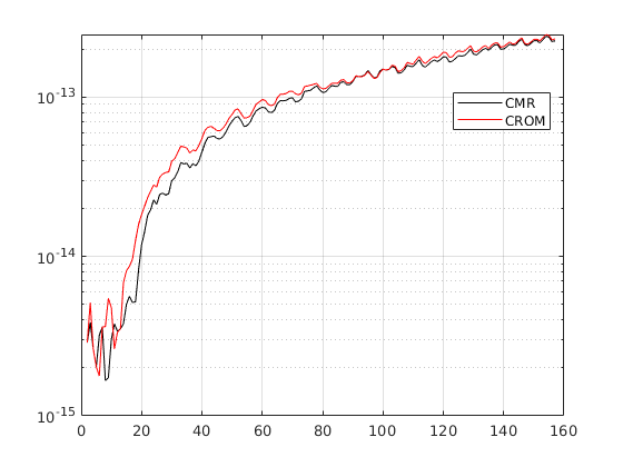
Refer to caption
Figure 4.6. Numerical simulation relative errors ‖ω^t−ω(t)‖∞/‖ω(t)‖∞\|\hat{\omega}_{t}-\omega^{(t)}\|_{\infty}/\|\omega^{(t)}\|_{\infty} with I​n​dε​(Σω)=(140,17)Ind_{\varepsilon}(\Sigma_{\omega})=(140,17) for ε=𝒪⁡(1×10⁻⁷)\varepsilon=\mathcal{O}(1\times 10^{-7})

4.2.3. UAC for predictive numerical simulation of time evolution of pure states in quantum systems

Let us start by considering the Schrödinger equation for a quantum harmonic oscillator model that can be written in the form

(4.8) i​∂ψ∂t−H​ψ=0i\frac{\partial\psi}{\partial t}-H\psi=0

where the Hamiltonian HH is determined by the expression.

H=−12​∂2∂x2+12​x2H=-\frac{1}{2}\frac{\partial^{2}}{\partial x^{2}}+\frac{1}{2}x^{2}

For some suitable boundary and initial conditions for the wave function ψ\psi on the boundary ∂Ω\partial\Omega of Ω=[−1,1]\Omega=[-1,1]. Let us consider a pure state ψ⁡(x,t)=ei​λ​t​Ψ​(x)\psi(x,t)=e^{i\lambda t}\Psi(x). We will have that Ψ\Psi satisfies the equation.

(4.9) H​Ψ=i​λ​ΨH\Psi=i\lambda\Psi

We can apply algorithm 1 to compute a UAC for the numerical simulation of the time evolution of pure states that satisfy (4.8) and (4.9).

In order to simulate the signal data corresponding to a quantum system determined by (4.8) and (4.9). We start by solving the difference equations (4.10) corresponding to (4.8) and (4.9), using finite difference methods implemented in MatLab.

(𝟏N+i​ht2​Hh)​ψ(n+1)\displaystyle\left(\mathbf{1}_{N}+\frac{ih_{t}}{2}H_{h}\right)\psi^{(n+1)} =(𝟏N−i​ht2​Hh)​ψ(n),\displaystyle=\left(\mathbf{1}_{N}-\frac{ih_{t}}{2}H_{h}\right)\psi^{(n)},
(4.10) Hh​ψ(1)\displaystyle H_{h}\psi^{(1)} =i​λ​ψ(1)\displaystyle=i\lambda\psi^{(1)}

Then, we computed the approximate solvents ψ(n)\psi^{(n)} of (4.8) determined by (4.10), that can be used as "noisy" input data for the UAC algorithm 2 implemented in MatLab as well, in order to compute predictive numerical simulations for the wave functions’ sampled data Σψ={ψ(k)}k=1N\Sigma_{\psi}=\{\psi^{(k)}\}_{k=1}^{N}, that are determined by the two UAC decompositions obtained by applying algorithm 4 and algorithm 5, that have the form.

(4.11) Σ^ψ:{ψ^t+1=𝒯^t​ψ^1ψ^1=ψ(1)‖ψ(t)−ψ^t‖≤ε,t≥1\hat{\Sigma}_{\psi}:\left\{\begin{array}[]{l}\hat{\psi}_{t+1}=\hat{\mathcal{T}}_{t}\hat{\psi}_{1}\\ \hat{\psi}_{1}=\psi^{(1)}\\ \|{\psi}^{(t)}-\hat{\psi}_{t}\|\leq\varepsilon\end{array}\right.,t\geq 1

The graphical outputs corresponding to the predictive numerical simulation for OPENψ^t+1)\hat{\psi}_{t+1}) computed with the UAC algorithm based on the 𝕌​ℂ​ℝ​𝕆​𝕄\mathbb{UCROM} method, are presented in figure 4.7.

Refer to caption
Figure 4.7. Predictive numerical simulation computed using UAC for Re⁡(ψ(t))\mathrm{Re}(\psi^{(t)}) (top) and Im⁡(ψ(t))\mathrm{Im}(\psi^{(t)}) (bottom), with I​n​dε​(Σψ)=(0,136)Ind_{\varepsilon}(\Sigma_{\psi})=(0,136) for ε=𝒪⁡(1×10⁻³)\varepsilon=\mathcal{O}(1\times 10^{-3})

The pseudospectra of the connecting matrices 𝒯1^\hat{\mathcal{T}_{1}} in (4.11) for CROM and UCROM methods are presented in figure 4.8.

Refer to caption
Refer to caption
Figure 4.8. Pseudospectra σε​(𝒯^1)\sigma_{\varepsilon}(\hat{\mathcal{T}}_{1}) of the low rank representations of the connecting matrices 𝒯^1\hat{\mathcal{T}}_{1}: CROM method (left) and UCROM method (right) with I​n​dε​(Σψ)=(0,136)Ind_{\varepsilon}(\Sigma_{\psi})=(0,136) for ε=𝒪⁡(1×10⁻³)\varepsilon=\mathcal{O}(1\times 10^{-3}).

The relative errors with respect to ∥⋅∥∞\|\cdot\|_{\infty} for the CROM and the UCROM method are presented in 4.9.

Refer to caption
Figure 4.9. Numerical simulation relative errors ‖ψ^t−ψ(t)‖∞/‖ψ(t)‖∞\|\hat{\psi}_{t}-\psi^{(t)}\|_{\infty}/\|\psi^{(t)}\|_{\infty} with I​n​dε​(Σψ)=(0,136)Ind_{\varepsilon}(\Sigma_{\psi})=(0,136) for ε=𝒪⁡(1×10⁻³)\varepsilon=\mathcal{O}(1\times 10^{-3})

5. Conclusion and Future Directions

The results in §3 allow one to derive computational methods like the ones described in §4.1, for finite state approximation and predictive simulation of the dynamical behavior of a data-driven system determined by some data sampled from a set of valid/feasible states.

Some applications of the algorithms in §4.1 to data-based schemes that can be used for model predictive control of industrial processes, will be presented in future communications.

The connections of the results in §3 to the solution of problems related to controllability and realizability of finite-state systems in classical and quantum information and automata theory, in the sense of [2, 1, 9, 3], will be further explored.

Further applications of cyclic finite-state approximation schemes to industrial automation and Building Information Modeling technologies, will be the subject of future communications.

Acknowledgment

The structure preserving matrix computations needed to implement the algorithms in §4.1, were performed with Matlab R2018b Update 5 (9.5.0.1178774) 64-bit (glnxa64) and FreeFEM 4.200001 64bits at the Scientific Computing Innovation Center (CICC-UNAH) of the National Autonomous University of Honduras.

I would like to thank the Organizing Committees of GPOTS 2019 and COSy 2019 at Texas A&M University and University of Regina, respectively, for the support received. Much of the research reported in this document was carried out while I was participating in the events.

I am grateful with Terry Loring, Marc Rieffel, Kenneth Davidson, Masoud Khalkhali, Jorge Destephen, Alexandru Chirvasitu, Douglas Farenick, Leonel Obando, Mario Molina, William Fúnez, Aner Godoy and Norman Sabillón for several interesting questions and comments, that have been very helpful for the preparation of this document.

References

  • [1] A. M. Bloch, R. W. Brockett, and C. Rangan. Finite controllability of infinite-dimensional quantum systems. IEEE Transactions on Automatic Control, 55(8):1797–1805, Aug 2010.
  • [2] R. Brockett and A. Willsky. Finite group homomorphic sequential system. IEEE Transactions on Automatic Control, 17(4):483–490, August 1972.
  • [3] R. W. Brockett. Reduced complexity control systems. IFAC Proceedings Volumes, 41(2):1 – 6, 2008. 17th IFAC World Congress.
  • [4] D. L. Elliott. Bilinear Control Systems Matrices in Action, volume 169 of Applied Mathematical Sciences. Springer, 2009.
  • [5] M. Farhood and G. E. Dullerud. Lmi tools for eventually periodic systems. Systems & Control Letters, 47(5):417 – 432, 2002.
  • [6] R. A. Horn. Topics in Matrix Analysis. Cambridge University Press, USA, 1986.
  • [7] J. L. Proctor, S. L. Brunton, and J. N. Kutz. Dynamic mode decomposition with control. SIAM J Appl. Dyn. Syst., 15(1):142–161, 2016.
  • [8] P. J. Schmid. Dynamic mode decomposition of numerical and experimental data. J. Fluid Mech., 656:5–28, 2010.
  • [9] D. C. Tarraf. An input-output construction of finite state ρ/μ\rho/\mu approximations for control design. IEEE Transactions on Automatic Control, 59(12):3164–3177, Dec 2014.
  • [10] L. Trefethen and M. Embree. Spectra and Pseudospectra: The behavior of nonnormal matrices and operators. Princeton University Press, 01 2005.
  • [11] F. Vides. On uniform connectivity of algebraic matrix sets. Banach J. Math. Anal., 13(4):918–943, 2019.
  • [12] F. Vides. Matlab functions for the computation of some universal algebraic controllers, 2020. https://github.com/FredyVides/UAC.