Self-consistent Semi-analytic Modeling of Feedback During Primordial Star Formation and Reionization
Abstract
We present a new semi-analytic model of the formation of the first stars. Our method takes dark matter halo merger trees (including 3-dimensional spatial information) from cosmological N-body simulations as input and applies analytic prescriptions to compute both the Population III (Pop III) and metal-enriched star formation histories. We have developed a novel method to accurately compute the major feedback processes affecting Pop III star formation: H2 photodissociation from Lyman-Werner (LW) radiation, suppression of star formation due to inhomogeneous reionization, and metal enrichment via supernovae winds. Our method utilizes a grid-based approach relying on fast Fourier transforms (FFTs) to rapidly track the LW intensity, ionization fraction, and metallicity in 3-dimensions throughout the simulation box. We present simulations for a wide range of astrophysical model parameters from . Initially long-range LW feedback and local metal enrichment and reionization feedback dominate. However, for we find that the star formation rate density (SFRD) of Pop III stars is impacted by the combination of external metal enrichment (metals from one halo polluting other pristine halos) and inhomogeneous reionization. We find that the interplay of these processes is particularly important for the Pop III SFRD at . Reionization feedback delays star formation long enough for metal bubbles to reach halos that would otherwise form Pop III stars. Including these effects can lead to more than an order of magnitude decrease in the Pop III SFRD at compared to LW feedback alone.
Keywords:
stars: Population III – galaxies: high-redshift – cosmology: theoryI Introduction
Simulations based on the standard model of cosmology predict that the first Pop III stars formed within Myr after the Big Bang in small dark matter “minihalos” (Greif 2015, for a recent review see). Currently, there are no definitive observations of Pop III stars, but a variety of upcoming facilities are positioned to improve constraints and may lead to unambiguous observational evidence. Radio telescopes targeting the cosmological 21cm signal (Furlanetto et al. 2006; Pritchard & Loeb 2012), both the global sky-averaged spectrum (Bowman et al. 2018; Price et al. 2018, e.g., EDGES and LEDA,) and spatial fluctuations (DeBoer et al. 2017; Koopmans et al. 2015, e.g., HERA and SKA,), are able to study the first stars through their impact on the intergalactic medium (IGM) (Visbal et al. 2012; Fialkov et al. 2013; Cohen et al. 2017; Bowman et al. 2018, e.g.,). Observations of extremely metal poor stars in the local Universe, which will be rapidly identified with the next generation of 30-meter class telescopes, can constrain the properties of the first stars (Hartwig et al. 2015; Hartwig et al. 2018b; Magg et al. 2018, e.g.,). Pop III stars in the mass range of may end their lives as extremely bright pair instability supernovae, which can potentially be detected with the James Webb Space Telescope (JWST) (Whalen et al. 2013; Hartwig et al. 2018a). Additionally, helium recombination line-intensity mapping may be able to constrain the global star formation history of Pop III stars (Visbal et al. 2015a) and it is possible to detect the impact of the first stars on the ionization fraction of the high-redshift IGM with cosmic microwave background (CMB) measurements (Kaplinghat et al. 2003; Haiman & Holder 2003; Ahn et al. 2012; Visbal et al. 2015b; Miranda et al. 2017, e.g.,).
In order to make accurate predictions for these observational probes, it is necessary to model the abundance of Pop III stars as a function of time. This requires accounting for a number of important feedback processes including metal enrichment from supernovae winds, suppression of star formation from hydrogen ionizing radiation, and LW photodissociating radiation, which suppresses or delays Pop III star formation in small dark matter halos (Haiman et al. 1997; Machacek et al. 2001; O’Shea & Norman 2008). A key challenge is that these processes operate over a vast range of distance scales. For example, metal enrichment due to Pop III supernovae explosions acts within individual dark matter halos or nearby regions of the IGM ( comoving kpc). On the other hand, LW feedback is due to the total LW flux from stars within Mpc of any potential star-forming halo (Ahn et al. 2009). We note that X-ray feedback due to gas accretion onto black hole remnants of primordial stars may operate on even larger scales (Madau et al. 2004; Ricotti & Ostriker 2004; Ricotti et al. 2005; Tanaka et al. 2012), however we do not include black hole modeling and X-ray feedback in this paper. We defer its treatment for future work.
Several different theoretical approaches have been utilized to make predictions for the abundance of Pop III stars. The most detailed calculations are hydrodynamical cosmological simulations including star formation, radiative feedback, and metal enrichment via supernovae winds (Wise et al. 2012a; Wise et al. 2012b; Wise et al. 2014; O’Shea et al. 2015; Xu et al. 2016, e.g.,). Simulations permit the most accurate treatment of the relevant physical processes, but are computationally expensive (O’Shea et al. 2015; Xu et al. 2016, e.g., tens of millions of CPU-hours for the Renaissance simulations). Despite their sophistication, numerical simulations still require subgrid physics which is put in by hand. This includes the Pop III IMF, the metal-enriched IMF, and the critical metallicity for the Pop III/Pop II transition. The numerical demands restrict hydrodynamical cosmological simulations to relatively small ( Mpc) simulation boxes (or zoom-ins) and limit the number of runs which can be performed to explore the parameter space of sub-grid physics.
The other extreme, in terms of theoretical approaches, is to use analytic calculations which can rapidly model large effective volumes and the uncertain parameter space of the high-redshift Universe. The simplest treatments involve estimating a minimum mass of dark matter halo that hosts Pop III stars and integrating over the halo mass function (Choudhury & Ferrara 2005; Mesinger et al. 2005; Wyithe & Cen 2007; Trenti & Stiavelli 2009; Haiman & Bryan 2006; Visbal et al. 2015b, e.g.,). These calculations are numerically inexpensive, but typically lack 3-dimensional spatial information and halo merger histories which are important for feedback and observational predictions. Additionally, halo merger histories can be modeled rapidly with Monte Carlo methods (Magg et al. 2016, as in), but this approach still lacks 3-dimensional spatial information. We note that in some instances, 3-dimensional clustering has been modeled analytically (Scannapieco & Barkana 2002; Scannapieco et al. 2003; Kramer et al. 2006). In Scannapieco et al. 2003, an analytic treatment of clustering was utilized to determine the abundance of Pop III stars as a function of cosmic time, including the impact of metal pollution due to supernovae winds. However, in contrast to the models presented here, they do not take into account the impact of cosmic reionization and the baryon-dark matter streaming velocities (Tseliakhovich & Hirata 2010). Kramer et al. 2006 have incorporated photo-ionization feedback into a toy-model that approximates source clustering, but only in the radial direction away from sources, whereas here we capture the full three-dimensional clustered distribution of the ionizing sources.
In this paper, we focus on a hybrid method between the numerical and analytic approaches just described. This “semi-analytic” method utilizes dark matter-only cosmological N-body simulations to determine the spatial and merger properties of dark matter halos. Analytic prescriptions are then applied to the dark matter merger trees to track both Pop III and metal-enriched star formation. Semi-analytic models allow much faster computations compared to hydrodynamical simulations (each run of our model presented below takes roughly 24 CPU-hours) and can incorporate more detailed physics than purely analytic methods. The computational efficiency of our method makes rapid parameter space exploration possible. This method can also be used to predict the scatter in observables due to random changes in initial conditions (cosmic variance).
A number of previous works have utilized semi-analytic simulations to study the first stars and galaxies (Trenti et al. 2009; Agarwal et al. 2012; Crosby et al. 2013; Valiante et al. 2016; Mebane et al. 2018; Visbal et al. 2018; Mebane et al. 2019, e.g.,). Some of these works have focused on predictions for Pop III or second generation stars which could be found in the Milky Way at (Griffen et al. 2016; Ishiyama et al. 2016; de Bennassuti et al. 2017; Graziani et al. 2017; Magg et al. 2018, e.g.,). There have also been efforts to model galaxies during the epoch of reionization without following Pop III stars or minihalos (Poole et al. 2016; Mutch et al. 2016; Yung et al. 2019a; Yung et al. 2019b). We also note that semi-analytic methods have been very useful in the context of more evolved galaxies at low redshift (Baugh 2006; Lu et al. 2014, e.g.,).
In addition to N-body simulations or Monte Carlo merger trees, semi-analytic models can be created using dark matter halos simulated with a code such as pinocchio (Monaco et al. 2002), which utilizes Lagrangian Perturbation Theory (LPT) to rapidly model the formation and properties of halos in cosmological volumes. This has been applied to the problem of Pop III star formation in Banik et al. 2019 (though they use a much simpler model of feedback processes than the present work). The LPT and N-body methods are complementary in the sense that LPT can generate larger cosmological volumes at low computational expense, but N-body simulations can more accurately capture the small-scale properties of halos (e.g., clustering on non-linear scales). In future work, a detailed side-by-side comparison would be helpful to determine the exact limitations of the LPT approach in the context of the first stars.
The main new feature of our model presented below is a grid-based approach to calculate the major feedback processes for Pop III star formation: LW feedback, suppression of star formation due to photoheating from reionization, and metal enrichment due to supernovae winds. Our grid-based method utilizes FFTs to rapidly compute the 3-dimensional LW intensity, ionization fraction, and metallicity throughout our simulation box. We note that these models are also the first of their type to include a treatment of the baryon-dark matter velocities (Tseliakhovich & Hirata 2010), which suppress star formation in small dark matter halos in high-velocity regions (Fialkov et al. 2012).
We utilize this method to compute the Pop III and metal-enriched star formation histories across cosmic time for a range of the uncertain model parameters describing star formation and feedback. Detailed results are presented below. We find that spatial clustering of feedback effects begins to be important at , when a significant fraction of the IGM is ionized. We also find that at high redshifts, star formation is strongly impacted by the baryon-dark matter streaming velocity. Another important conclusion is that the timing of the cosmic transition between Pop III and metal-enriched star formation is likely set by the delay between initial metal-free star formation and second generation star formation due to supernovae explosions of Pop III stars.
This paper is structured as follows. In Section 2, we describe the cosmological simulations utilized by our model. We explain the details of our model in Section 3 and present results for the Pop III and metal-enriched cosmic star formation histories for a range of model parameters in Section 4. Finally, we discuss our results and main conclusions in Section 5. Throughout, we assume a cosmology with parameters consistent with Planck Collaboration XVI 2014: , , , , , and .
II N-Body Simulations
We utilize the publicly available code gadget2 (Springel et al. 2001) to produce the cosmological N-body simulations required for our semi-analytic model. To improve the statistics of our results, we ran 10 simulations, each with a different random seed for the initial conditions. All of these simulations have a 3 Mpc box length and particles. This corresponds to a particle mass of . Initial conditions were generated with 2LPTIC (Crocce et al. 2006) and created at . For each run, snapshots were saved from to , spaced in cosmic time by , where is the Hubble time at the preceding snapshot. This time spacing corresponds to of the dynamical time of a halo at its virial radius, which we find is sufficient for convergence in our semi-analytic model. Halo catalogs and merger trees were computed using the publicly available codes rockstar (Behroozi et al. 2013a) and consistent trees (Behroozi et al. 2013b). We emphasize that the selected mass resolution is sufficient for our semi-analytic models. As discussed below (see Figure 4), the first Pop III stars in our model form in dark matter halos. These are resolved with dark matter particles in our N-body simulations. rockstar has been shown to accurately determine halo properties for halos with particles (Behroozi et al. 2013a; Knebe et al. 2011). Previous work has also shown that substructure in dark matter halos can be tracked for subhalos with particles (Onions et al. 2012). We do not attempt to track substructure in our model, leading to a less stringent requirement. Thus, we regard our 250 particle resolution as a relatively conservative choice. We also note that the simulated halo mass functions agree very well with the analytic mass function of Sheth & Tormen 1999 (Visbal et al. 2018, see Figure 1 in).
| Parameter | Description | Fiducial Value | Range |
| Pop III star formation efficiency | 0.001 | ||
| Metal-enriched star formation efficiency | 0.05 | – | |
| LW/Ionizing photons per baryon of metal-enriched stars | 4000 | – | |
| LW/Ionizing photons per baryon of Pop III stars | 65000 | – | |
| Delay in subsequent star formation due to Pop III SNe | yr | ||
| Critical metallicity for externally metal-enriched halos | |||
| Critical mass for externally metal-enriched halos | |||
| Ionization feedback mass | |||
| Ionizing escape fraction in metal-enriched halos (Section 3.3) | 0.1 | ||
| Ionizing escape fraction in Pop III halos (Section 3.3) | 0.5 | ||
| Streaming velocity at recombination | () | ||
| Metal bubble size scaling factor (Section 3.4) | 1 | ||
| Minimum halo mass for Pop III star formation | see Eqns. 1-3 | – |
III Semi-analytic Model
Broadly speaking, our semi-analytic model takes as input the merger history and 3-dimensional spatial information of dark matter halos from an N-body simulation. It then utilizes analytical prescriptions to determine where, when, and how much Pop III and metal-enriched star formation occur. These prescriptions include major feedback processes relevant for Pop III star formation: LW feedback, reionization of the IGM, and metal enrichment from supernovae winds. This physics is characterized by a number of model parameters which are listed with their fiducial values in Table 1.
The most important novel feature of the model is a grid-based method for computing feedback processes which depend on the 3-dimensional positions and clustering of dark matter halos. As described in the following subsections, this method utilizes FFTs to rapidly compute the local values of the LW intensity as well as the metallicity and neutral fraction of the IGM throughout the simulation box. The new method allows us, for the first time, to rapidly compute HII regions due to ionizing photons from Pop III stars and metal-enriched galaxies including the impact of multiple sources inside ionization bubbles (Furlanetto et al. 2004, this was inspired by work on larger distance scales, such as). This is not properly accounted for in simpler ‘shell’ models that have been employed in previous semi-analytic simulations tracking Pop III star formation (Magg et al. 2018; Visbal et al. 2018, e.g.,). A shell approach which computes an ionized bubble radius for each source separately and does not take into account how nearby ionizing sources both ionize some of the same portion of the IGM, underestimates the total ionized volume around these clustered sources.
III.1 Star formation
Dark matter halos throughout the simulation box are assigned both Pop III and metal-enriched star formation. Pop III star formation occurs when a pristine halo (i.e. no external/internal metal enrichment as described below) first reaches the minimum mass where gas can cool and form stars. For metal-free minihalos, this cooling is due to molecular hydrogen transitions. Hydrogen molecules are photo-dissociated by LW radiation, which can suppress Pop III star formation in smaller minihalos (Haiman et al. 1997; Machacek et al. 2001; Wise & Abel 2007; O’Shea & Norman 2008; Wolcott-Green et al. 2011; Visbal et al. 2014). The baryon-dark matter streaming velocity (Tseliakhovich & Hirata 2010) can also suppress star formation in small minihalos (Fialkov et al. 2012). Considering both of these effects, we assume that for halos which are not in an ionized region of the IGM, the minimum mass for Pop III star formation is
| (1) |
where
| (2) |
is the minimum mass for molecular cooling in minihalos (Fialkov et al. 2013) and is the atomic cooling threshold found in hydrodynamical cosmological simulations (Fernandez et al. 2014, with the precise value taken from the simulations of). The local value of the LW background, , is given in units of . Here is the cooling mass for a minihalo without LW radiation as a function of redshift and the local baryon-dark matter streaming velocity, . Note that the value of the streaming velocity evolves as and has a typical value of 30 (the root-mean-square value which we denote as ) at recombination. We compute from the following fitting function calibrated to hydrodynamical simulations by Fialkov et al. 2012,
| (3) |
In this formula, is the circular velocity corresponding to the viral mass (Barkana & Loeb 2001, as defined in) and the fit parameters are and (Greif et al. 2011; Stacy et al. 2011, which are determined from the simulations of). On scales of the streaming velocity is roughly constant, so for any particular run, we assume one value of the streaming velocity. We note that because our N-body simulations are dark matter only, we are not able to incorporate the reduction in the halo mass function due to high (Tseliakhovich & Hirata 2010). However, this is a modest effect (Naoz et al. 2012, e.g., 20 percent reduction of halos at for ,) and should be secondary compared to the delay in molecular cooling as described in Fialkov et al. 2013. Future work could use hydrodynamical cosmological simulations to compute merger trees with the streaming velocity included. We note that the fit in Eq. 2 is based on a relatively small number of hydrodynamical simulations. Future work exploring a larger range of redshifts and combining streaming velocities and LW feedback will be important to accurately tune models like those presented in this paper.
When a pristine halo reaches , we assume that Pop III stars are formed with an efficiency (i.e. a total mass of Pop III stars are formed). We also assume that there is then a delay, , due to the lifetime of the stars and recovery from SN explosions before metal-enriched star formation can occur. The recovery time is needed for gas to resettle in a halo’s gravitational potential well after being disrupted by SNae. We assume a fiducial value of , which represents recovery from a core collapse SN (Jeon et al. 2014) in a minihalo. The delay in efficient metal mixing could take longer in more massive dark matter halos. The impact of increasing is discussed in detail below (which is significant for the timing of the cosmic transition from Pop III to metal-enriched star formation). Once a time greater than has passed in a halo (starting from the earliest Pop III episode if there are multiple Pop III progenitors), metal-enriched star formation begins. We assume that across each time step in our simulations (which are the same as the N-body snapshots, set to of the dynamical time of a dark matter halo at the virial radius as described in Section 2), the metal-enriched star formation rate is
| (4) |
where is the mass accreted from halos without stars or in smooth accretion (including halos below the resolution of the simulation) and is the time between N-body simulation snapshots. Thus, a minihalo which hosts Pop III star formation must accrete additional material or merge with other pristine minihalos before it can form a significant amount of metal-enriched stars in our model. We find that this typically happens over our assumed values of . In our fiducial model, we have adopted a metal enriched star formation efficiency of , which we take from Visbal et al. 2015b. This value was determined using abundance matching and the observed UV luminosity function of galaxies at from Bouwens et al. 2015. We note that the Pop III star formation efficiency is not tightly constrained by simulations. We have adopted a fiducial value of , which corresponds to of stars in a minihalo and is compatible with the CMB optical depth due to electron scattering with our fiducial set of model parameters (Visbal et al. 2015b).
In addition to internal enrichment (i.e. star formation and enrichment in the same halo as just described), we also include external enrichment (supernovae winds from one halo enriching another separate halo). As discussed below, we use our grid-based approach to track the metallicity of the IGM and if a halo with mass above is in a region with metallicity above , we assume that metal-enriched star formation proceeds according to Eq. 4. We assume a fiducial value of , but note that this is a highly uncertain quantity. For , we assume a fiducial value of . There have been a number of previous studies attempting to determine this quantity (Bromm & Loeb 2003; Omukai et al. 2005; Smith & Sigurdsson 2007; Smith et al. 2009, e.g.,). These works tend to find a critical value near our fiducial choice, but it could be significantly lower () if dust cooling is important, rather than just C and O (Omukai et al. 2005).
We also include the impact of reionization of the IGM. The neutral fraction of the simulation box is tracked with the grid-based method as described below (assumed to be 0 or 1 in each resolution element of our grid). Gas heating due to reionization has been shown to impede star formation in smaller dark matter halos (Shapiro et al. 1994; Thoul & Weinberg 1996; Gnedin & Hui 1998; Gnedin 2000; Dijkstra et al. 2004; Hoeft et al. 2006; Okamoto et al. 2008; Sobacchi & Mesinger 2013; Noh & McQuinn 2014, e.g.,). In our model, if a halo without prior star formation is in an ionized region, the minimum mass is raised (in the fiducial model) to (Dijkstra et al. 2004, consistent with). For a halo in an ionized region which already has star formation, the metal-enriched star formation is reduced by a factor of , where is the time since reionization for the first progenitor halo which was reionized. This factor’s characteristic timescale is equal to the dynamical time at the virial radius of a recently formed dark matter halo, . We include this timescale to account for the fact that star formation may not be instantaneously quenched when the IGM surrounding a galaxy is ionized. Dense gas in the halo which is already flowing towards the center may not be strongly impacted even if lower density gas in the surrounding IGM (outside of the halo) is ionized.
Our LW and ionizing feedback prescriptions, described in detail below, depend on the amount of LW and ionizing radiation produced by stars. We assume that the number of hydrogen ionizing photons produced per baryon incorporated into stars is and , for metal-enriched and Pop III stars, respectively. The metal enriched value corresponds to a Salpeter IMF from 0.1 to 100 and metallicity (Samui et al. 2007, see table 1 in). The Pop III value is expected for a star over its lifetime (Schaerer 2002). For simplicity, we assume one LW photon is created for each ionizing photon. This assumption may underestimate the LW flux by a factor of a few for metal-enriched galaxies. Given the relatively large uncertainties in a number of astrophysical parameters (e.g., the star formation efficiencies), we leave a more detailed treatment for future work. We also note that we have assumed a LW escape fraction of unity throughout this paper. We do not expect this to have a strong effect on our results, but note that there could be an impact for cases with very low star formation efficiency (Schauer et al. 2015).
Finally, we note that we do not include subhalos in our model. The only halos considered are distinct halos which are not substructure of more massive halos. We also note that we do not allow “splash-back” halos (i.e. those subhalos which enter and then leave a larger halo) to contribute to star formation. This is to prevent double-counting star formation. A splash-back halo contributes to star formation when it first enters a halo, and we do not include more star formation if it exits and re-enters.
III.2 LW Feedback
We calculate the LW flux incident on a minihalo as , where is the local flux from nearby individual sources and is the mean LW background on large scales generated by sources outside of the simulation box. The uniform background from sources beyond the simulation box is given by
| (5) |
where is the mean LW emissivity in our box as a function of redshift, is the Hubble time, and the attenuation of LW flux observed at redshift from sources at redshift due to LW photons being redshifted into Lyman series resonance lines and absorbed (Haiman et al. 1997). We approximate this attenuation with Eq. 22 in Ahn et al. 2009. The limit of integration, , corresponds to the redshift of an object at a distance from an observer at , due to the finite light travel time. Thus, for each halo, the LW contribution from distances greater than is given by and by for distances smaller than . When computing the integral in Eq. 5, we smooth over a redshift range corresponding to a change in cosmic time of 10 Myr. This is meant to reduce rapid fluctuations, which are not expected in the background component (which has contributions from Mpc scales). Additionally, for very high redshift, when there are few sources, we set the large-scale background by hand to mimic the contribution from stars formed outside of the simulation box. We find that setting at maps smoothly onto the background flux calculated with Eq. 5 at lower redshifts in our fiducial model. This ad hoc procedure only impacts the very highest redshift in our simulations. As discussed in Section 5, due to the small size of our box we cannot hope to accurately determine the global LW background. In future work, we intend to combine the semi-analytic models described in this paper with larger-scale models ( Mpc) to simultaneously capture large-scale and small-scale astrophysical effects.
When computing the local LW contribution, , we adopt a grid-based method. We break our simulation box into a cubic grid with cells. We find that the results have converged for this resolution, reducing the resolution to changes the Pop III and metal-enriched SFRD by percent or less. This is expected since the grid has a spatial resolution of kpc (comoving), which is approximately equal to the virial radius of an atomic cooling halo at . For a pristine halo in cell , the LW intensity coming from all other cells is well approximated as
| (6) |
where is the LW energy currently emitted from stars in cell , per time, per frequency, divided by and is the position of the ’th cell. We note that using the convolution theorem, this can be rapidly computed using FFTs. We compute Eq. 6 using
| (7) |
where signifies convolution and and denote the discrete Fourier and inverse Fourier transforms, respectively. We compute these with FFTs on our grid, utilizing periodic boundary conditions to determine for each cell and setting the contribution from halos to their own cell (i.e., ) to zero. We then add the contribution from halos within the same cell using the exact distance to ensure that close halo pairs are treated accurately. In our fiducial model, there are very few minihalos with star-forming halos in the same cell (there are sources spread among 2563 cells at ). We find that this approximate method quickly computes essentially the same LW fluxes as would be obtained by a brute force calculation computing the distance squared between all relevant pairs of halos (for most halos the difference in the computed local LW intensity between the two methods is less than 10 percent).
III.3 IGM Ionization State
As discussed above, regions of the IGM that have been reionized will be photoheated, which can suppress star formation in small dark matter halos ( in our model parameterization). In order to compute the ionization fraction throughout our box, we utilize a grid-based method inspired by larger-scale semi-numerical approaches used in the past (Furlanetto et al. 2004; Zahn et al. 2005; Mesinger & Furlanetto 2007; Mesinger et al. 2011, e.g.,). At each redshift, we begin with a resolution cubic grid , where each cell contains the total number density of ionized photons previously produced in all the dark matter halos within that cell that have escaped into the IGM. This is given by , where and are the total masses of metal-enriched and Pop III stars ever formed in cell i and is the comoving density of each cell. Here and denote the escape fraction of hydrogen ionizing photons from halos hosting Pop III and metal-enriched stars, respectively. We smooth on a range of scales, corresponding to different ionized bubble sizes, . After smoothing on a given bubble size, we identify cells which are the center of -sized spheres which have a total number of ionizing photons per bubble volume greater than a threshold . These cells are set to be the centers of ionized bubbles of radius . If one follows this procedure for an isolated source of ionizing radiation, selecting (where is the cosmic mean comoving density of hydrogen atoms) gives an ionized bubble around the source with a size that exactly corresponds to the number of ionized photons produced by the source (ignoring recombinations). However, if there are a number of sources which are distributed over a spatially extended region that contribute to the same ionized bubble, one must select a higher value of to correctly recover the bubble size. Thus, the exact value of which should be used depends on the clustering of the sources within the box. We find that using leads the total ionization fraction to be within of the total number of escaped ionizing photons in the box divided by the total number of hydrogen atoms in the box.
We find that our model converges for 30 logarithmically-spaced bubble radii ranging from one cell to half the length of the box. The smoothing mentioned above is rapidly computed with FFTs by applying the convolution theorem to and a spherical top-hat window function centered around the origin. Note that this method does not include recombinations. In Visbal et al. 2018, we found that recombinations did not have a significant impact on our semi-analytic results for the redshifts explored (). This is due to the rapid increase in star formation as a function of time. By the time a region could recombine, a much larger number of ionizing photons have been produced in the same region. At later times adding recombinations could potentially slow the growth of bubbles in our simulations, however given the other uncertainties in the modeling (e.g., the time evolution and halo mass dependance of the escape fractions of ionized photons), we defer a detailed treatment to future work.
III.4 IGM Metallicity
Our semi-analytic model permits pristine halos to be externally polluted by SN winds, leading to metal-enriched star formation. Thus, it is necessary to compute the metallicity of the IGM throughout the simulation box. To accomplish this, we assume that SN winds create spherical metal bubbles around halos which begin expanding 4 Myr after star formation begins (this delay is caused by the lifetime of massive stars). Following Trenti et al. 2009, we assume that the bubble velocity is given by until it reaches a comoving radius of . We include a free parameter , which we vary to determine the impact of different bubble sizes on our results. We find that the bubble radius given by this procedure (with ) is in rough agreement with the hydrodynamic cosmological simulations of Smith et al. 2015, which include radiative transfer and resolve the blast-wave of the SN explosion. To compute the total amount of metals in each bubble, we assume of heavy elements are produced per each (chosen as the Pop III stellar mass for simplicity) of Pop III stars (Nomoto et al. 2006) and of metals are produced for every of Pop II stars (Barkana & Loeb 2001, this is the approximate metal yield assuming that stars above lead to a supernova and of heavy metals are produced per supernova). We assume metals are spread uniformly throughout each bubble and the metallicity is summed where bubbles overlap.
Similar to our approach to LW and ionization feedback, we utilize a cubic grid of resolution elements, and calculate the metallicity in each cell according to the metal bubble properties just described. We rapidly compute this grid by going though the same range of bubble sizes used for reionization, which are described in the preceding subsection. For each bubble size we take a grid populated with the centers of bubbles in that radius bin and smooth using the convolution theorem and FFTs. In Figure 1, we show projections of the ionization fraction and metallicity of the IGM computed with the grid-based methods discussed.
III.5 Computational Cost
Next we discuss the computational cost and scaling of our implementation of the method just described. The FFT-based method has a more efficient scaling with the size of the simulation compared to a simple approach which directly computes distances between pairs of dark matter halos. For instance, the naive approach to computing the LW fluxes on potential-Pop III-forming halos requires computing the distances between pairs of halos. So for fixed mass resolution, the compute time for this approach scales with the volume of the simulation box as (metal enrichment or reionization have the same scaling). For our FFT-based method however, populating the grid with sources of LW/ionizing radiation or metal bubbles scales as and the compute time of FFTs scales as , where is the number of elements in the grid. Thus, for fixed resolution our FFT based approach scales as least as fast as . We note that the shell method used in Magg et al. 2018 also performs better than the simple case for both external metal enrichment and reionization. This is possible because one can ignore pairs of halos which are at significantly larger distances than the relevant bubble sizes.
We note that, due to our small box, this improved scaling was not particularly important in our fiducial model. It takes second to compute the distance between pairs of halos on one of the cores of the Flatiron Institute’s computer cluster “Rusty”. It takes roughly the same time to compute an FFT on the grid used (note that the grid resolution does not need to match the N-body simulation’s resolution). By the end of our simulation () in the fiducial parameterization, we have roughly sources and minihalos which must be checked for LW flux/metal enrichment (in each of our 10 realizations). For this small number of pairs, directly computing the distances is fast. However the improved scaling leads to a significant speedup in models where many halos are externally metal enriched, leading to many more sources. In the cases presented below where metal bubbles reach minihalos before ionizing radiation we find many more halos with star formation (on the order of sources by ). In this case, where pairs of distances must be determined, the FFT approach is roughly an order of magnitude faster. In either case, for the box sizes we have chosen, the compute times are relatively modest. Thus, the fact that the FFT method can more accurately capture inhomogeneous reionization compared to previous shell models is more important for the results presented below. However, we point out that if much larger boxes were used, the scaling improvement of our FFT method would be much more pronounced.


IV Results
We begin by exploring how the cosmic star formation history is affected by various feedback mechanisms. In Figure 2, we show the evolving SFRD when including/excluding different combinations of LW feedback, external metal enrichment via supernovae winds, and cosmic reionization (while otherwise keeping the fiducial parameters in Table 1). The qualitative effects of these mechanisms can be understood as follows. Compared to the LW only case, including external metal enrichment slightly increases the metal-enriched SFRD and reduces the Pop III SFRD due to small halos neighboring star-forming halos being externally enriched. When only including LW and reionization feedback, the metal-enriched SFRD is significantly reduced compared to LW alone. This is due to the quenching of star formation in small halos due to gas photoheating described in section 3.1. We note that this reionization feedback is mainly local at high redshift (), halos ionize their surrounding regions of the IGM leading to the subsequent quenching of star formation. Compared to LW alone, there is also a small increase in the Pop III SFRD at , which results from the decreased LW background intensity at this redshift. This ultimately leads to a lower Pop III SFRD at because more of the halos have already been metal-enriched at higher redshift.
When adding all three feedback processes, the metal-enriched star formation history does not change much from the LW and reionization case. This is because the metal bubbles do not extend as far as the ionization bubbles in our fiducial model (see Figure 1). Thus, small halos neighboring star formation which are enriched by metals are also ionized and do not form any stars. Combining reionization and metal enrichment reduces the Pop III SFRD even more than each alone at . In this case, the ionization and external metal enrichment are acting in tandem. The ionization feedback first reaches a pristine halo and delays its Pop III star formation. Metals spread through the IGM arrive before the halo has reached a sufficient mass to form stars.
We note that both the metal-enriched and Pop III SFRDs have a feature at . This is due to the LW background put in by hand and changing at as described above. Putting this in by hand was necessary due to the small size of our box, however in future work we plan to combine these models with techniques incorporating larger spatial scales to address this issue.
The Pop III and metal enriched SFRDs in Figure 2 can be compared to a number of previous works. Observationally, Finkelstein 2016 reports the total SFRD density from the integration of UV luminosity functions (LFs) down to (Madau & Dickinson 2014, see also). These observational values decline from at to at . This is very similar to our fiducial model with all feedback mechanisms included (metal-enriched SFRD of and at and , respectively). While currently there are no observations of the Pop III SFRD, we can compare our results to previous theoretical models. We find that in our fiducial model, the Pop III SFRD is quite similar to the “classical” Pop III model from the hydrodynamical cosmological simulations of Sarmento et al. 2019 that do not include their sub-grid prescription for inefficient mixing of metal pollutants. Our results agree mostly within a factor of a few for most redshifts between (see their Figure 1). We note that the agreement in metal enriched SFRD is not as close (significantly higher SFRD at in our model). A qualitatively closer match could be obtained by increasing our (as discussed below). We also note good agreement with the Pop III SFRD from the numerical simulations of Xu et al. 2013, matching to roughly a factor of a few over (see their Figure 2). In contrast to Sarmento et al. 2019, Xu et al. 2013 find higher metal-enriched SFRD than our fiducial model. When comparing to the analytic model of Scannapieco et al. 2003, compensating for a factor of 100 difference in star formation efficiency, we find a similar Pop III SFRD to their model with the lowest energy driving metal bubbles into the IGM. A precise comparison is challenging however, due to major differences in modeling feedback processes (e.g, the impact of reionization). Broadly speaking there is qualitative agreement between our results and a number of other simulations and semi-analytic models (Johnson et al. 2013; Pallottini et al. 2014; Jaacks et al. 2018; Magg et al. 2018, e.g., ), but there remain order of magnitude quantitative variations in the high-redshift Pop III and metal enriched SFRDs (Sarmento et al. 2019, see Figure 1 in). This is not surprising due to the uncertainty of the properties of the first stars and illustrates the importance of rapid semi-analytic models to efficiently survey the relevant model parameter space.

Next, we examine how the star formation history is impacted for parameter variations (mostly changing one parameter at a time) around our fiducial model (with all feedback mechanisms included). These results are shown in Figure 3, where a number of parameters are adjusted. As expected, the Pop III star formation efficiency, , is the most important parameter impacting the amount of Pop III stars formed over cosmic time. We note that many of the parameters (i.e. , , ) do not have a strong impact on the cosmic abundance of Pop III stars in our fiducial model. The main exceptions are that at high redshift (above ) a high-streaming velocity, , greatly reduces the abundance of Pop III stars. At lower redshift (), the abundance of Pop III stars depends on and . This is because either reducing or increasing increases the number of pristine halos which are externally metal-enriched (in the latter case because Pop III star formation is delayed allowing metals to arrive). We note that when varying within the fiducial model for the values indicated in Table 1, there are minimal changes to either the Pop III or metal-enriched SFRD.
In the fiducial model, metal-enriched star formation quickly dominates over Pop III. However, we point out that the global transition from Pop III to metal-enriched star formation seems to be strongly controlled by the delay between Pop III and metal-enriched star formation due to SN feedback, . Increasing this timescale by a factor of five drastically changes metal-enriched star formation at early times. This is partly due to our specific prescription for reionization feedback. Pop III star formation generally reionizes the surrounding region and if is increased, the star formation suppression factor due to photoheating () becomes much smaller by the time metal enriched star formation can occur.
Two parameters that warrant further discussion are the escape fractions of ionizing radiation, and . From Figure 3, we see that the total amount of star formation is not strongly impacted by varying this parameter by a factor of three. Since the ionized bubbles envelop the entire box by this result initially seems unexpected. However, closer inspection reveals that while the total abundance of Pop III stars does not change, the halos where they form does. Thus, in the case with a lower escape fraction more Pop III stars form in lower mass halos, but because there is less gas mass, a lower amount of Pop III stars forms in each of these halos. The reason the abundance is so similar is due to the shape of the halo mass function. Over the relevant redshift and mass range, . Thus, if the minimum halo mass for star formation increases by some factor, the reduction in the amount of halos forming Pop III stars is very closely compensated by the increased amount of star formation due to the larger halo masses. This can be seen in Figure 4, where we show masses and redshifts of halos hosting Pop III star formation in the fiducial model compared to reducing the ionizing escape fractions by a factor of 3. At the fiducial model has fewer Pop III-forming halos, but they have closely compensating higher masses leading to a very similar Pop III SFRD (see Figure 3).
We also show how the fraction of the simulation box which is ionized and metal-enriched evolves over time (see Figure 5). As mentioned above, in our models the ionization fraction is generally much larger than the fraction of the IGM which is significantly enriched by metals. Even though the simulation box is far too small to accurately characterize reionization, we see that the box is completely ionized at (Planck Collaboration et al. 2016, which is roughly consistent with observational constraints such as the optical depth from).
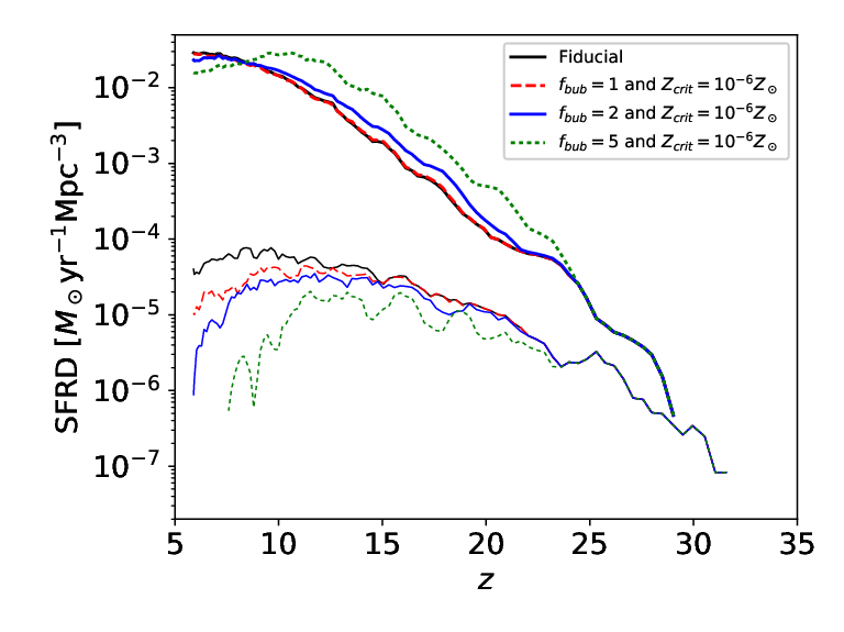
We have also considered cases varying and simultaneously. Increasing alone has very little impact on the Pop III SFRD because, for the fiducial , as the bubbles grow they dilute below the critical metallicity reducing the impact for external metal enrichment. This is not the case when simultaneously reducing the to the level corresponding to dust cooling and increasing . This is illustrated in Figure 6, where we see that, in extreme cases, external metal enrichment can quench Pop III star formation at earlier times or lead to an increase in early metal-enriched star formation due to external enrichment of minihalos. The latter effect only occurs if the metal bubbles expand faster than ionization bubbles to prevent the suppression of star formation discussed above.
In Figure 8 we include a comparison of our fiducial model to observations of the UV LF. We have converted SFR to UV magnitude via . This relation is based on the ratio of the dust-corrected SFRD to the luminosity density given in Bouwens et al. 2015. We note that aside from using a star formation efficiency that was set through abundance matching, we have made no detailed efforts to match to observations. It is encouraging to see agreement without more specific tuning. We do not dwell on this result as we have mainly focused on the physics of Pop III star formation in our modeling, but note that our simple model predicts a flattening for galaxies fainter than a rest-frame UV magnitude of .
We conclude this section by examining our choice of resolution in the grid-based feedback prescription for LW feedback, reionization, and external metal enrichment. In Figure 7, we plot the Pop III and metal enriched SFRDs for a model which differs from the fiducial case in two parameters ( and ) for various grid resolutions. External metal pollution is more extreme for these parameters compared to the fiducial model as discussed above. Thus, this parameterization provides a good check for convergence of external enrichment. Figure 7 shows good agreement for the resolutions plotted (, , and ) at most redshifts. However, we note that for the coarsest resolution, the metal-enriched star formation is not converged at . We see very good agreement between the and resolutions at all redshifts. The agreement is generally better than ten percent and justifies our choice of for the other results presented above.




V Discussion and Conclusions
In this paper, we have presented a new semi-analytic model of Pop III and metal-enriched star formation in the early Universe. This model takes in dark matter halo merger trees (including 3-dimensional clustering information) obtained from cosmological N-body simulations and applies analytic models to populate the halos with stars. The main new feature of these simulations is a grid-based approach to compute feedback from LW radiation, photoheating of gas due to inhomogeneous reionization, and metal bubbles in the IGM due to SN winds. These are the first semi-analytic models of Pop III star formation with both external metal enrichment and a prescription for reionization which takes into account inhomogeneous reionization properly including multiple ionizing sources contributing to the same HII region. We also note that the improved scaling of our grid-based technique ( compared to in the naive case) permits larger boxes in future work.
We applied our semi-analytic model to N-body simulations which resolve dark matter minihalos for a wide range of parameterizations spanning the parameters summarized in Table 1. We focus on results pertaining to Pop III stars, as our model is uniquely positioned to follow the important feedback processes for metal-free star formation. Overall, we find that adding a full 3-dimensional treatment of reionization and external metal enrichment can have a strong impact on the cosmic star formation history. Reionization feedback significantly reduces the metal-enriched SFRD at all redshifts. We note that at high redshift (), this reduction does not depend on the clustering of halos because it is caused by halos’ direct progenitors (and thus reducing the ionizing photon escape fraction does not affect the Pop III or metal-enriched SFRD in Figure 3). This is consistent with our results from Visbal et al. 2018. At , external metal enrichment and reionization work in tandem to reduce the Pop III SFRD by roughly an order of magnitude compared to LW feedback alone. Reionization delays star formation in pristine halos which are then enriched by metal bubbles before any Pop III stars can form.
Consistent with Magg et al. 2018, we both find that at late times there can be sustained Pop III star formation in regions of the IGM which have been reionized. This motivates additional hydrodynamical simulations of Pop III stars formed in these environments (Visbal et al. 2017; Kulkarni et al. 2019, for simulations in the case of high ionizing flux see).
When varying individual parameters around the fiducial model, we (unsurprisingly) find that (the fraction of pristine gas which forms stars in an episode of Pop III star formation) is the most important for setting the overall abundance of Pop III stars. Generally, we find that a significant (though subdominant) amount of Pop III star formation continues to . The behavior of the Pop III SFRD at low redshift depends strongly on the critical metallicity for metal-enriched star formation, and the mass below which ionization feedback operates, . For our fiducial model, it appears that the Pop III SFRD is not strongly decreasing with time at , however lowering or raising begins to quench Pop III star formation. While these parameters are the most important at lower redshifts, we point out that at high redshift the streaming velocity has a large impact. Increasing from to , substantially delays Pop III and metal-enriched star formation. Another important result is that at the Pop III SFRD does not change for most of our parameter variations (with the notable exceptions of and ). This is largely because the fraction of the box which is ionized and/or metal-enriched is quite low at early times (see Figure 5). We also point out that while increasing from our fiducial model did not have a strong affect on the Pop III SFRD, it did dramatically change the metal-enriched SFRD and sets a characteristic redshift where there is a transition from the dominance of Pop III to metal-enriched star formation.
Due to the importance of external metal enrichment at , we also explore simultaneously varying and . For a critical metallicity corresponding to dust cooling, , we find that increasing the size of the metal bubbles can greatly reduce the Pop III SFRD at . Increasing , but keeping does not have a strong impact on the Pop III SFRD. This is because the metals get spread out over larger bubbles leading the metallicities to drop below the critical value.
Several caveats must be kept in mind when interpreting our results. A shortcoming of the model is that the simulation boxes used are 3 Mpc across, while the horizon for LW photons is much larger ( Mpc). Thus, while the LW background intensity is computed self-consistently, it may not be accurate due to missing sources in rare over-dense regions which would be found in much larger simulation boxes. Future work combining smaller-scale models like those presented here with semi-numerical simulations such as those from Visbal et al. 2012; Fialkov et al. 2013 will be required to make accurate predictions of the overall abundance of Pop III stars (see also Ahn et al. 2012, for a subgrid prescription of minihalos in cosmic reionization). We also note that our star formation efficiencies ( and ) are taken as constants throughout. In reality, these quantities may have both redshift and halo mass dependences which needs to be taken into account. Future work making more detailed direct comparisons with numerical simulations will be required to determine the most accurate parameterization of the star formation efficiencies. When varying parameters, we have generally changed one at a time with respect to the fiducial model. Simultaneously altering multiple parameters could lead to interesting new qualitative behaviors (as we saw for varying and simultaneously), which we defer to future work. We also note that we have assumed very efficient mixing of metals in the IGM and in star-forming halos. It has been suggested that inefficient mixing may lead to Pop III star formation in pristine pockets within halos with previous star formation (Pan et al. 2013; Sarmento et al. 2019; Hartwig & Yoshida 2019, e.g.,). We intend to add this to our models in future work.
There are a number of upcoming observations that will have the ability to probe Pop III stars in the early Universe. These include 21cm observations in the pre-reionization era, observations of Pop III pair-instability supernovae explosions, and stellar archaeology of local extremely metal poor stars. Given the importance of 3-dimensional effects in metal enrichment and reionization at , the grid-based approach described here will be particularly useful for predictions which depend on Pop III star formation at lower redshift (e.g., SN explosions or stellar archaeology). Future work running to even lower redshifts will determine when Pop III star formation is completely quenched. Finally, we plan to use the models presented here to track the growth of black hole seeds formed from the remnants of Pop III stars. This will lead to interesting predictions for gravitational waves produced by merging Pop III seeds observable with LISA and potentially for X-rays emitted during accretion onto black holes observable with an observatory such as the proposed mission Lynx.
Acknowledgements
The Flatiron Institute (FI) is supported by the Simons Foundation. The numerical simulations were run on the FI cluster, Rusty. GLB acknowledges support from NSF (grant AST-1615955, OAC-1835509), and NASA (grant NNX15AB20G), and computational support from NSF XSEDE. ZH acknowledges support from NASA (NNX15AB19G) and computational support from NSF XSEDE and NASA Pleiades.
References
- Agarwal et al. (2012) Agarwal, B., Khochfar, S., Johnson, J. L., et al. 2012, MNRAS, 425, 2854, doi: 10.1111/j.1365-2966.2012.21651.x
- Ahn et al. (2012) Ahn, K., Iliev, I. T., Shapiro, P. R., et al. 2012, ApJ, 756, L16, doi: 10.1088/2041-8205/756/1/L16
- Ahn et al. (2009) Ahn, K., Shapiro, P. R., Iliev, I. T., Mellema, G., & Pen, U.-L. 2009, ApJ, 695, 1430, doi: 10.1088/0004-637X/695/2/1430
- Banik et al. (2019) Banik, N., Tan, J. C., & Monaco, P. 2019, MNRAS, 483, 3592, doi: 10.1093/mnras/sty3298
- Barkana & Loeb (2001) Barkana, R., & Loeb, A. 2001, Phys. Rep., 349, 125, doi: 10.1016/S0370-1573(01)00019-9
- Baugh (2006) Baugh, C. M. 2006, Reports on Progress in Physics, 69, 3101, doi: 10.1088/0034-4885/69/12/R02
- Behroozi et al. (2013a) Behroozi, P. S., Wechsler, R. H., & Wu, H.-Y. 2013a, ApJ, 762, 109, doi: 10.1088/0004-637X/762/2/109
- Behroozi et al. (2013b) Behroozi, P. S., Wechsler, R. H., Wu, H.-Y., et al. 2013b, ApJ, 763, 18, doi: 10.1088/0004-637X/763/1/18
- Bouwens et al. (2017) Bouwens, R. J., Oesch, P. A., Illingworth, G. D., Ellis, R. S., & Stefanon, M. 2017, ApJ, 843, 129, doi: 10.3847/1538-4357/aa70a4
- Bouwens et al. (2015) Bouwens, R. J., Illingworth, G. D., Oesch, P. A., et al. 2015, ApJ, 803, 34, doi: 10.1088/0004-637X/803/1/34
- Bowman et al. (2018) Bowman, J. D., Rogers, A. E. E., Monsalve, R. A., Mozdzen, T. J., & Mahesh, N. 2018, Nature, 555, 67, doi: 10.1038/nature25792
- Bromm & Loeb (2003) Bromm, V., & Loeb, A. 2003, Nature, 425, 812, doi: 10.1038/nature02071
- Choudhury & Ferrara (2005) Choudhury, T. R., & Ferrara, A. 2005, MNRAS, 361, 577, doi: 10.1111/j.1365-2966.2005.09196.x
- Cohen et al. (2017) Cohen, A., Fialkov, A., Barkana, R., & Lotem, M. 2017, MNRAS, 472, 1915, doi: 10.1093/mnras/stx2065
- Crocce et al. (2006) Crocce, M., Pueblas, S., & Scoccimarro, R. 2006, MNRAS, 373, 369, doi: 10.1111/j.1365-2966.2006.11040.x
- Crosby et al. (2013) Crosby, B. D., O’Shea, B. W., Smith, B. D., Turk, M. J., & Hahn, O. 2013, ApJ, 773, 108, doi: 10.1088/0004-637X/773/2/108
- de Bennassuti et al. (2017) de Bennassuti, M., Salvadori, S., Schneider, R., Valiante, R., & Omukai, K. 2017, MNRAS, 465, 926, doi: 10.1093/mnras/stw2687
- DeBoer et al. (2017) DeBoer, D. R., Parsons, A. R., Aguirre, J. E., et al. 2017, PASP, 129, 045001, doi: 10.1088/1538-3873/129/974/045001
- Dijkstra et al. (2004) Dijkstra, M., Haiman, Z., Rees, M. J., & Weinberg, D. H. 2004, ApJ, 601, 666, doi: 10.1086/380603
- Fernandez et al. (2014) Fernandez, R., Bryan, G. L., Haiman, Z., & Li, M. 2014, MNRAS, 439, 3798, doi: 10.1093/mnras/stu230
- Fialkov et al. (2012) Fialkov, A., Barkana, R., Tseliakhovich, D., & Hirata, C. M. 2012, MNRAS, 424, 1335, doi: 10.1111/j.1365-2966.2012.21318.x
- Fialkov et al. (2013) Fialkov, A., Barkana, R., Visbal, E., Tseliakhovich, D., & Hirata, C. M. 2013, MNRAS, 432, 2909, doi: 10.1093/mnras/stt650
- Finkelstein (2016) Finkelstein, S. L. 2016, PASA, 33, e037, doi: 10.1017/pasa.2016.26
- Furlanetto et al. (2006) Furlanetto, S. R., Oh, S. P., & Briggs, F. H. 2006, Phys. Rep., 433, 181, doi: 10.1016/j.physrep.2006.08.002
- Furlanetto et al. (2004) Furlanetto, S. R., Zaldarriaga, M., & Hernquist, L. 2004, ApJ, 613, 1, doi: 10.1086/423025
- Gnedin (2000) Gnedin, N. Y. 2000, ApJ, 542, 535, doi: 10.1086/317042
- Gnedin & Hui (1998) Gnedin, N. Y., & Hui, L. 1998, MNRAS, 296, 44, doi: 10.1046/j.1365-8711.1998.01249.x
- Graziani et al. (2017) Graziani, L., de Bennassuti, M., Schneider, R., Kawata, D., & Salvadori, S. 2017, MNRAS, 469, 1101, doi: 10.1093/mnras/stx900
- Greif (2015) Greif, T. H. 2015, Computational Astrophysics and Cosmology, 2, 3, doi: 10.1186/s40668-014-0006-2
- Greif et al. (2011) Greif, T. H., White, S. D. M., Klessen, R. S., & Springel, V. 2011, ApJ, 736, 147, doi: 10.1088/0004-637X/736/2/147
- Griffen et al. (2016) Griffen, B. F., Dooley, G. A., Ji, A. P., et al. 2016, ArXiv e-prints. https://arxiv.org/abs/1611.00759
- Haiman & Bryan (2006) Haiman, Z., & Bryan, G. L. 2006, ApJ, 650, 7, doi: 10.1086/506580
- Haiman & Holder (2003) Haiman, Z., & Holder, G. P. 2003, ApJ, 595, 1, doi: 10.1086/377337
- Haiman et al. (1997) Haiman, Z., Rees, M. J., & Loeb, A. 1997, ApJ, 476, 458
- Hartwig et al. (2015) Hartwig, T., Bromm, V., Klessen, R. S., & Glover, S. C. O. 2015, MNRAS, 447, 3892, doi: 10.1093/mnras/stu2740
- Hartwig et al. (2018a) Hartwig, T., Bromm, V., & Loeb, A. 2018a, MNRAS, 479, 2202, doi: 10.1093/mnras/sty1576
- Hartwig & Yoshida (2019) Hartwig, T., & Yoshida, N. 2019, ApJ, 870, L3, doi: 10.3847/2041-8213/aaf866
- Hartwig et al. (2018b) Hartwig, T., Yoshida, N., Magg, M., et al. 2018b, MNRAS, 478, 1795, doi: 10.1093/mnras/sty1176
- Hoeft et al. (2006) Hoeft, M., Yepes, G., Gottlöber, S., & Springel, V. 2006, MNRAS, 371, 401, doi: 10.1111/j.1365-2966.2006.10678.x
- Ishiyama et al. (2016) Ishiyama, T., Sudo, K., Yokoi, S., et al. 2016, ApJ, 826, 9, doi: 10.3847/0004-637X/826/1/9
- Jaacks et al. (2018) Jaacks, J., Thompson, R., Finkelstein, S. L., & Bromm, V. 2018, MNRAS, 475, 4396, doi: 10.1093/mnras/sty062
- Jeon et al. (2014) Jeon, M., Pawlik, A. H., Bromm, V., & Milosavljević, M. 2014, MNRAS, 444, 3288, doi: 10.1093/mnras/stu1980
- Johnson et al. (2013) Johnson, J. L., Dalla Vecchia, C., & Khochfar, S. 2013, MNRAS, 428, 1857, doi: 10.1093/mnras/sts011
- Kaplinghat et al. (2003) Kaplinghat, M., Chu, M., Haiman, Z., et al. 2003, ApJ, 583, 24, doi: 10.1086/344927
- Knebe et al. (2011) Knebe, A., Knollmann, S. R., Muldrew, S. I., et al. 2011, MNRAS, 415, 2293, doi: 10.1111/j.1365-2966.2011.18858.x
- Koopmans et al. (2015) Koopmans, L., Pritchard, J., Mellema, G., et al. 2015, in Advancing Astrophysics with the Square Kilometre Array (AASKA14), 1
- Kramer et al. (2006) Kramer, R. H., Haiman, Z., & Oh, S. P. 2006, ApJ, 649, 570, doi: 10.1086/506906
- Kulkarni et al. (2019) Kulkarni, M., Visbal, E., & Bryan, G. L. 2019, ApJ, 882, 178, doi: 10.3847/1538-4357/ab35e2
- Lu et al. (2014) Lu, Y., Wechsler, R. H., Somerville, R. S., et al. 2014, ApJ, 795, 123, doi: 10.1088/0004-637X/795/2/123
- Machacek et al. (2001) Machacek, M. E., Bryan, G. L., & Abel, T. 2001, ApJ, 548, 509, doi: 10.1086/319014
- Madau & Dickinson (2014) Madau, P., & Dickinson, M. 2014, ARA&A, 52, 415, doi: 10.1146/annurev-astro-081811-125615
- Madau et al. (2004) Madau, P., Rees, M. J., Volonteri, M., Haardt, F., & Oh, S. P. 2004, ApJ, 604, 484, doi: 10.1086/381935
- Magg et al. (2018) Magg, M., Hartwig, T., Agarwal, B., et al. 2018, MNRAS, 473, 5308, doi: 10.1093/mnras/stx2729
- Magg et al. (2016) Magg, M., Hartwig, T., Glover, S. C. O., Klessen, R. S., & Whalen, D. J. 2016, MNRAS, 462, 3591, doi: 10.1093/mnras/stw1882
- Mebane et al. (2018) Mebane, R. H., Mirocha, J., & Furlanetto, S. R. 2018, MNRAS, 479, 4544, doi: 10.1093/mnras/sty1833
- Mebane et al. (2019) —. 2019, arXiv e-prints, arXiv:1910.10171. https://arxiv.org/abs/1910.10171
- Mesinger & Furlanetto (2007) Mesinger, A., & Furlanetto, S. 2007, ApJ, 669, 663, doi: 10.1086/521806
- Mesinger et al. (2011) Mesinger, A., Furlanetto, S., & Cen, R. 2011, MNRAS, 411, 955, doi: 10.1111/j.1365-2966.2010.17731.x
- Mesinger et al. (2005) Mesinger, A., Perna, R., & Haiman, Z. 2005, ApJ, 623, 1, doi: 10.1086/428770
- Miranda et al. (2017) Miranda, V., Lidz, A., Heinrich, C. H., & Hu, W. 2017, MNRAS, 467, 4050, doi: 10.1093/mnras/stx306
- Monaco et al. (2002) Monaco, P., Theuns, T., Taffoni, G., et al. 2002, ApJ, 564, 8, doi: 10.1086/324182
- Mutch et al. (2016) Mutch, S. J., Geil, P. M., Poole, G. B., et al. 2016, MNRAS, 462, 250, doi: 10.1093/mnras/stw1506
- Naoz et al. (2012) Naoz, S., Yoshida, N., & Gnedin, N. Y. 2012, ApJ, 747, 128, doi: 10.1088/0004-637X/747/2/128
- Noh & McQuinn (2014) Noh, Y., & McQuinn, M. 2014, MNRAS, 444, 503, doi: 10.1093/mnras/stu1412
- Nomoto et al. (2006) Nomoto, K., Tominaga, N., Umeda, H., Kobayashi, C., & Maeda, K. 2006, Nuclear Physics A, 777, 424, doi: 10.1016/j.nuclphysa.2006.05.008
- Okamoto et al. (2008) Okamoto, T., Gao, L., & Theuns, T. 2008, MNRAS, 390, 920, doi: 10.1111/j.1365-2966.2008.13830.x
- Omukai et al. (2005) Omukai, K., Tsuribe, T., Schneider, R., & Ferrara, A. 2005, ApJ, 626, 627, doi: 10.1086/429955
- Onions et al. (2012) Onions, J., Knebe, A., Pearce, F. R., et al. 2012, MNRAS, 423, 1200, doi: 10.1111/j.1365-2966.2012.20947.x
- O’Shea & Norman (2008) O’Shea, B. W., & Norman, M. L. 2008, ApJ, 673, 14, doi: 10.1086/524006
- O’Shea et al. (2015) O’Shea, B. W., Wise, J. H., Xu, H., & Norman, M. L. 2015, ApJ, 807, L12, doi: 10.1088/2041-8205/807/1/L12
- Pallottini et al. (2014) Pallottini, A., Ferrara, A., Gallerani, S., Salvadori, S., & D’Odorico, V. 2014, MNRAS, 440, 2498, doi: 10.1093/mnras/stu451
- Pan et al. (2013) Pan, L., Scannapieco, E., & Scalo, J. 2013, ApJ, 775, 111, doi: 10.1088/0004-637X/775/2/111
- Planck Collaboration et al. (2016) Planck Collaboration, Adam, R., Aghanim, N., et al. 2016, A&A, 596, A108, doi: 10.1051/0004-6361/201628897
- Planck Collaboration XVI (2014) Planck Collaboration XVI. 2014, A&A, 571, A16, doi: 10.1051/0004-6361/201321591
- Poole et al. (2016) Poole, G. B., Angel, P. W., Mutch, S. J., et al. 2016, MNRAS, 459, 3025, doi: 10.1093/mnras/stw674
- Price et al. (2018) Price, D. C., Greenhill, L. J., Fialkov, A., et al. 2018, MNRAS, 478, 4193, doi: 10.1093/mnras/sty1244
- Pritchard & Loeb (2012) Pritchard, J. R., & Loeb, A. 2012, Reports on Progress in Physics, 75, 086901, doi: 10.1088/0034-4885/75/8/086901
- Ricotti & Ostriker (2004) Ricotti, M., & Ostriker, J. P. 2004, MNRAS, 352, 547, doi: 10.1111/j.1365-2966.2004.07942.x
- Ricotti et al. (2005) Ricotti, M., Ostriker, J. P., & Gnedin, N. Y. 2005, MNRAS, 357, 207, doi: 10.1111/j.1365-2966.2004.08623.x
- Samui et al. (2007) Samui, S., Srianand, R., & Subramanian, K. 2007, MNRAS, 377, 285, doi: 10.1111/j.1365-2966.2007.11603.x
- Sarmento et al. (2019) Sarmento, R., Scannapieco, E., & Côté, B. 2019, ApJ, 871, 206, doi: 10.3847/1538-4357/aafa1a
- Scannapieco & Barkana (2002) Scannapieco, E., & Barkana, R. 2002, ApJ, 571, 585, doi: 10.1086/340063
- Scannapieco et al. (2003) Scannapieco, E., Schneider, R., & Ferrara, A. 2003, ApJ, 589, 35, doi: 10.1086/374412
- Schaerer (2002) Schaerer, D. 2002, A&A, 382, 28, doi: 10.1051/0004-6361:20011619
- Schauer et al. (2015) Schauer, A. T. P., Whalen, D. J., Glover, S. C. O., & Klessen, R. S. 2015, MNRAS, 454, 2441, doi: 10.1093/mnras/stv2117
- Shapiro et al. (1994) Shapiro, P. R., Giroux, M. L., & Babul, A. 1994, ApJ, 427, 25, doi: 10.1086/174120
- Sheth & Tormen (1999) Sheth, R. K., & Tormen, G. 1999, MNRAS, 308, 119, doi: 10.1046/j.1365-8711.1999.02692.x
- Smith & Sigurdsson (2007) Smith, B. D., & Sigurdsson, S. 2007, ApJ, 661, L5, doi: 10.1086/518692
- Smith et al. (2009) Smith, B. D., Turk, M. J., Sigurdsson, S., O’Shea, B. W., & Norman, M. L. 2009, ApJ, 691, 441, doi: 10.1088/0004-637X/691/1/441
- Smith et al. (2015) Smith, B. D., Wise, J. H., O’Shea, B. W., Norman, M. L., & Khochfar, S. 2015, MNRAS, 452, 2822, doi: 10.1093/mnras/stv1509
- Sobacchi & Mesinger (2013) Sobacchi, E., & Mesinger, A. 2013, MNRAS, 432, 51, doi: 10.1093/mnrasl/slt035
- Springel et al. (2001) Springel, V., Yoshida, N., & White, S. D. M. 2001, New A, 6, 79, doi: 10.1016/S1384-1076(01)00042-2
- Stacy et al. (2011) Stacy, A., Bromm, V., & Loeb, A. 2011, ApJ, 730, L1, doi: 10.1088/2041-8205/730/1/L1
- Tanaka et al. (2012) Tanaka, T., Perna, R., & Haiman, Z. 2012, MNRAS, 425, 2974, doi: 10.1111/j.1365-2966.2012.21539.x
- Thoul & Weinberg (1996) Thoul, A. A., & Weinberg, D. H. 1996, ApJ, 465, 608, doi: 10.1086/177446
- Trenti & Stiavelli (2009) Trenti, M., & Stiavelli, M. 2009, ApJ, 694, 879, doi: 10.1088/0004-637X/694/2/879
- Trenti et al. (2009) Trenti, M., Stiavelli, M., & Shull, J. 2009, ApJ, 700, 1672, doi: 10.1088/0004-637X/700/2/1672
- Tseliakhovich & Hirata (2010) Tseliakhovich, D., & Hirata, C. 2010, Phys. Rev. D, 82, 083520, doi: 10.1103/PhysRevD.82.083520
- Valiante et al. (2016) Valiante, R., Schneider, R., Volonteri, M., & Omukai, K. 2016, MNRAS, 457, 3356, doi: 10.1093/mnras/stw225
- Visbal et al. (2012) Visbal, E., Barkana, R., Fialkov, A., Tseliakhovich, D., & Hirata, C. M. 2012, Nature, 487, 70, doi: 10.1038/nature11177
- Visbal et al. (2017) Visbal, E., Bryan, G. L., & Haiman, Z. 2017, MNRAS, 469, 1456, doi: 10.1093/mnras/stx909
- Visbal et al. (2015a) Visbal, E., Haiman, Z., & Bryan, G. L. 2015a, MNRAS, 450, 2506, doi: 10.1093/mnras/stv785
- Visbal et al. (2015b) —. 2015b, MNRAS, 453, 4456, doi: 10.1093/mnras/stv1941
- Visbal et al. (2018) —. 2018, MNRAS, 475, 5246, doi: 10.1093/mnras/sty142
- Visbal et al. (2014) Visbal, E., Haiman, Z., Terrazas, B., Bryan, G. L., & Barkana, R. 2014, MNRAS, 445, 107, doi: 10.1093/mnras/stu1710
- Whalen et al. (2013) Whalen, D. J., Fryer, C. L., Holz, D. E., et al. 2013, ApJ, 762, L6, doi: 10.1088/2041-8205/762/1/L6
- Wise & Abel (2007) Wise, J. H., & Abel, T. 2007, ApJ, 671, 1559, doi: 10.1086/522876
- Wise et al. (2012a) Wise, J. H., Abel, T., Turk, M. J., Norman, M. L., & Smith, B. D. 2012a, MNRAS, 427, 311, doi: 10.1111/j.1365-2966.2012.21809.x
- Wise et al. (2014) Wise, J. H., Demchenko, V. G., Halicek, M. T., et al. 2014, MNRAS, 442, 2560, doi: 10.1093/mnras/stu979
- Wise et al. (2012b) Wise, J. H., Turk, M. J., Norman, M. L., & Abel, T. 2012b, ApJ, 745, 50, doi: 10.1088/0004-637X/745/1/50
- Wolcott-Green et al. (2011) Wolcott-Green, J., Haiman, Z., & Bryan, G. L. 2011, MNRAS, 418, 838, doi: 10.1111/j.1365-2966.2011.19538.x
- Wyithe & Cen (2007) Wyithe, J. S. B., & Cen, R. 2007, ApJ, 659, 890, doi: 10.1086/511948
- Xu et al. (2016) Xu, H., Norman, M. L., O’Shea, B. W., & Wise, J. H. 2016, ApJ, 823, 140, doi: 10.3847/0004-637X/823/2/140
- Xu et al. (2013) Xu, H., Wise, J. H., & Norman, M. L. 2013, ApJ, 773, 83, doi: 10.1088/0004-637X/773/2/83
- Yung et al. (2019a) Yung, L. Y. A., Somerville, R. S., Finkelstein, S. L., Popping, G., & Davé, R. 2019a, MNRAS, 483, 2983, doi: 10.1093/mnras/sty3241
- Yung et al. (2019b) Yung, L. Y. A., Somerville, R. S., Popping, G., et al. 2019b, MNRAS, 490, 2855, doi: 10.1093/mnras/stz2755
- Zahn et al. (2005) Zahn, O., Zaldarriaga, M., Hernquist, L., & McQuinn, M. 2005, ApJ, 630, 657, doi: 10.1086/431947