Ritz method for transition paths and quasipotentials of rare diffusive events
Abstract
The probability of trajectories of weakly diffusive processes to remain in the tubular neighbourhood of a smooth path is given by the Freidlin-Wentzell-Graham theory of large deviations. The most probable path between two states (the instanton) and the leading term in the logarithm of the process transition density (the quasipotential) are obtained from the minimum of the Freidlin-Wentzell action functional. Here we present a Ritz method that searches for the minimum in a space of paths constructed from a global basis of Chebyshev polynomials. The action is reduced, thereby, to a multivariate function of the basis coefficients, whose minimum can be found by nonlinear optimization. For minimisation regardless of path duration, this procedure is most effective when applied to a reparametrisation-invariant “on-shell” action, which is obtained by exploiting a Noether symmetry and is a generalisation of the scalar work [Olender and Elber, 1997] for gradient dynamics and the geometric action [Heyman and Vanden-Eijnden, 2008] for non-gradient dynamics. Our approach provides an alternative to chain-of-states methods for minimum energy paths and saddlepoints of complex energy landscapes and to Hamilton-Jacobi methods for the stationary quasipotential of circulatory fields. We demonstrate spectral convergence for three benchmark problems involving the Muller-Brown potential, the Maier-Stein force field and the Egger weather model.
I Introduction
The theory of Freidlin and Wentzell (Wentzell and Freidlin 1970) gives asymptotic probability estimates of rare events in dynamical systems perturbed by small noise (Bolhuis et al. 2002; Allen et al. 2005; Allen et al. 2009; Ebener et al. 2019). Specifically, Freidlin-Wentzell theory yields estimates of the stationary distributions and mean first-passage times. Both these quantities are determined, in turn, by the asymptotic estimate of the probability of a stochastic trajectory to not deviate from a smooth path by more than a given amount in a given interval of time. The key result of Freidlin and Wentzell is that the limiting form of this probability, for small noise and small deviations, is given by a non-negative functional of the smooth path. This functional is the Freidlin-Wentzell action and its minimum, for fixed initial and terminal states, determines both the stationary distributions and first-passage times. The smooth path minimizing the action is often called the Freidlin-Wentzell instanton. The theory is applicable to dynamical systems of both gradient and non-gradient character and can so be used to study a wide variety of equilibrium and non-equilibrium systems modelled by Itô diffusions (Paninski 2006; Huang 2012; Bouchet and Reygner 2016; Maier and Stein 1996; Wolynes et al. 1995; Nolting and Abbott 2016; Mangel 1994; Gardner et al. 2000; DeMarco 2001; Nelson 1987).
Determining the minimum of the Freidlin-Wentzell action is a problem in the calculus of variations. The Euler-Lagrange equations provide the necessary conditions for extrema of variational problems and, unsurprisingly, have been the basis of the large literature devoted to the numerical computation of Freidlin-Wentzell instantons (Weinan et al. 2002; Paninski 2006; Heymann and Vanden-Eijnden 2008; Grafke et al. 2017). There exists, however, an alternative “direct” route for the solution of variational problems in which the functional is reduced, through finite-dimensional parametrizations of paths, to a multivariate function and then extremised by appropriate multivariate optimisation methods (Gelfand and Fomin 2012; Kantorovich and Krylov 1958). To the best of our knowledge, the first use of the direct method for the Freidlin-Wentzell action, discretised by finite-differences, appears in the work of Weinan, Ren and Vanden-Eijnden (Weinan et al. 2004).
Here we combine the direct method with a Ritz discretisation (Ritz 1909; Gelfand and Fomin 2012; Kantorovich and Krylov 1958) to minimize the Freidlin-Wentzell action. We analyse paths in a spectral basis of Chebyshev polynomials and use spectral quadrature to express the action as a multivariate function of the basis coefficients. Nonlinear optimisation is used to obtain coefficients that give the least action from which the instanton is synthesised in the spectral basis. For minimisation over paths regardless of their duration, this procedure is especially effective when applied to a reparametrisation-invariant on-shell form of the action that follows from the time-translational invariance of the Lagrangian. This generalises the scalar work functional of Olender and Elber (for gradient dynamics) and the geometric action of Heyman and Vanden-Eijnden (Vanden-Eijnden and Heymann 2008) (for non-gradient dynamics). Our method is efficient enough to robustly sample the logarithm of the asymptotic estimate of the stationary distribution, i.e. the quasipotential, avoiding the alternative, but numerically delicate, route of solving the Hamilton-Jacobi equation (Cameron 2012; Yang et al. 2019; Dahiya and Cameron 2018). Our method is simple to use, converges rapidly, and is applicable to both equilibrium and non-equilibrium problems. Its implementation is freely available on GitHub as the open-source Python library PyRitz.
The remainder of this paper is organized as follows. In the next section, we recall key results of Freidlin-Wentzell theory from dual perspectives of Itô stochastic differential equations and the corresponding Fokker-Planck equations. In Section (III) we present the derivation of the on-shell form of the Freidlin-Wentzell action in a manner reminiscent of the Routh reduction procedure in classical mechanics and explain its relation to the scalar work and the geometric action. In Section (IV) we describe the direct method for the minimisation of functionals, the Chebyshev spectral basis in which we construct smooth paths, the spectral quadrature rule we use to evaluate the action, and the multivariate non-linear optimisation methods we employ to find the minimum. In Section (V) we apply the direct method to three well-known diffusion processes and demonstrate convergence in each case.
A particular achievement of our approach is its relatively facile ability to calculate quasipotentials. This can be done with a sufficiently high density of sample points to construct effectively continuous maps of the quasipotential, which we do here for the same set of benchmark problems. We conclude with a discussion on extending the method to degenerate diffusion processes, systems with inertia and to the stochastic dynamics of fields.
II Large deviation theory
We consider the autonomous dynamics of a -dimensional coordinate in perturbed by configuration-dependent noise of intensity described by the Itô diffusion equation
| (1) |
governing the stochastic trajectory , where is the drift vector, is the volatility, is a -dimensional Wiener process and repeated indices are summed over. The transition probability density of the process, , obeys the Fokker-Planck equation where the Fokker-Planck operator is
| (2) |
and is the diffusion tensor. We assume it to be non-degenerate, positive-definite and invertible. The inverse, , induces a Riemannian structure in with a norm that is distinct from the Euclidean norm We use the subscript to indicate this second “diffusion” norm. The stationary density satisfies the time-independent Fokker-Planck equation and, when it exists, is reached asymptotically in time for arbitrary initial distributions, .
Associated with the Itô process is the Freidlin-Wentzell “action” functional (Wentzell and Freidlin 1970; Graham 1973; Graham 1987)
| (3) |
which gives an asymptotic estimate for the logarithm of the probability of trajectories to remain in the tubular neighbourhood of a smooth path over the duration . We write this as
| (4) |
which, in terms of limits, means
The limits must be taken in the order above as they do not commute. Eq. (4) is a large deviation principle for trajectories of Itô processes, due to Wentzell and Freidlin and Graham (Touchette 2009).
For reasons described below, it is of interest to obtain the mode of the tube probability over the set of continuous paths
which have fixed termini and and are of duration This is equivalent to the variational problem of minimising the Freidlin-Wentzell action. The minimum value of the action,
| (5) |
is called the quasipotential. The path attaining the minimum,
| (6) |
is called the instanton. We emphasise that this path describes the smooth centerline of the tube of maximum probability and not a non-differentiable trajectory of the diffusion process. It is the most probable dynamical path connecting two points in configuration space.
The instanton and the quasipotential are central objects in Freidlin-Wentzell-Graham theory and relate to the eikonal approximation of the Fokker-Planck equation (Ludwig 1975). Assuming the JWKB form of the transition density,
with prefactors suppressed, substituting in the Fokker-Planck equation and matching terms gives a Hamilton-Jacobi equation for the lowest order contribution,
| (7) |
This corresponds to the Hamiltonian system
| (8) | ||||
whose solutions define an equivalent variational problem of extremising an action with the Lagrangian
| (9) | ||||
Thus, the rays of the Hamilton-Jacobi equation that determine the lowest order contribution to the eikonal are local maxima of the tube probability, or in other words, . The large-deviation principle of Freidlin and Wentzell and the theory of the non-equilibrium potential of Graham (Graham 1973; Graham 1987) thus appear as elegant reformulations of the JWKB approximation (Ludwig 1975).
The correspondence with the JWKB approximation yields the asymptotic form of the transition density,
| (10) |
and, in the limit of the above, the asymptotic form of the stationary distribution,
| (11) |
If and belong to the same basin of attraction of an attractor , then it can be shown that this limit is independent of the initial coordinate,
| (12) |
where is equal, to within a constant, to the stationary quasipotential in the basin of attraction of . For a system with multiple attractors , the global quasipotential is
| (13) |
where is an additive constant. The constants are fixed by requiring
| (14) |
for attractors and with adjacent basins of attraction, where is the saddle with the lowest value on the separatrix between the basins (Graham 1987). The stationary quasipotential determines the mean persistence time of a trajectory in a basin of attraction which generalises the Arrhenius law to systems out of equilibrium.
The limit involved in the definition of the stationary quasipotential presents considerable numerical difficulties in the minimisation of the Freidlin-Wentzell action. A more numerically amenable route to determining the stationary quasipotential is by the minimisation of the action over paths that start at an attractor and end at a point in its basin, regardless of the duration. We show in the next section that the solution of this second variational problem does, indeed, yield the stationary quasipotential and derive an alternative form of the Freidlin-Wentzell action that is adapted to computing instantons regardless of their duration.
III On-shell action
We consider the variational problem of minimising the Freidlin-Wentzell action over paths with fixed termini but of arbitrary duration,
| (15) |
where both the initial and final points are in the basin of the attraction and the Freidlin-Wentzell Lagrangian following from Eq. (9) is
| (16) |
This variational problem can be solved by introducing a parametrisation for both the coordinate and time,
that allows the shape of the path,
to be varied independently of its duration,
Coordinates and time are dependent variables in the reparametrised action,
| (17) |
in which the time-dependence appears only through the derivative . Therefore, is a cyclic (or ignorable) coordinate and Noether’s theorem implies that the corresponding conjugate momentum is conserved (Whittaker 1988):
| (18) |
This defines submanifolds of the dynamics labelled by the “energy” which we shall call shells. The bound for the energy follows immediately from the positive-definiteness of the diffusion tensor.
Solving the first integral for gives
| (19) |
from which the duration of the path is obtained to be
| (20) |
This shows that paths (of duration ) are equivalent to shapes (of energy ), where the latter is the restriction of shapes in to the shell of constant energy. Then, minimisation over paths regardless of their duration is equivalent to minimisation over shapes regardless of their energy, or
The action for shapes restricted to is obtained by eliminating between Eq.(17) and Eq.(19). This gives the “on-shell” form of the Freidlin-Wentzell action,
which is a functional of the shape , a function of the energy , and allows for independent variations of both. It is straightforward to see that the integrand and, therefore, the action is minimised when . Therefore, most probable paths, regardless of their duration, are obtained by minimising
| (21) |
over shapes restricted to the zero-energy shell. The duration on the zero-energy shell,
| (22) |
shows that paths that leave, cross, or terminate at points of vanishing drift, , are necessarily of infinite duration. The corresponding shapes can then be taken to start at a fixed point and end at another point in the basin of attraction. The quasipotential is determined by a minimisation over such shapes ,
| (23) |
and the shape attaining the minimum,
| (24) |
is the stationary instanton. The time on the instanton path can be obtained by integrating . The utility of the on-shell form of the action is that it provides the shape of the path independently of its duration. The latitude of obtaining the shape from a parametrisation over a finite interval, even for paths of infinite duration, is extremely useful in numerical work.
The on-shell action is related to, but distinct from, the Jacobi action in mechanics (Landau and Lifshitz 1959; Gantmacher 1970), which, following a Routh reduction (Whittaker 1988), would in this case be
Though both the on-shell and Jacobi action agree on the zero-energy shell, only the former supports the interpretation as least action for non-zero energies. Furthermore, variations of the on-shell action have to respect the on-shell condition Eq. 19 (in other words, the solutions of its Euler-Lagrange equations does not coincide with its extrema). On the other hand, the Jacobi action can be varied using the standard Euler-Lagrange approach.
For gradient dynamics, that is , the on-shell action generalises the “scalar work” functional of Olender and Elber (Olender and Elber 1997) to non-zero energies and configuration-dependent diffusion tensors. For non-gradient dynamics, where the drift cannot be so expressed, the on-shell action generalises the geometric action of Heyman and Vanden-Eijnden (Heymann and Vanden-Eijnden 2008) to non-zero energies. The non-zero energy shell admits the most general path consistent with time-translation invariance, in contrast to the zero-energy shell where the magnitude of the velocity is always equal to that of the drift, . Such general paths determine the quasipotential and the asymptotic form of the transition density for finite times and will be examined in detail in future work. Accordingly, we set below. The derivation of the on-shell action only requires time-translation invariance of the Lagrangian and not, as in (Olender and Elber 1997; Heymann and Vanden-Eijnden 2008), their positive-definiteness. Thus, it can be applied to stochastic actions whose Lagrangians are not necessarily positive-definite, as for example the Onsager-Machlup action (Onsager and Machlup 1953; Stratonovich 1989). We now describe the Ritz method by which we minimise actions.
IV Ritz method
The direct method in the calculus of variations consists of constructing a sequence of extremisation problems for a function of a finite number of variables that, in the passage to the limit of an infinite number of variables, yields the solution to the variational problem. The two main families of direct methods are finite differences and Ritz methods (Ritz 1909; Kantorovich and Krylov 1958; Elsgolts and Yankovsky 1973; Gelfand and Fomin 2012). In the latter, the solution of the variational problem is sought in a sequence of functions
each of which satisfies end point conditions. The path is expressed as a linear combination of these functions
| (25) |
which transforms the action from a functional of the path into a function of the expansion coefficients,
| (26) | ||||
Action minimisation now becomes a search for a set of coefficients, such that . The necessary condition for this is the vanishing of the gradient,
| (27) |
which is the Ritz system of non-linear equations. Coefficients satisfying these conditions can be obtained by non-linear optimisation. The -th approximation to the minimum action path, , and the minimum value of the action, , are obtained from these values of the coefficients. It is generally the case that this sequence of approximations converges to the minimum of the variational problem as (Gelfand and Fomin 2012; Kantorovich and Krylov 1958).
The method, then, has three parts: first, the choice of basis functions ; second, the quadrature rule that integrates the Lagrangian to obtain the action as a function of the expansion coefficients; and third, the optimisation that yields the coefficients at the minimum. Since each part is only loosely dependent on the others, Ritz methods come in many varieties (Gander and Wanner 2012). Our choices are centered around Chebyshev polynomials as described below. Approximation by Chebyshev polynomials and their optimality for the purpose are described in (Trefethen 2000; Boyd 2001; Trefethen 2013).
Basis functions: We consider a path that is a Lipschitz continuous function of the parameter in the interval Then, it is has an absolutely and uniformly convergent Chebyshev expansion,
where are Chebyshev polynomials of the first kind and the integral must be halved for . A suitable sequence of paths can be constructed from the first terms of this infinite series. However, it is computationally more convenient, for reasons that will be clear below, to construct the sequence from -th degree polynomials that interpolate the path at the Chebyshev points
| (28) |
The -th degree interpolant can be expressed in standard form as a sum of Lagrange cardinal polynomials or as a linear combination of Chebyshev polynomials,
| (29) |
The coefficients are aliased versions of the coefficients . Since the cardinal polynomials have the property
, that is, the expansion coefficients are path coordinates at the Chebyshev points. Expressing the entire path in terms its discrete coordinates has the advantage that end point conditions can be imposed by setting
| (30) |
Admissible paths of degree are, then, parametrised by the independent coefficients . In contrast, imposing end point conditions in series form leads to a numerically inconvenient linear dependence between the coefficients . The derivative of the path is a polynomial of degree that can be expressed in terms of the interpolant as
| (31) |
with the two sets of expansion coefficients related by the Chebyshev spectral differentiation matrix
| (32) |
We use the barycentric form of the Lagrange polynomials (Hamming 2012)
| (33) |
with weights (Salzer 1972)
This form is both numerically stable and, costing no more than operations, efficient to evaluate. (Berrut and Trefethen 2004).
Chebyshev interpolants converge exponentially for analytic functions and algebraically for functions with a finite number of derivatives. More precisely, for an analytic path, for some as . For a path with derivatives and -th derivative of bounded variation , as . These estimates are in the supremum norm , that is, the maximum of the absolute value of in the interval In contrast, finite-difference methods can only achieve polynomial, but never exponential, rates of convergence, even for analytic paths (Trefethen 2000; Boyd 2001).
Quadrature: To reduce the action to a multivariate function of the coefficients it is necessary to evaluate the integral
| (34) |
using a quadrature rule. For instance, quadrature at the Chebyshev points gives
where are the quadrature weights. However, standard quadrature rules at this set of Chebyshev points, which integrate a polynomial of degree less than or equal to exactly, will generally be inaccurate. The reason is that the Lagrangian has polynomial degree different from, and usually greater than, the polynomial degree of the path. For instance, when is a constant, the term quadratic in the velocities has twice the polynomial degree of the path. Therefore, if the Lagrangian is to be integrated accurately, the order of the quadrature must be different from, and in general greater than, the polynomial degree of the path.
Therefore, we define a second set of Chebyshev points
| (35) |
and interpolate the path at these points. This is done efficiently by matrix multiplication with a matrix
| (36) | ||||
| (37) |
whose elements are derived from the barycentric interpolant
| (38) |
The Lagrangian is evaluated at these second set of points after which Clenshaw-Curtis quadrature (Trefethen 2000; Boyd 2001) is used to evalute the action,
| (39) | ||||
As with interpolation, Clenshaw-Curtis quadrature converges exponentially for Lagrangians that are analytic in and algebraically for Lagrangians with a finite number derivatives. Precise estimates are given in (Trefethen 2013). For fixed values of and , the matrices and in the above expression are constant and can be precomputed and stored. The multiplications require operations, and so there is a linear cost, for fixed , to increase the order of the quadrature. For Lagrangians of polynomial order , the number of quadrature points must be For nonpolynomial Lagrangians, has to be chosen to ensure that the -th Chebyshev coefficient is suitably small. Well-defined procedures exist for the adaptive truncation of Chebyshev series (Aurentz and Trefethen 2017) but here we use a simple rule of thumb and set leaving the implementation of more efficient truncations to future work. We note that in the direct finite-difference method, introduced in (Weinan et al. 2004), the path is interpolated at uniformly spaced points by a quadratic polynomial and the Lagrangian is integrated using the trapezoidal rule. This combination can exactly evaluate the action for Lagrangians that are at most quadratic polynomials.
Optimisation: To minimise the action over the expansion coefficients we use both gradient-free and gradient-based algorithms. For gradient-free algorithms we provide Eq.(39) directly. For algorithms that require the gradient, the chain rule gives
| (40) | ||||
where and . These matrices, too, can be precomputed and stored and only the partial derivatives of the Lagrangian need to be computed for given values of the coefficients. For the examples presented below, we use NEWUOA (Powell 2006) for gradient-free optimisation and SLSQP algorithm (Kraft 1988) for gradient-based optimisation, both of which are implemented in the NLOPT numerical optimisation package (Johnson 2014). For non-equilibrium systems, instantons lose smoothness when passing through fixed points. For such paths, convergence is still achieved but at less than spectral rates. Spectral convergence can be recovered if paths are evaluated piecewise, taking care to isolate the points of derivative discontinuities. This is feasible because fixed points are the only locations where Freidlin-Wentzell instantons can lose smoothness (Graham 1987).
V Numerical results
In this section, we apply the Ritz method to three diffusion processes that are widely used to benchmark rare event algorithms. The first is overdamped Brownian motion in a complex energy landscape, the second is overdamped Brownian motion under the influence of a circulatory force, and the third is a model of the weather. All three models have configuration-independent diffusion tensors for which it is not necessary to distinguish between covariant and contravariant indices. Python codes for each of these examples are freely available on GitHub.

V.1 Brownian dynamics in a complex potential
Our first example considers the overdamped Brownian motion in a two-dimensional potential with a constant friction. The usual equations of Brownian dynamics can be recast into Itô form,
where is the mobility and is the temperature. The Freidlin-Wentzell action for a smooth path with two-dimensional coordinate is
where . The minimum of the zero-energy action,
provides the most probable shape and the stationary quasipotential. The second term does not affect the minimisation and can be discarded. The resulting reduced action
| (41) |
is of the same form as Fermat’s principle for optical rays, where plays the role of the refractive index and is the arc-length of the ray. In geometric optics, Fermat’s principle is equivalent to Huygen’s principle and its “wavelet equation”
| (42) |
This can be easily verified by differentiatiating it with respect to arc-length, to obtain the eikonal equation
which is identical to the Euler-Lagrange equation of the zero-energy action. The wavelet equation implies that the tangent to the path is parallel to the gradient of the potential, or equivalently, that rays are normal to contours of the potential. This is the well-known condition for a minimum energy path and was first derived variationally from the scalar work functional by Olender and Elber (Olender and Elber 1997). It provides a stringent test of the fidelity of the paths obtained by minimisation.
Following (Olender and Elber 1997), we choose the Müller-Brown potential of (Müller and Brown 1979) as an example of a complex energy landscape. The potential and its stationary points are shown in Fig. 1. The three minima are marked by crosses and two saddle points by dots. The instanton is computed by requiring the path to start at the minimum on the top left and terminate at the minimum on the bottom right. The initial straight line shape, an intermediate shape and the converged instanton are shown in panel (a). The minimisation automatically locates the two saddle points and makes the the instanton pass through them. The action cost along the path is shown in panel (b), where the vanishing of the action on segments of the path along the force is clearly seen. The cosine of the angle between the tangent and force is shown in panel (c) and the condition for a minimum energy path is clearly fulfilled. We emphasise that the condition is not imposed separately but is satisfied automatically at the minimum. The Ritz method provides an alternative to chain-of-states methods for finding minimum energy paths. It does not need the Hessian of the potential, which makes it suitable for problems where such evaluations are expensive. Unlike (Heymann and Vanden-Eijnden 2008), our parametrisation has no unit-speed constraint and the minimisation, accordingly, is unconstrained. The method applies without change to dynamics with configuration-dependent friction.

V.2 Brownian dynamics in a circulatory field
Our second example consider, in contrast to the first, Brownian motion in a force field that cannot be derived from a potential and, as such, necessarily has a non-vanishing curl. Choosing the force field of Maier and Stein (Maier and Stein 1996) gives
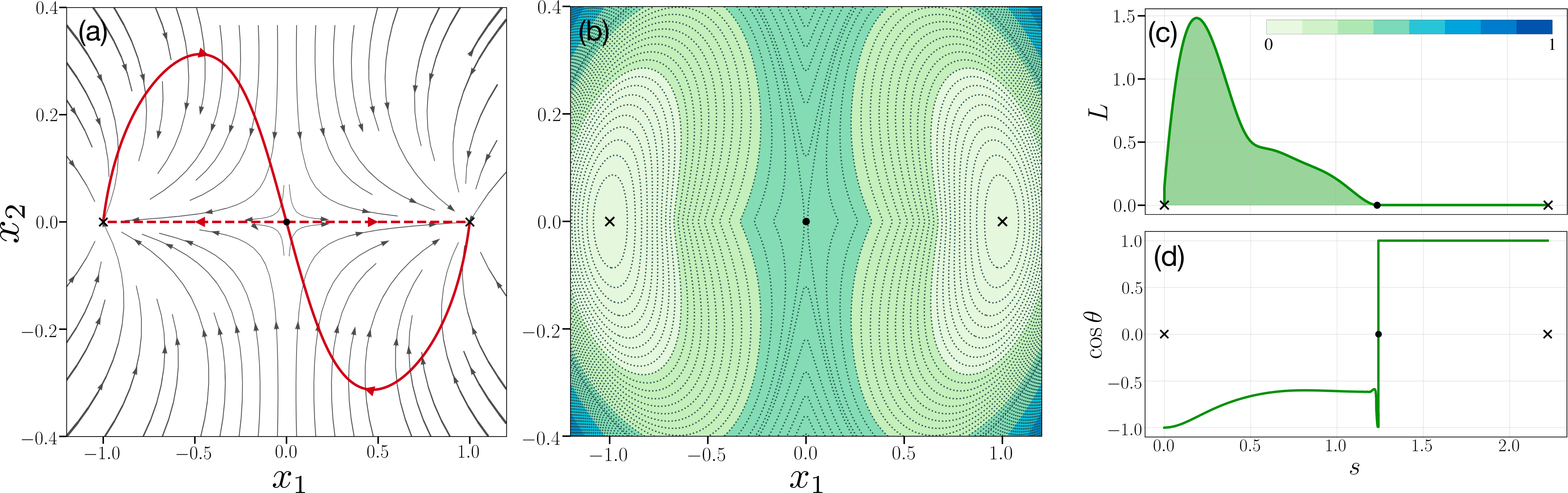
for the overdamped motion of the two-dimensional coordinate , where is a parameter. The force field is smooth, and is odd in and even in , while for the converse holds. There are two stable fixed points at and , and a saddle point at . The force field admits a potential only for , when it can be written as , with . The force field is shown in the first panel of Fig. 2 for together with the instanton moving from to . As before, solid (dashed) segments represent motion against (along) the vector field. The instanton moving from to is obtained by reflection about the -axis showing that that fluctuational and relaxational paths are not identical in a non-gradient field.
The middle panels shows the stationary quasipotential with respect to the attractors at and respectively. The quasipotential is sampled on a grid by computing instantons between a point on the grid and the relevant attractor. The contours of the quasipotential and its heatmap are obtained from these discrete samples. To the best of our knowledge, all prior estimations of the quasipotential for this problem (and more generally, for circulatory forces) have required numerical solutions of the Hamilton-Jacobi equation. Our method of direct sampling provides an alternative to this route of computing the quasipotential. The right panel shows the Lagrangian as a function of arc-length along the instanton. As in the previous example, the Lagrangian vanishes along segments of the path where motion is along the force. For motion against the force, the tangent to the path is no longer parallel to the force, as shown by the variation of the cosine of the angle between the tangent and the force. We note that our method is agnostic to the existence, or not, of a potential for the drift and treats both these cases on equal footing.
V.3 Egger model of weather
Our final example is a reduced model of the weather for a a three-dimensional coordinate that has a circulatory drift,
| (43) |
where , , , and are constants. This model is due to Egger (Egger 1981). It is not particularly illuminating to visualise the three-dimensional vector field describing this dynamics but we note that it has two stable fixed points, marked by crosses in Fig. 3, and a saddle fixed point marked by a dot. The instanton moving between these points is shown as before in the left and right panels of the figure. Also shown are isosurfaces of the quasipotential with respect to the stable fixed points, with isovalues increasing from red to blue. To the best of our knowledge, this is the first computation of the quasipotential for this model. We provide this example primarily to demonstrate the feasibility of sampling quasipotentials in dimensions greater than two with our method.
| Model | |||||
|---|---|---|---|---|---|
| M-B | |||||
| M-S | |||||
| Egger |
VI Numerical convergence
We briefly recall the convergence properties of the Ritz method, comprising that of the basis functions, the quadrature, and the optimisation. The Chebyshev interpolant is guaranteed to converge to the most probable path, assuming that it is Lipschitz continuous, at a rate that increases with the number of derivatives the path admits and is exponential for a smooth path. Likewise, the Clenshaw-Curtis quadrature is guaranteed to converge to the minimum of the action, assuming that the Lagrangian is Lipschitz continuous. The optimal number of quadrature points for accuracy to machine precision can be obtained by following the decay of the Chebyshev coefficients of the Lagrangian and truncating at that value beyond which the coefficients vanish to machine precision. The optimisation has lesser theoretical guarantees than the interpolation and quadrature, as is generally the case with search in high-dimensional spaces. However, the residual of the Ritz system provides an empirical measure for how closely the minimum has been located. In all three examples (and in others not presented here) we have found both gradient-free and gradient-based optimization to robustly locate the minima, and gradient-based methods to yield faster convergence. We note that for equilibrium problems, the gradient-free method does not require the Hessian of the energy function, which can be of significant computational advantage. In Table 1 we show the spectral convergence of the action with increasing polynomial order of the path for each of our examples.
VII Discussion
We have presented an efficient and accurate numerical method for computing most probable transitions paths and quasipotentials of rare diffusive events. The method directly minimises the Freidlin-Wentzell action and thus provides an unified approach for transition paths in both equilibrium and non-equilibrium systems. Our reparametrisation-invariant form of the action, derived using a Noether symmetry, is well-suited for numerical work and is a generalisation of the geometric action. This frees us from the constraints of the commonly used arc-length path parametrisation and offers the maximum flexibility in choosing the space of polynomials in which action is minimised. Thus our method is not limited to the Chebyshev polynomials in used here but easily admits trigonometric polynomials and, more generally, any global basis. Numerical quadrature reduces the action to a multivariate function of coefficients of the path polynomial whose minimum is obtained by both gradient-free and gradient-based optimisation. This gives, simultaneously, both the minimum value of the action and the most probable path. This efficiency of the method allows us to repeatedly compute minimum action paths between an attractor and a point in its basin of attraction and, thereby, map out the quasipotential. The quasipotential in a non-equilibrium steady state has the same significance as the Gibbs distribution in equilibrium and our method provides a robust way of obtaining it without the need to numerically solve the Hamilton-Jacobi partial differential equation.
The direct method used here consists of a discretisation of the action followed by a search for the minimum in the resulting finite-dimensional space, expressed schematically in Fig. (4). In contrast, the majority of methods impose the vanishing variation of the action and then search for the solution of the Euler-Lagrange equation in a finite-dimensional space. The resulting discretised Euler-Lagrange equations is, in general, not identical to the Ritz system; in other words, these two methods of reducing an infinite-dimensional problem to a finite-dimensional one are not equivalent. In contrast to mechanics, where Newton’s equations of motion are considered primary and the action derived, here it is the tube probability and hence the Freidlin-Wentzell action that is primary and the Euler-Lagrange equation for the most probable path that is derived. It appears more natural to us to discretise the primary, rather than the derived, object directly. Our approach is algorithmically simple and the only adjustable parameters are the polynomial order and the quadrature order This simplicity does not compromise accuracy or efficiency, as confirmed by our examples.
The rapid convergence of the method holds promise for its application to problems involving the stochastic dynamics of fields, with both scalar and Lie group-valued order parameters. We also expect the method to apply to stochastic dynamics with degenerate diffusion tensors and to stochastic systems with inertia. These will be addressed in forthcoming work.
VIII Acknowledgements
We thank Julian Kappler for many helpful discussions. Work funded in part by the European Research Council under the Horizon 2020 Programme, ERC grant agreement number 740269. RS is funded by a Royal Society-SERB Newton International Fellowship. MEC is funded by the Royal Society.
References
- Wentzell and Freidlin (1970) A. D. Wentzell and M. I. Freidlin, Russian Mathematical Surveys 25, 1 (1970).
- Bolhuis et al. (2002) P. G. Bolhuis, D. Chandler, C. Dellago, and P. L. Geissler, Annual Review of Physical Chemistry 53, 291 (2002).
- Allen et al. (2005) R. J. Allen, P. B. Warren, and P. R. Ten Wolde, Physical Review Letters 94, 018104 (2005).
- Allen et al. (2009) R. J. Allen, C. Valeriani, and P. R. ten Wolde, Journal of Physics: Condensed Matter 21, 463102 (2009).
- Ebener et al. (2019) L. Ebener, G. Margazoglou, J. Friedrich, L. Biferale, and R. Grauer, Chaos: An Interdisciplinary Journal of Nonlinear Science 29, 063102 (2019).
- Paninski (2006) L. Paninski, Journal of Computational Neuroscience 21, 71 (2006).
- Huang (2012) S. Huang, Bioessays 34, 149 (2012).
- Bouchet and Reygner (2016) F. Bouchet and J. Reygner, in Annales Henri Poincaré, Vol. 17 (Springer, 2016) pp. 3499–3532.
- Maier and Stein (1996) R. S. Maier and D. L. Stein, Journal of Statistical Physics 83, 291 (1996).
- Wolynes et al. (1995) P. Wolynes, J. Onuchic, and D. Thirumalai, Science 267, 1619 (1995).
- Nolting and Abbott (2016) B. C. Nolting and K. C. Abbott, Ecology (2016).
- Mangel (1994) M. Mangel, Theoretical Population Biology 45, 16 (1994).
- Gardner et al. (2000) T. S. Gardner, C. R. Cantor, and J. J. Collins, Nature 403, 339 (2000).
- DeMarco (2001) C. L. DeMarco, IEEE Control Systems Magazine 21, 40 (2001).
- Nelson (1987) R. Nelson, Journal of the ACM (JACM) 34, 661 (1987).
- Weinan et al. (2002) E. Weinan, W. Ren, and E. Vanden-Eijnden, Physical Review B 66, 052301 (2002).
- Heymann and Vanden-Eijnden (2008) M. Heymann and E. Vanden-Eijnden, Communications on Pure and Applied Mathematics 61, 1052 (2008).
- Grafke et al. (2017) T. Grafke, T. Schäfer, and E. Vanden-Eijnden, in Recent Progress and Modern Challenges in Applied Mathematics, Modeling and Computational Science (Springer, 2017) pp. 17–55.
- Gelfand and Fomin (2012) I. Gelfand and S. Fomin, Calculus of Variations, Dover Books on Mathematics (Dover Publications, 2012).
- Kantorovich and Krylov (1958) L. Kantorovich and V. Krylov, Approximate Methods of Higher Analysis (P. Noordhoff, 1958).
- Weinan et al. (2004) E. Weinan, W. Ren, and E. Vanden-Eijnden, Communications on Pure and Applied Mathematics 57, 637 (2004).
- Ritz (1909) W. Ritz, Journal für Mathematik 135, 1 (1909).
- Vanden-Eijnden and Heymann (2008) E. Vanden-Eijnden and M. Heymann, “The geometric minimum action method for computing minimum energy paths,” (2008).
- Cameron (2012) M. Cameron, Physica D: Nonlinear Phenomena 241, 1532 (2012).
- Yang et al. (2019) S. Yang, S. F. Potter, and M. K. Cameron, Journal of Computational Physics 379, 325 (2019).
- Dahiya and Cameron (2018) D. Dahiya and M. Cameron, Journal of Scientific Computing 75, 1351 (2018).
- Graham (1973) R. Graham, in Springer tracts in modern physics (Springer, 1973) pp. 1–97.
- Graham (1987) R. Graham, in Fluctuations and Stochastic Phenomena in Condensed Matter (Springer, 1987) pp. 1–34.
- Touchette (2009) H. Touchette, Physics Reports 478, 1 (2009).
- Ludwig (1975) D. Ludwig, Siam Review 17, 605 (1975).
- Whittaker (1988) E. T. Whittaker, A Treatise on the Analytical Dynamics of Particles and Rigid Bodies, Cambridge Mathematical Library (Cambridge University Press, 1988).
- Landau and Lifshitz (1959) L. Landau and E. Lifshitz, “Classical mechanics,” (1959).
- Gantmacher (1970) F. Gantmacher, Lectures in analytical mechanics.(Translated from the Russian by G. Yankovsky) (Moscow: Mir Publishers, 1970).
- Olender and Elber (1997) R. Olender and R. Elber, Journal of Molecular Structure: THEOCHEM 398, 63 (1997).
- Onsager and Machlup (1953) L. Onsager and S. Machlup, Physical Review 91, 1505 (1953).
- Stratonovich (1989) R. Stratonovich, in IN: Noise in nonlinear dynamical systems. Volume 1 (A90-30467 12-70). Cambridge and New York, Cambridge University Press, 1989, p. 16-71., Vol. 1 (1989) pp. 16–71.
- Elsgolts and Yankovsky (1973) L. E. Elsgolts and G. Yankovsky, Differential equations and the calculus of variations (Mir Moscow, 1973).
- Gander and Wanner (2012) M. J. Gander and G. Wanner, Siam Review 54, 627 (2012).
- Trefethen (2000) L. N. Trefethen, Spectral methods in MATLAB, Vol. 10 (Siam, 2000).
- Boyd (2001) J. P. Boyd, Chebyshev and Fourier spectral methods (Courier Corporation, 2001).
- Trefethen (2013) L. N. Trefethen, Approximation theory and approximation practice, Vol. 128 (Siam, 2013).
- Hamming (2012) R. Hamming, Numerical methods for scientists and engineers (Courier Corporation, 2012).
- Salzer (1972) H. E. Salzer, The Computer Journal 15, 156 (1972).
- Berrut and Trefethen (2004) J.-P. Berrut and L. N. Trefethen, SIAM review 46, 501 (2004).
- Aurentz and Trefethen (2017) J. L. Aurentz and L. N. Trefethen, ACM Transactions on Mathematical Software (TOMS) 43, 33 (2017).
- Powell (2006) M. J. Powell, in Large-scale nonlinear optimization (Springer, 2006) pp. 255–297.
- Kraft (1988) D. Kraft, Forschungsbericht / Deutsche Forschungs- und Versuchsanstalt fur Luft- und Raumfahrt 88–28 (1988).
- Johnson (2014) S. G. Johnson, “The nlopt nonlinear-optimization package,” (2014).
- Müller and Brown (1979) K. Müller and L. D. Brown, Theoretica chimica acta 53, 75 (1979).
- Egger (1981) J. Egger, Journal of the Atmospheric Sciences 38, 2606 (1981).