The Structure of Radiatively Inefficient Black Hole Accretion FlowsAthena++ (White et al. 2016), ibothros (Noble et al. 2007)
Abstract
We run three long-timescale general-relativistic magnetohydrodynamic simulations of radiatively inefficient accretion flows onto non-rotating black holes. Our aim is to achieve steady-state behavior out to large radii and understand the resulting flow structure. A simulation with adiabatic index and small initial alternating poloidal magnetic field loops is run to a time of , reaching inflow equilibrium inside a radius of . Variations with larger alternating field loops and with are run to , attaining equilibrium out to and . There is no universal self-similar behavior obtained at radii in inflow equilibrium: the simulation shows a radial density profile with power law index ranging from in the inner regions to in the outer regions, while the others have a power-law slope ranging from to close to . Both simulations with small field loops reach a state with polar inflow of matter, while the more ordered initial field has polar outflows. However, unbound outflows remove only a factor of order unity of the inflowing material over a factor of in radius. Our results suggest that the dynamics of radiatively inefficient accretion flows are sensitive to how the flow is fed from larger radii, and may differ appreciably in different astrophysical systems. Millimeter images appropriate for Sgr A* are qualitatively (but not quantitatively) similar in all simulations, with a prominent asymmetric image due to Doppler boosting.
I Introduction
A common mode of accretion onto black holes is that of a radiatively inefficient accretion flow (RIAF). Such systems have nonzero net angular momentum, as opposed to classical Bondi accretion (Bondi 1952), but because of inefficient cooling they are dynamically hot, thick disks (Ichimaru 1977; Rees et al. 1982; Narayan & Yi 1995), unlike standard thin disk models (Shakura & Sunyaev 1973). RIAFs are consistent with a number of low-luminosity active galactic nuclei, including Sgr A* (Narayan et al. 1998).
Simulations of black hole accretion on horizon scales, where general relativity (GR) cannot be neglected, are almost always initialized as hydrostatic equilibrium torus solutions with simple angular momentum prescriptions (Fishbone & Moncrief 1976; Kozłowski et al. 1978; Chakrabarti 1985; Penna et al. 2013). While such simulations tend to reach a well-defined quasi-steady state in the inner portions of the flow, there is still an open question as to how much this state depends on the fact that the simulations begin with a relatively artificial initial condition.
In thin accretion disks there is a large timescale separation between the viscous and dynamical times and rapid radiative cooling enables the flow to lose memory of its initial thermodynamic state. This is much less true in RIAFs, so one might expect the dynamics of such flows to retain more memory of how the matter is fed to the vicinity of the black hole from larger radii. There are a number of analytic models for the structure of RIAFs, which differ primarily in the importance of non-radiative energy transport mechanisms, e.g. advection, convection/turbulence, and outflows (Narayan & Yi 1994; Blandford & Begelman 1999; Quataert & Gruzinov 2000; Narayan et al. 2000). It is unclear which, if any, of these is a correct description of RIAFs or whether different non-radiative energy transport mechanisms are important depending on how matter is fed to the vicinity of the black hole.
Previous work has shown that the flow structure at small radii in black hole accretion simulations depends on the magnetic field structure threading the initial torus, in particular how much magnetic flux there is at a given radius and/or through the whole torus (Narayan et al. 2003; Beckwith et al. 2008). The initial field structure influences both the strength of the resulting jet and whether the dominant angular momentum transport is produced by small-scale turbulent stresses due to the magnetorotational instability or by large-scale magnetic stresses.
One of the computational challenges in studying the connection between the small and large-scale flow structure is that the region in steady state grows outward only sublinearly with simulation time. Here we address this challenge with the brute-force method of long timescale simulations that reach steady state over as extended a radial range as possible. We then attempt to address whether a well-defined self-similar state is reached at small radii independent of initial conditions.
The idea of running GR simulations for long times to achieve steady state over large distances has been pursued before, notably by Narayan et al. 2012.11 1 Stone et al. 1999, Igumenshchev & Abramowicz 2000, and Yuan et al. 2012 studied the radial structure of RIAFs using axisymmetric hydrodynamic simulations with an viscosity, with outcomes differing with the details of that viscosity. The differences between hydrodynamic and magnetohydrodynamic (MHD) simulations make it difficult to know how to connect the results of those simulations to the MHD problem considered here. They considered two instances of RIAF flows: a disk with standard and normal evolution (SANE), and a magnetically arrested disk (MAD). Their initial conditions differ only in whether the purely poloidal magnetic field has the topology of a single loop in a slice of constant azimuth, conducive to accumulating net vertical magnetic flux and inducing a MAD state, or else has multiple loops and thus stays in the SANE regime. Their SANE simulation reaches steady state out to about gravitational radii after running for a time .
Here we focus on the SANE case, primarily because such models are a priori more similar to the self-similar analytic models that still guide much of the intuition in thinking about RIAF structure across many decades in radius. We extend Narayan et al. 2012’s work by running three variations on the initial conditions to probe how the final state is sensitive to details of the initial state, with the longest simulation run for a time . The numerics and setup of the simulations are detailed in §II. We present accretion rates and related global quantities in §III and radial profiles of quantities in steady state in §IV. The global inflow and outflow structure is analyzed in §V, and observational consequences are discussed in §VI. Our conclusions are summarized in §VII.
Throughout this work, all length scales will be expressed in implicit units of gravitational radii , where is the black hole mass. Likewise times will be in units of and velocities in units of , with units derived from these following naturally. The magnetic field contains an implicit factor of , so for example the magnetic pressure is given by if the components are measured in a Minkowski frame comoving with the fluid.
II Numerical Setup
We perform our simulations with the GRMHD code Athena++ (White et al. 2016). The code uses a second-order van Leer integrator at a Courant–Friedrichs–Lewy number of , where is the maximum stable value for this integrator in three spatial dimensions, along with second-order modified van Leer spatial reconstruction from Mignone 2014. Fluxes are calculated via the HLLE Riemann solver.
While less diffusive Riemann solvers such as HLLD exist for relativistic MHD (Mignone et al. 2009), we choose HLLE based on two considerations. First, shocks in HLLD are narrowed to be only one or two cells thick. In a multidimensional finite-volume method, such steep gradients can lead to the conserved variables in a cell entering a physically inadmissible state during a single timestep, manifesting as a variable inversion failure when trying to recover the primitive variables. Given that these simulations need to take tens of millions of timesteps, we want to minimize the chance of catastrophic inversion failures. Second, HLLE is common practice in the GRMHD community. For example, in the recent code comparison of Porth et al. 2019, which includes Athena++, the nine codes exclusively employ either HLLE or the more diffusive LLF Riemann solver, yet they are able to reach agreement with sufficient resolution. HLLD would enable us to resolve the same phenomena with fewer cells, but we are willing to use HLLE with higher resolution here in order to achieve robustness over very long integration times.
Spacetime is fixed to be that of a nonspinning black hole, . The simulations employ spherical Kerr–Schild coordinates with volume element . Our coordinate system covers the entire sphere, including the appropriate transmissive polar boundary. In the radial direction the cell boundaries are logarithmically spaced from (inside the horizon) to . In the poloidal direction we compress the cells near the equatorial plane as in Gammie et al. 2003 (except we adjust cell spacing rather than the metric). The result is that cells are uniformly spaced in a midplane-compressed coordinate related to the standard via
| (1) |
Due to the particularly long integration times required for these simulations, we additionally use static mesh refinement to keep the part of the grid near the poles at low resolution. The root grid consists of cells in the radial, polar, and azimuthal directions respectively. The region is refined by a factor of in each dimension, and the region is refined by a factor of relative to the root grid. The cells at the midplane thus have thickness .
The initial conditions are those of the hydrostatic equilibrium solution of Fishbone & Moncrief 1976 with a pressure maximum at and a peak density of . The latter sets an arbitrary scale for the fluid mass, which is taken to be negligible compared to the black hole mass. Simulations A and B have an inner edge at and an adiabatic index of , while simulation C has an inner edge at and . Indices of and are approximations to the thermodynamics appropriate for super- and sub-Eddington RIAFs, respectively. The slight change of inner edge radii helps to make the extent of the mass distribution of simulation C similar to that of the other two. The resulting densities are shown in Figure 1, with the midplane run of with radius on the top and a vertical slice on the bottom.
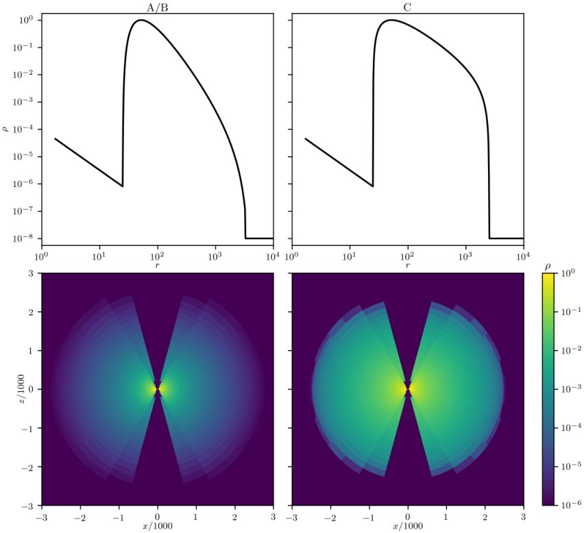
We add a weak magnetic field to this initial torus. The field is derived from the purely azimuthal vector potential with component
| (2) |
where is the gas pressure and is a linear ramp function:
| (3) |
The form of this function is chosen to allow for a variable number of counterrotating loops in both directions, and to give roughly constant values for plasma , the ratio of magnetic to gas pressure. We choose the parameters , , , , and in all simulations. For simulations A and C we have and , while in simulation B we set and . In all cases the field strength is normalized such that
| (4) |
where the integrals exclude the background atmosphere outside the torus. These field configurations are illustrated in Figure 2.

Finally, we perturb the initial velocities inside the torus as follows. We consider the normal observer velocity components , where is a component of the standard shift. We introduce small motions in the poloidal directions according to
| (5a) | ||||
| (5b) | ||||
where and are standard cylindrical coordinates. We choose and .
Simulation A is run to , while the variations and are run to . The cost of these runs is approximately core-hours per simulation time unit (Intel Xeon E5-2670 CPU) or core-hours per time unit (Intel Xeon Platinum 8160 CPU).
III Accretion Rates
We follow Narayan et al. 2012 and divide the simulations into logarithmic chunks in time. The eight boundaries of these seven chunks are , , , , , , , and . We will use a consistent color scheme to label these chunks throughout all figures.
The mass accretion rate is defined in the usual way, integrating over a spherical shell:
| (6) |
The run of the horizon value of with time is given in Figure 3. As can be seen in the figures, the first time chunks are chosen to be well after the initial transience. Simulations A and B begin depleting their mass reservoir, while simulation C has much more mass and so only shows signs of decreasing at the very end of the run. By the end of chunk 5 (), simulations A, B, and C have lost , , and of their initial masses, with , , and of the original mass going through the horizon. After simulation A has run for twice as long, it has lost a total of of its mass, with going into the black hole. Some of this mass loss is due to bulk outflows originating from smaller radii (discussed in §V), while the rest comes from the outer parts of the initial torus moving outward as they receive angular momentum from the inner parts. In Simulation A, the accretion rate approaches a scaling of at very late times, as shown by the dotted line. This is the expected scaling for a RIAF in the absence of outflows removing mass or angular momentum. Since the simulation has outflows and is probably not fully in the asymptotic regime where would be expected, it seems likely that the agreement between the simulation and this analytic expectation is fortuitous.
We can also look at as a function of radius. This is done in Figure 4, where the separate lines are time averages over different chunks. In steady state we expect these values to be close to constant out to some radius, and indeed they are even as this constant decreases with time. The flatness of the curves at the inner radii indicates the solution is in a quasi-steady state and that numerical density floors do not play a large role in the inner parts of the simulations.
For later analysis, we use the vs. radius curves to define a “viscous radius” inside of which the system has reached inflow equilibrium. We choose the point where drops to times its horizon value. These radii are delineated by the points in Figure 4. The range over which equilibrium is established does indeed move outward in time, extending to in chunk 7 of simulation A and to and in chunk 5 of simulations B and C. For a constant and constant model we would expect the viscous radius to move outward in time as . The numerical evolution is generally slower than this, as we discuss further below in §IV.
The energy accretion rate is very similar to the total mass accretion rate. Define
| (7a) | ||||
| (7b) | ||||
where the stress-energy tensor is given by
| (8a) | ||||
| (8b) | ||||
| (8c) | ||||
| (8d) | ||||
| (8e) | ||||
| (8f) | ||||
Runs of and with radius, averaged in time over chunk 5, are shown in Figure 5. The other time chunks show essentially the same behavior. The overall energy accretion rate tracks mass very closely. This is to be expected, since rest mass density dominates over gas pressure as well as the contribution of the electromagnetic field. That is, we are mostly measuring rest mass being advected into the black hole. The electromagnetic contribution to the flux of energy, shown by the dotted line, is negative, indicating an outflow. However the magnitude of this component is only one part in a thousand of the total. This would be significantly larger for a spinning black hole.
Just as with mass and energy we monitor the flux of angular momentum, defining
| (9) |
This is also shown in Figure 5. Again we see the radially constant plateaus indicating approximate steady state, though the deviations begin at slightly smaller radii than for . The steady-state value of does not change with magnetic field topology (cf. simulations A and B), but does change in the case of a different (simulation C).
We additionally calculate the horizon-penetrating flux
| (10) |
This is the same quantity as defined in Tchekhovskoy et al. 2011 and Narayan et al. 2012, where our explicit factor of is implicit in their units, except here we use the instantaneous not convolved with any smoothing kernel in time. The run of with time in the two simulations is shown in Figure 6. Simulations A and C, with their small initial field loops (see Figure 2), stay very much in the SANE regime, with at late times. For comparison, the MAD simulations in Tchekhovskoy et al. 2011 have . Simulation B goes through a burst of higher flux, though it does not stay high as in a true MAD disk. The behavior of simulation B matches that of the SANE simulation in Narayan et al. 2012, which uses a similar initial field topology.
IV Radial Profiles in the Disk
We now turn to characterizing the properties of the disks, starting with profiles of disk properties as functions of radius.
We define the spherical scale height at a radius to be
| (11) |
where the integrals are taken over spheres at that radius. The run of this quantity with radius, averaged within time chunks, is shown in Figure 7. In all simulations, this scale height stays between approximately and , increasing toward larger radii and changing little over time. Simulation C, with , stays somewhat thicker at very small radii compared to the other cases.
With scale height in hand, we can define averages of quantities over the disk proper, here taken to be the region within one scale height of the midplane. The average density we define to be
| (12) |
Note that a more appropriate volume element might use the determinant of the metric restricted to hypersurfaces of constant , or even surfaces of constant and . However all these choices differ by factors that depend only on in the case of nonspinning black holes, and so they all lead to equivalent definitions of .
The profiles of density are shown in the upper panels of Figure 8, where the points indicate inflow equilibrium as defined in §III. The profiles generally approach power laws in radius, especially at very late times in simulation A. The very inner regions of simulations A and B, inside , have a shallower power-law slope when compared with the outer part of the viscous range. This is likely produced by the rapid acceleration needed close to the horizon: conservation of mass implies that the density profile flattens as the velocity accelerates. Somewhat surprisingly, simulation C does not display this knee, though it does have a slight persistent kink between and .
The lower panels of Figure 8 show the power-law slopes of the density profiles. Specifically, for an abscissa the ordinate is the slope of a linear regression to the set of points for which is within a factor of approximately of . The inner regions of simulations A and B have slopes of very roughly . The range over which this holds does not increase after a point, even at very late times as in simulation A. The middle of the inflow equilibrium range in simulation A eventually tends toward a slope of approximately at very late times. Simulation B does not reach sufficiently late times and does not show signs of converging to a constant slope. Simulation C, on the other hand, has a slope of between and over all radii in equilibrium. Analytic models of RIAFs predict power-law density profiles far from the horizon ranging from (Narayan & Yi 1994) to (Narayan et al. 2000; Quataert & Gruzinov 2000), and everything in between (Blandford & Begelman 1999). One might expect that there would be a well-defined self-similar state of the accretion flow that obtains at radii , where the impact of the black hole horizon on the flow structure is no longer significant. The density profiles in Figure 8 are not consistent with this ansatz. Instead, the profiles depend on the thermodynamics, parameterized by adiabatic index here, and initial magnetic field structure.
We can average other quantities in a density-weighted way. For any quantity other than , define
| (13) |
Although not shown explicitly here, all three accretion flows are slightly sub-Keplerian, as can be seen by examining for Boyer–Lindquist angular velocity . The average infall velocity , where , is well below the free-fall value.
The averages of magnetization are given in Figure 9. Magnetization decreases with increasing radius out to in all simulations, but it remains relatively flat beyond that in cases A and B, even when equilibrium is established much further out. The levels of these flat portions can change in time, however, first decreasing and then increasing at late times (simulation A). We note that simulations A and B, whose only difference is the initial field topology, reach the same profile of by the fourth time chunk, indicating that the saturated field strength may not strongly depend on details of initial conditions. In simulation C, the profile of levels off near where does, and then proceeds to again decrease with increasing radius beyond that.
The increased magnetization at small radii influences the rates at which our viscous radii move outward. Given the scaling , and given the observed thicknesses (Figure 7), we might expect equilibrium to be established out to a radius by time . However the radii marked in Figure 4 do not advance in time this rapidly. For example, chunks 1 and 7 are separated by a factor of in time, while equilibrium is only established times further out in the latter compared to the former for simulation A. This can be explained by noting we also expect , and . Thus , and so equilibrium is established much more rapidly at small radii with strong magnetization than at large radii.
V Global Structure of the Accretion Flow
Going beyond radial profiles, we show the late-time magnetic field in the poloidal plane in Figure 10, superimposed on the time-averaged density. This magnetic field is obtained by averaging and in azimuth and averaging in time over the last common time chunk (5) available for all simulations. It shows what steady-state structure arises from the initial fields in Figure 2.

We can immediately see that simulation A has a more ordered, radial field near the midplane when compared to the other two cases, despite simulation C having the same initial field topology. This can be explained by the velocity structure of the flows, discussed below. Simulation A also shows near cancellation in vertical fluxes at fixed radius; i.e. is antisymmetric across . Simulation B, on the other hand, shows a field topology with symmetric across the midplane. While the net flux integrated over a large radial extent may vanish, there is generally net flux at any given radius. These symmetries are also found in the initial conditions, indicating that even at these late times the initial field’s imprint on the field topology remains. It is also striking how spherical the density distribution is in Simulation C: there is only a factor of few variation in density from equator to pole. By contrast simulations A and B show the more “standard” disc structure of a dense midplane and a low-density polar region.
The net accretion rates shown in Figures 3 and 4 do not fully describe the radial motion of matter, since there can be outflows partially negating mass inflow elsewhere. While this will certainly happen over small time and length scales due to turbulence, coherent outflows may persist even when averaged over turbulence.
Indeed, we do observe large-scale outflows in our simulations, particularly with more ordered magnetic fields. Figure 11 shows the velocity field for each simulation in the poloidal plane, averaged in azimuth with density weighting and again averaged over the last common time chunk. Simulation B shows an accretion disk with a low radial velocity, together with fast, low-density, polar outflows. This is similar to the now-canonical assumed structure of RIAFs from earlier simulations (e.g., Hawley & Balbus 2002). Simulations A and C, however, show the reverse. In these cases matter is falling in through the poles, with outflow occurring in the disk. This disk outflow pattern is particularly strong in simulation A.

We can further decompose into ingoing and outgoing components based on radial mass fluxes that have been averaged in time and azimuth:
| (14a) | ||||
| (14b) | ||||
The runs of these quantities with radius are given in Figure 12. We know must be constant in radius from Figure 4, and indeed is close to constant, with being a small perturbation over most of the viscous range. The fact that becomes negligible inside in simulations A and C tells us that the disk outflows we observe (see Figure 11) do not extend all the way to the horizon. In simulation B, also drops off at small radii, matching how the polar outflow shown in Figure 11 reaches a stagnation surface at . Our results on the disk outflows are broadly consistent with Narayan et al. 2012, who also find that outflows were at most an order unity perturbation to the accretion rate for the radial range they simulate.
What is the physical origin of the outflows seen in Figure 12 and the flow structure seen in Figure 11? Two possible hydrodynamic mechanisms for large-scale flows of this kind are convection and meridional circulation. We examine these quantitatively in Appendix A and find that they are not very compelling in explaining our numerical results.
The fact that both simulations A and C display polar inflows and disk outflows despite having different values of and different initial tori indicates this phenomenon is not limited to a small set of hydrodynamic initial conditions. Simulations A and B, meanwhile, have identical hydrodynamic initial conditions yet vastly different steady-state velocity structures. This points to the original magnetic field topology as being important in determining the inflow and outflow structure (as was emphasized by, e.g., Beckwith et al. 2008).
As discussed in §II, the initial field in simulation B consists of elongated loops in the poloidal plane (see Figure 2). While there is no net vertical flux when averaged over sufficiently large radial extents, there is net flux at any given radius. Thus accretion brings a sequence of alternating net fluxes to the black hole over time (Figure 6), causing bursts in accretion rate (Figure 3). While the black hole has no spin and thus there are no Blandford–Znajek jets (Blandford & Znajek 1977), the net flux in the disc may be enough to drive a polar outflow via the Blandford–Payne mechanism (Blandford & Payne 1982) or related MHD processes. This can prevent any loosely bound polar inflow coming in from the disk at larger radii from reaching the black hole.
Simulations A and C, on the other hand, have no net flux at any radius. It is more difficult for the magnetic field in these cases to launch polar outflows, and so material can fall to the black hole near the polar axes. With enough polar inflow, the liberated gravitational potential energy can help to unbind material, driving it outward in the equatorial plane.
We quantify the extent to which material is bound with the Bernoulli parameter, which we define as
| (15a) | ||||
| (15b) | ||||
with averages being taken in azimuth and time. This is similar to equation (11) of Narayan et al. 2012. Plots of for the last common time chunk of each simulation are given in Figure 13. Note throughout the initial tori.

We see that most of the disks in all three cases have become unbound. At the same time, the polar regions of simulations A and C are bound, while they are very much unbound in simulation B. The initial magnetic field topology thus has a strong effect on the overall energetics and dynamical structure of RIAFs. This occurs primarily, we believe, via the energy redistribution and outflows associated with magnetic stresses, not just the angular momentum transport they produce.
Evidence for this comes from the fact that over a large range of radii all three simulations have similar radial accelerations, vanishing near the midplane and directed inward at high latitudes. The presence of a narrow outflow along the polar axis, for instance, is not due to consistent, outward, electromagnetic acceleration along the axis, but rather to the combined effect of accelerations at other locations. We quantify these accelerations by writing the inhomogeneous geodesic equation for a perfect fluid as
| (16a) | ||||
| (16b) | ||||
| (16c) | ||||
| (16d) | ||||
where is the projection operator relative to the fluid velocity. Figure 14 shows the radial components of these three forces along an arc of constant radius , computed from the fluid state obtained by averaging in time and azimuth over chunk 5. The gravitational (including centrifugal) force is closely balanced by the gas pressure gradient; the magnetic pressure gradient and Maxwell stress are both small. In simulation A but not in simulation C, there may be some ongoing outward radial acceleration near the upper and lower disk surfaces. In these locations approaches , indicating a large centrifugal force nearly balancing gravitational attraction even without pressure support.
Appendix B shows the steady-state behavior of two additional runs, paralleling simulations A and B in how their initial fields differ but using a smaller initial torus. The dichotomy between polar inflows and outflows persists, with inflows occurring where there is no local net vertical flux in the initial conditions. These smaller tori, which are closer in size to those most often employed in the literature, are more tightly bound, and so even the case with polar inflow does not develop an equatorial outflow. The latter result highlights that conclusions drawn from small torus simulations might be inaccurate in some cases.
VI Observational Consequences
Given the length of time we have run these simulations, we have a large amount of data on their time variability. In particular, for simulation A we have high-cadence samples of the horizon value of sampled with a time interval . For a Sgr A*-like mass of , this corresponds to a sampling period of .
We construct the power spectrum of the time series using Welch’s method on overlapping segments of time durations ranging from (used to calculate a smooth spectrum at high frequencies) to (used at low frequencies), applying a Hann window to each segment. An overall linear trend in the quantities and is subtracted before calculating each spectrum. We do this for the union of chunks 6 and 7. The results are shown in Figure 15. Here we refer to as the power, where is the power per unit frequency.
The spectrum has a slope over the range , somewhat steeper than ideal red noise. The slope is if we analyze chunks 1–5 instead of 6 and 7. A turnover to a flat spectrum is apparent at approximately , especially in simulation A. Simulations B and C have similar spectra at low frequencies, both in amplitude and slope. However, their values are only sampled every time units, and so we cannot measure their spectra at frequencies above .
Numerical models of RIAFs have been widely used to predict event-horizon-scale emission and images. Such models form the basis for interpreting Event Horizon Telescope images of M87 (The Event Horizon Telescope Collaboration 2019a; The Event Horizon Telescope Collaboration 2019b; The Event Horizon Telescope Collaboration 2019c) and Sgr A*. Since our simulations provide three different realizations of the near-horizon structure of RIAFs, it is valuable to assess whether their predictions for the near-horizon emission differ. To do so, we employ the code ibothros (Noble et al. 2007) to generate images of synchrotron emission at in post processing. We take snapshots from chunk 5, separated by . For each one, we assume thermal synchrotron radiation from the electrons, with a simulation-to-electron temperature ratio of . The density scale of the simulation is adjusted to match the observed flux of of Sgr A* (Doeleman et al. 2008) assuming we are viewing the disk edge-on.
Figure 16 displays the average image resulting from stacking the frames for each model. Simulation A shows the most extended disk component outside the typical bright ring around the circular dark region. This equatorial component is most compact in simulation C, brightening the ring but not increasing its width on the approaching side of the disk. These differences can be understood via the average density and temperature structures in the flows. Case C has the steepest density profile in the inner region (Figure 8), as well as higher temperatures (as can be seen in the larger scale height, Figure 7). Thus the emission we see will be dominated by a small region near the photon orbit, slightly spread out along the ring but not radially. In contrast, case B and especially case A have emission from a wider range of radii near the disk midplane.

VII Conclusion
We have run and analyzed three long timescale simulations of RIAFs around non-spinning black holes. Building on Narayan et al. 2012 (see also related hydrodynamic work by Yuan et al. 2012) our goal has been to understand whether a well-defined self-similar structure of the accretion flow develops that is independent of the simulation initial conditions, and whether such a state is described by existing analytic models of RIAFs. All of our simulations are “SANE,” i.e. they do not have significant net magnetic flux over an appreciable range of radii. We run a fiducial simulation (A) with small alternating field loops (see Figure 2) and adiabatic index to . Variations with either larger loops (B) or (C) are run to . Note that and are rough approximations to super- and sub-Eddington RIAFs, respectively. The simulations reach inflow equilibrium, defined here as where falls to of its horizon value, past , , and , respectively. Energy and angular momentum fluxes are as constant with radius as mass fluxes over much of this range. We note that many of our principal conclusions are not unique to these long-timescale runs. On the contrary, Appendix B shows that they hold even for the smaller tori typically used in GRMHD simulations.
One of our principal results is that the dynamical structure of RIAFs is sensitive to initial conditions, at least over the time- and length-scales that we can afford to simulate. There is no evidence for a unique flow structure that loses memory of the initial conditions. This is not necessarily surprising given the lack of timescale separation among thermal, viscous, and dynamical times in RIAFs. Moreover, the absence of radiative cooling implies that the dynamics in RIAFs is particularly sensitive to modest changes in flow energetics (produced, e.g., by differences in magnetic field structure).
In more detail, Figure 8 shows that the simulations maintain shallow slopes in density of in the innermost regions, with slopes at least as steep as approximately in the outer regions that are still in steady state. In the case, we see slopes closer to in the inner regions and in the outer regions. In a given simulation, we find that there is no clear convergence of to a particular value in the steady state flow exterior to the inner , as might be expected if there were a unique self-similar solution for the structure of RIAFs. By contrast, such a well-defined radial profile is seen in hydrodynamic models of RIAFs (e.g., Stone et al. 1999; Yuan et al. 2012). It is unclear if this difference between the hydrodynamic and MHD models reflects the very different angular momentum and energy transport physics in the two different simulations or if our simulations still do not have sufficient dynamic range to reach a quasi self-similar state. We suspect the former.
The larger magnetic field loops in simulation B relative to simulation A (see Figure 2) result in buildup of coherent magnetic flux at the horizon. While this simulation does not stay in a MAD state, it shows signs of alternating between “semi-MAD” states with oppositely directed fluxes. This does not have a noticeable effect on radial profiles of scale height, density, or magnetization, but it can affect the velocity structure of the accretion flow. In particular, the coherent vertical flux is enough to drive polar outflows in simulation B, whereas both simulations A and C have polar inflow of material (Figure 11). The absence of polar outflows in Simulation C is particularly striking as the density profile becomes nearly spherical with only a factor of few density contrast between the equator and poles (Figure 10).
The polar inflows we find are not readily explained by models for convective stability or meridional circulation (see Appendix A). However even a small amount of inflow can release enough energy to unbind significant portions of the disk, which for RIAFs is at best marginally bound. This is likely why the flow structure is sensitive to the magnetic field initial conditions, since the latter influences the angular momentum and energy transport at essentially all times in the simulation. Overall, we find that unbound outflows change the horizon-scale accretion rate by only a factor of order unity relative to the accretion rate at (see Figure 12), consistent with Narayan et al. 2012.
The sensitivity of the flow structure and dynamics in our simulations to modest changes in initial conditions (all within the context of highly artificial initial conditions) suggests that there is likely to be significant variation in the properties of RIAFs in nature depending on exactly how matter is supplied to the vicinity of the black hole from larger radii. Understanding this better in future work would be very valuable and would impact problems as diverse as accretion in the Galactic Center from stellar winds (e.g., Ressler et al. 2018) to the growth of supermassive black holes by highly super-Eddington accretion (e.g., Begelman & Volonteri 2017). We note that our calculations assume a nonspinning black hole, and future work should explore whether spin exacerbates or mitigates the sensitivity to how matter is supplied.
Numerical models of RIAFs have been widely used to predict event-horizon-scale emission, variability and images, particularly in the context of the well-studied systems M87 (Dexter et al. 2012; Mościbrodzka et al. 2016; Mościbrodzka et al. 2017; Ryan et al. 2018; Chael et al. 2019, e.g.) and Sgr A* (Mościbrodzka et al. 2014; Ressler et al. 2017; Chael et al. 2018, e.g.). As a result, we have made preliminary attempts to understand the observational implications of the diversity of flow structure and dynamics we find in our RIAF simulations. Towards this end, we calculate the power spectrum of in time for simulation A, using high-cadence samples at time intervals of ( for ), shown in Figure 15. The spectral power goes as at high frequencies. Our data shows a turnover toward white noise () at low frequencies; such a turnover has been measured in the submillimeter emission of Sgr A*, occurring at a timescale of (Dexter et al. 2014). This timescale corresponds to a frequency in our geometric units of (for reference, this is the reciprocal of the orbital period at ), which is consistent with where we see the turnover in power.
Motivated by the Event Horizon Telescope, we also calculate millimeter images of synchrotron emission for parameters appropriate for Sgr A* (see Figure 16). All of our different realizations of RIAFs produce qualitatively similar images, dominated by a Doppler boosted region along with a faint ring (Figure 16). There are, however, interesting differences in the size of the emitting region and the prominence of the equatorial accretion disk, which is much less dominant in Simulation C () relative to Simulations A and B ().
Appendix A Analysis of Convection and Meridional Circulation
One possible cause of bulk outflows in disks is a stationary convection pattern. As described in Quataert & Gruzinov 2000 we can check for convective stability in the disk by examining the gradients of entropy and azimuthal velocity . We construct the quantity
| (A1) |
where , , and are defined by (A2–A4) of Quataert & Gruzinov 2000, using density-weighted averages of and in time and azimuth and using the last time chunk available to all simulations. Stability requires . The values for within one scale height of the midplane are shown in Figure 17. The two simulations with disk outflows, A and C, are slightly unstable against convection in the midplane, in contrast to simulation B, which is marginal. However simulation C is quite stable at slightly higher latitudes, where there is still a strong outflow. Thus convection does not seem to fully explain the different bulk patterns shown in Figure 11.

Classical convection is not the only way to achieve large-scale motions in a disk. A sufficiently small vertical stratification in entropy can lead to meridional circulation in which the material in the midplane of the disk moves outward, with inward flow through the coronal layers. Following the constant case presented in Philippov & Rafikov 2017 we define the circulation parameter
| (A2) |
where denotes . If this is positive we expect outflow in the midplane. is plotted for the same time chunks in Figure 18. In all three cases the values are positive throughout the disk. However, the values are similar for all three simulations; thus if this were the cause of the outflows in simulations A and C, we would expect it to lead to the same velocity structure in simulation B, which is not seen.
Appendix B Comparison with Smaller Tori
Here we briefly mention two additional setups that are run for comparison. These two variants on the same small initial torus show how slight changes in the initial magnetic field can lead to different velocity structures in steady state.
In both cases we start with a Fishbone & Moncrief 1976 torus around a nonspinning black hole with inner edge , pressure maximum , peak density , and adiabatic index . The grid extends inside the horizon and out to . At root level it contains cells, and we add three successive levels of mesh refinement, obtaining an effective resolution of within of the midplane.
The single-loop variant has a magnetic field initialized via
| (B1) |
while the multiple loops variant employs (2) with , , , , , , and . In both cases the normalization is such that the density-weighted average of is , and we perturb the initial state via (5) with and .
The single-loop variant is comparable to standard tori widely used in the literature, for example when testing and demonstrating a new GRMHD code (Gammie et al. 2003; Antón et al. 2006; White et al. 2016; Porth et al. 2017) or comparing such codes (Porth et al. 2019), though around a nonspinning black hole here. It is similar to a scaled-down version of simulation B. The other small torus is more akin to a scaled-down version of simulation A. The only difference between the two is the magnetic field configuration, which is chosen to remain SANE in both cases.
Due to their small size, we can run these tori through steady state and even through depletion (by for the single-loop case, slightly later with multiple loops) with relatively little computational expense. Figure 19 shows the run of with time in both cases.
Even with these widely used, standard, small tori, the final density and velocity structures depend on details of the initial field configuration. Density profiles, analogous to Figure 8, are shown in Figure 20, averaged in time over . Figure 21 shows the corresponding velocity structure, analogous to Figure 11. With a single loop, a relatively strong polar outflow is driven, even though there is no black hole spin, nor is a MAD state obtained. This reflects the behavior of simulation B, where some net vertical flux proves to be sufficient for launching polar outflows. On the other hand, the multiple-loops variant follows simulation A in having polar inflow at all radii.

The midplane in the multiple-loops small torus does not experience the same bulk outflow as simulation A. However, this can be attributed to larger Fishbone & Moncrief 1976 tori being less bound. The polar inflows in simulation A could unbind most of the accretion disk, while the inner parts of the multiple-loops disk can still flow inward despite the liberation of gravitational potential energy nearby.
References
- Antón et al. (2006) Antón, L., Zanotti, O., Miralles, J. A., et al. 2006, The Astrophysical Journal, 637, 296, doi: 10.1086/498238
- Beckwith et al. (2008) Beckwith, K., Hawley, J. F., & Krolik, J. H. 2008, The Astrophysical Journal, 678, 1180, doi: 10.1086/533492
- Begelman & Volonteri (2017) Begelman, M. C., & Volonteri, M. 2017, Monthly Notices of the Royal Astronomical Society, 464, 1102, doi: 10.1093/mnras/stw2446
- Blandford & Payne (1982) Blandford, R., & Payne, D. 1982, Monthly Notices of the Royal Astronomical Society, 199, 883, doi: 10.1093/mnras/199.4.883
- Blandford & Znajek (1977) Blandford, R., & Znajek, R. 1977, Monthly Notices of the Royal Astronomical Society, 179, 433, doi: 10.1093/mnras/179.3.433
- Blandford & Begelman (1999) Blandford, R. D., & Begelman, M. C. 1999, Monthly Notices of the Royal Astronomical Society, 303, L1, doi: 10.1046/j.1365-8711.1999.02358.x
- Bondi (1952) Bondi, H. 1952, Monthly Notices of the Royal Astronomical Society, 112, 195, doi: 10.1093/mnras/112.2.195
- Chael et al. (2019) Chael, A., Narayan, R., & Johnson, M. D. 2019, Monthly Notices of the Royal Astronomical Society, 486, 2873, doi: 10.1093/mnras/stz988
- Chael et al. (2018) Chael, A., Rowan, M., Narayan, R., Johnson, M., & Sironi, L. 2018, Monthly Notices of the Royal Astronomical Society, 478, 5209, doi: 10.1093/mnras/sty1261
- Chakrabarti (1985) Chakrabarti, S. K. 1985, The Astrophysical Journal, 288, 1, doi: 10.1086/162755
- Dexter et al. (2014) Dexter, J., Kelly, B., Bower, G. C., et al. 2014, Monthly Notices of the Royal Astronomical Society, 442, 2797, doi: 10.1093/mnras/stu1039
- Dexter et al. (2012) Dexter, J., McKinney, J. C., & Agol, E. 2012, Monthly Notices of the Royal Astronomical Society, 421, 1517, doi: 10.1111/j.1365-2966.2012.20409.x
- Doeleman et al. (2008) Doeleman, S. S., Weintroub, J., Rogers, A. E., et al. 2008, Nature, 455, 78, doi: 10.1038/nature07245
- Fishbone & Moncrief (1976) Fishbone, L. G., & Moncrief, V. 1976, The Astrophysical Journal, 207, 962, doi: 10.1086/154565
- Gammie et al. (2003) Gammie, C. F., McKinney, J. C., & Tóth, G. 2003, The Astrophysical Journal, 589, 444, doi: 10.1086/374594
- Hawley & Balbus (2002) Hawley, J. F., & Balbus, S. A. 2002, The Astrophysical Journal, 573, 738, doi: 10.1086/340765
- Ichimaru (1977) Ichimaru, S. 1977, The Astrophysical Journal, 214, 840, doi: 10.1086/155314
- Igumenshchev & Abramowicz (2000) Igumenshchev, I. V., & Abramowicz, M. A. 2000, The Astrophysical Journal Supplement Series, 130, 463, doi: 10.1086/317354
- Kozłowski et al. (1978) Kozłowski, M., Jaroszyński, M., & Abramowicz, M. 1978, Astronomy & Astrophysics, 63, 209
- Mignone (2014) Mignone, A. 2014, Journal of Computational Physics, 270, 784, doi: 10.1016/j.jcp.2014.04.001
- Mignone et al. (2009) Mignone, A., Ugliano, M., & Bodo, G. 2009, Monthly Notices of the Royal Astronomical Society, 393, 1141, doi: 10.1111/j.1365-2966.2008.14221.x
- Mościbrodzka et al. (2017) Mościbrodzka, M., Dexter, J., Davelaar, J., & Falcke, H. 2017, Monthly Notices of the Royal Astronomical Society, 468, 2214, doi: 10.1093/mnras/stx587
- Mościbrodzka et al. (2016) Mościbrodzka, M., Falcke, H., & Shiokawa, H. 2016, Astronomy & Astrophysics, 586, A38, doi: 10.1051/0004-6361/201526630
- Mościbrodzka et al. (2014) Mościbrodzka, M., Falcke, H., Shiokawa, H., & Gammie, C. F. 2014, Astronomy & Astrophysics, 570, A7, doi: 10.1051/0004-6361/201424358
- Narayan et al. (2000) Narayan, R., Igumenshchev, I. V., & Abramowicz, M. A. 2000, The Astrophysical Journal, 539, 798, doi: 10.1086/309268
- Narayan et al. (2003) —. 2003, Publications of the Astronomical Society of Japan, 55, L69, doi: 10.1093/pasj/55.6.L69
- Narayan et al. (1998) Narayan, R., Mahadevan, R., Grindlay, J. E., Popham, R. G., & Gammie, C. 1998, The Astrophysical Journal, 492, 554, doi: 10.1086/305070
- Narayan et al. (2012) Narayan, R., Sądowski, A., Penna, R. F., & Kulkarni, A. K. 2012, Monthly Notices of the Royal Astronomical Society, 426, 3241, doi: 10.1111/j.1365-2966.2012.22002.x
- Narayan & Yi (1994) Narayan, R., & Yi, I. 1994, The Astrophysical Journal, 428, L13, doi: 10.1086/187381
- Narayan & Yi (1995) —. 1995, The Astrophysical Journal, 452, 710, doi: 10.1086/176343
- Noble et al. (2007) Noble, S. C., Leung, P. K., Gammie, C. F., & Book, L. G. 2007, Classical and Quantum Gravity, 24, S259, doi: 10.1088/0264-9381/24/12/S17
- Penna et al. (2013) Penna, R. F., Kulkarni, A., & Narayan, R. 2013, Astronomy & Astrophysics, 559, A116, doi: 10.1051/0004-6361/201219666
- Philippov & Rafikov (2017) Philippov, A. A., & Rafikov, R. R. 2017, The Astrophysical Journal, 837, 101, doi: 10.3847/1538-4357/aa60ca
- Porth et al. (2017) Porth, O., Olivares, H., Mizuno, Y., et al. 2017, Computational Astrophysics and Cosmology, 4, 1, doi: 10.1186/s40668-017-0020-2
- Porth et al. (2019) Porth, O., Chatterjee, K., Narayan, R., et al. 2019, The Astrophysical Journal Supplement Series, 243, 26, doi: 10.3847/1538-4365/ab29fd
- Quataert & Gruzinov (2000) Quataert, E., & Gruzinov, A. 2000, The Astrophysical Journal, 539, 809, doi: 10.1086/309267
- Rees et al. (1982) Rees, M., Begelman, M., Blandford, R., & Phinney, E. 1982, Nature, 295, 17, doi: 10.1038/295017a0
- Ressler et al. (2018) Ressler, S., Quataert, E., & Stone, J. 2018, Monthly Notices of the Royal Astronomical Society, 478, 3544, doi: 10.1093/mnras/sty1146
- Ressler et al. (2017) Ressler, S., Tchekhovskoy, A., Quataert, E., & Gammie, C. 2017, Monthly Notices of the Royal Astronomical Society, 467, 3604, doi: 10.1093/mnras/stx364
- Ryan et al. (2018) Ryan, B. R., Ressler, S. M., Dolence, J. C., Gammie, C., & Quataert, E. 2018, The Astrophysical Journal, 864, 126, doi: 10.3847/1538-4357/aad73a
- Shakura & Sunyaev (1973) Shakura, N., & Sunyaev, R. 1973, Astronomy & Astrophysics, 24, 337
- Stone et al. (1999) Stone, J. M., Pringle, J. E., & Begelman, M. C. 1999, Monthly Notices of the Royal Astronomical Society, 310, 1002, doi: 10.1046/j.1365-8711.1999.03024.x
- Tchekhovskoy et al. (2011) Tchekhovskoy, A., Narayan, R., & McKinney, J. C. 2011, Monthly Notices of the Royal Astronomical Society, 418, L79, doi: 10.1111/j.1745-3933.2011.01147.x
- The Event Horizon Telescope Collaboration (2019a) The Event Horizon Telescope Collaboration. 2019a, The Astrophysical Journal Letters, 875, L1, doi: 10.3847/2041-8213/ab0ec7
- The Event Horizon Telescope Collaboration (2019b) —. 2019b, The Astrophysical Journal Letters, 875, L5, doi: 10.3847/2041-8213/ab0f43
- The Event Horizon Telescope Collaboration (2019c) —. 2019c, The Astrophysical Journal Letters, 875, L6, doi: 10.3847/2041-8213/ab1141
- White et al. (2016) White, C. J., Stone, J. M., & Gammie, C. F. 2016, The Astrophysical Journal Supplement Series, 225, 22, doi: 10.3847/0067-0049/225/2/22
- Yuan et al. (2012) Yuan, F., Wu, M., & Bu, D. 2012, The Astrophysical Journal, 761, 129, doi: 10.1088/0004-637X/761/2/129