\pkgPF: A \proglangC++ Library for Fast Particle Filtering
PF: A C++ Library for Fast Particle Filtering
\Shorttitle\pkgPF: A \proglangC++ Library for Fast Particle Filtering
\AbstractParticle filters are a class of algorithms that are used for "tracking" or "filtering" in real-time for a wide array of time series models. Despite their comprehensive applicability, particle filters are not always the tool of choice for many practitioners, due to how difficult they are to implement. This short article presents \pkgPF, a \proglangC++ header-only template library that provides fast implementations of many different particle filters. A tutorial along with an extensive fully-worked example is provided.
\Keywordsparticle filters, state-space models, time series, \proglangC++
\Plainkeywordsparticle filters, state-space models, time series, C++
\AddressTaylor R. Brown
Department of Statistics
University of Virginia
Halsey Hall
PO Box 400135
Charlottesville, VA 22904
E-mail:
URL: http://people.virginia.edu/˜trb5me
1 Introduction: Particle Filtering with the \pkgPF library
1.1 What are particle filters?
Particle filters are recursive algorithms that are used in the analysis of state-space models, a particular class of time series models that feature latent random variables called "states", "signals", "memory" or "codes." In many modeling tasks where these types of models are used, the state process represents some intuitive and physically-meaningful process.
Particle filters are used to approximate different sequences of state distributions using weighted samples. Even though they can be difficult to understand and difficult to program, particle filters are often seen as the only option for a large collection of state-space models, and unfortunately, these difficulties has discouraged a wider adoption of their use.
Particle filters work by iterating over observed data in time, and storing a large, constantly-evolving collection of weighted samples. Every moment an observed data vector is obtained, the collection of weights and samples changes. This happens in two steps. First, old particles are "mutated" (or "propagated") into new particles. This means that a user-chosen "proposal" or "instrumental" distribution is used to sample values of the new states using, or conditioning on, the old values. For each new state sample, its corresponding weight is updated. It becomes larger if the sample is "good," and vice versa.
These new samples and weights set the stage for the second step: "resampling." Here, unweighted samples are drawn with replacement from the current collection of weighted samples. Samples with high weights are chosen with a higher probability, and samples with low weights are chosen with a low probability. In this way, samples with large weights tend to end up being duplicated, and samples with relatively small weights tend to be discarded.
1.2 What does this software have to offer?
It takes time and effort to implement different particle filters well, and this is true for two reasons. First, the mathematical notation used to describe them can often be intimidating after a first glance. It is easier to obtain a first impression of how these strategies work from a high level view is, but being specific about individual sampled particles requires one to, at the very least, describe which distribution it targets and which index it’s being stored at, and so indexes, superscripts, and superscripts with superscripts abound.
Adding to the potential confusion is that there are many variants of the algorithms, and each algorithm is described in different ways by different authors. There are many different notational conventions followed: different letters in different languages represent different distributions and different quantities, some notation is measure-theoretic and some is not, and sometimes the description of the algorithm interchanges the order of the mutation/resampling steps.
The second reason is that, if they are not carefully implemented, particle filters can be quite slow. To become familiar with the algorithms, it is instructive to write a first implementation in whatever language is familiar. However, a first implementation will likely be very slow, and slow particle filters will not be feasible for many data analysis tasks, particularly for ones that involve large, or high-speed data sets.
This paper describes the \pkgPF library, the main purpose of which is to make use of class and function templates to offer fast implementations for a wide range of particles filters, which can all be used for wide ranges of time series models. Each particle filtering algorithm is provided as a class template with several pure virtual methods. Once a data analyst has a specific state-space model in mind, he will pick which types of particle filtering algorithms to associate with that model. For each model-particle filter pair, he writes a class for his model that inherits from the particle filter’s class. Each algorithm requires the ability to evaluate and/or sample from different distributions, and so these are the pure virtual methods that the data analyst must provide.
So, to be able to use \pkgPF, one only needs to be able to specify the distributions of his statistical model. The implementational details of each particle filter are abstracted away. Full documentation is available at https://tbrown122387.github.io/pf/.
This is by no means the first \proglangC++ library to be offered that provides particle filter implementations. Other options include LibBi Murray 2013, Biips Todeschini et al. 2014, SMCTC Johansen 2009 and Nimble de Valpine et al. 2017. The goals of these software packages are different, though–users of these libraries write their models in a scripting language, and that model file gets parsed into \proglangC++ code.
PF, on the other hand, besides providing a different assortment of particle filters, does not provide a parser, nor does it interface with any interpeted language. It is designed for users that prefer to work in \proglangC++. It can be useful for instantiating individual particle filters, but it is also designed in an object-oriented manner to facilitate the implementation of algorithms that update many particle filters in parallel Bolic et al. 2005; Whiteley et al. 2013. It is header-only, so it is easily added to other \proglangC++ software projects. The only extra steps are #include-ing relevant headers, and pointing the compiler at the \codeinclude/ directory. This directory stores all necessary code, although there there are unit tests and examples provided as well.
2 State-Space Models
A Mathematical Description
A state-space model (SSM), also known as a hidden Markov model or partially-observed Markov process, is defined by two things: an observable time series of length , and an unobservable or latent time series . Specifying a SSM requires the selection of several probability distributions all parameterized by a vector . What are chosen are , the first time’s state distribution, along with the state transition densities, , and the observation densities, . The generative graph of this process is displayed in Figure 1
Constructing the joint density of the complete data, which includes both the observed and unobserved portions, is straightforward because are conditionally independent given the states, and because the states are assumed to possess the Markov property. Specifically, this means
| (1) |
and
| (2) |
The product of (1) and (2) yields the complete data likelihood: , and integrating out the unobserved from this yields the marginal likelihood . For more information see the tutorial by Doucet and Johansen 2011. For a more detailed book-length description, see Cappé et al. 2005, which makes use of concise measure-theoretic notation and provides many accessible proofs to its theorems.
Algorithmic Descriptions
There are primarily two types of quantities of interest for users of particle filters. The first is a conditional expectation involving integration (or summation) with respect to the distribution of states conditioning on some observed data: . Generally speaking, this task becomes computationally difficult when this distribution is not tractable. This does not always happen, it depends on how the conditional distributions defining the model were chosen by the data analyst. When it does not happen, Kalman filters and smoothers, and the assorted algorithms for discrete state-space hidden Markov models are quite prevalent.
This first type of quantity of interest can be further subdivided into "smoothing" and "filtering." Filtering is suitable for many real-time applications such as tracking and prediction, and is used to approximate expectations with respect to the distribution of the most recent state, conditioning on all information up to that time point. Smoothing, on the other hand, is used for retrospective analyses. \pkgPF deals exclusively with the former.
The second type of quantity consists of likelihoods. At each iteration, particle filters involve a calculation used to approximate the conditional distribution of the most recent data point, given all the previous data points. For , this can be written as , and for , this can be written as . Factoring the marginal likelihood as a product motivates an estimator for the entire marginal likelihood:
| (3) |
This quantity is often unbiased Del Moral 2004, and can be useful within algorithms that perform parameter inference Kantas et al. 2014. In particular, particle Markov chain Monte Carlo Andrieu et al. 2010 can be programatically identical to a standard Metropolis-Hastings algorithm Metropolis et al. 1953, Hastings 1970 with the exception that evaluations of the likelihood are replaced by the approximations provided by Equation 3.
Using \pkgPF
Getting started
This section provides a fully worked example. It starts by describing how to download the software. The software can be obtained by cloning the Github repository here: https://github.com/tbrown122387/pf. Familiarity with \codegit is not required. It suffices to click the green "Clone or download" button, and then click "Download ZIP."
After extracting, all the code you need to build a working program is located in the \codeinclude/ directory. This library is header-only, so nothing here needs to be compiled separately from your program. The only compiler requirement is that you will need to enable \codeC++11 (e.g., by including the \code-std=C++11 flag). Second, this code depends on the \pkgEigen library, and, to a lesser extent, the \pkgBoost library as well.
Implementing a model
Take as an example a simple stochastic volatility model with three parameters: and . These are popular for modeling a time series of the rates of return of financial instruments when the distributions of these returns have a time-varying scale. The discovery of these models is often credited to Taylor 1982, and they are still extensively studied. At the time of writing this, searching "stochastic volatility" on Google scholar returns 645,000 results.
For this model, we will assume the observable rate of return is normally distributed, but only after conditioning on the contemporaneous state random variable . The mean parameter of this normal distribution will remain fixed at ; however, the scale of this distribution will vary with the evolving . When is relatively high, the returns will have a high conditional variance and be "volatile." When is low, the returns will be much less volatile.
We write this observational equation as
| (4) |
where the collection are independent and identically distributed normal random variates.
The state evolves randomly through time as a simple autoregressive process:
| (5) |
The collection are also assumed to be independent and identically distributed normal random variates. At time , when there is no previous state value, we assume the first state follows a mean zero normal distribution with , and for simplicity, all of our proposal distributions match the state’s distribution at the time.
The file \codeexamples/svol_sisr.h provides a fully worked example of writing a class template called \codesvol_sisr for this model-algorithm pair. This is a class template, as opposed to a class, so that means the decision of what to pass in as template parameters has been pushed back to the code that instantiates and uses these particle filters. Even though now this code is messier than a plain class, this will benefit the data analyst in the long run because there will likely only be one file to change. Last, the SISR algorithm’s header is included with #include "sisr_filter.h".
Our choice of proposal distribution means that this algorithm satisfies the definition of the Bootstrap Filter. A demonstration of how to use a specially designed class template is given in \codeexamples/svol_bs.h.
template<size_t nparts, size_t dimx, size_t dimy, typename resampT, typename float_t> class svol_sisr : public SISRFilter<nparts, dimx, dimy, resampT,float_t> public: using ssv = Eigen::Matrix<float_t, dimx, 1>; using osv = Eigen::Matrix<float_t, dimy, 1>;
float_t m_phi; float_t m_beta; float_t m_sigma;
rvsamp::UnivNormSampler<float_t> m_stdNormSampler;
svol_sisr(const float_t phi, const float_t beta, const float_t sigma);
float_t logMuEv (const ssv x1); ssv q1Samp (const osv y1); float_t logQ1Ev (const ssv x1, const osv y1 ); float_t logGEv (const osv yt, const ssv xt ); float_t logFEv (const ssv xt, const ssv xtm1 ); ssv qSamp (const ssv xtm1, const osv yt ); float_t logQEv (const ssv xt, const ssv xtm1, const osv yt ); ;
After the type aliases, the first thing to notice inside the body of the class template is that the parameters are simple data members of the model. These need to be data members stored inside of the class because these numbers will be referenced in the class’s methods’ definitions. Typically, the user will choose the template parameter \codefloat_t to be either type \codedouble or type \codefloat.
Second is the declaration of the member \codem_stdNormSampler. This will be used in our functions as well, but only in the ones that sample random variates. All of the distributions we sample from are normal distributions; if that wasn’t the case, it would be easy to add more members that sample from different distributions. This particular object is of type \codervsamp::UnivNormSampler<float_t>. The class template we are making use of, \codervsamp::UnivNormSampler, is defined in the file \codeinclude/rv_samp.h.
Third, there are function signatures. One is the constructor, which is simple to implement, and the rest are the statistical distributions that define the model. The names of the mathematical functions match the mathematical notation that was introduced in Section 2 and Section 2.
To define the constructor for the class template, be sure to 1.) call the base class’s constructor, and 2.) allow user-provided model parameters to be stored as data members. {Code} template<size_t nparts, size_t dimx, size_t dimy, typename resampT, typename float_t> svol_sisr<nparts,dimx,dimy,resampT,float_t>::svol_sisr(const float_t phi, const float_t beta, const float_t sigma) : SISRFilter<nparts, dimx, dimy, resampT,float_t>() , m_phi(phi), m_beta(beta), m_sigma(sigma) Note that \coderesampT, the chosen resampling method, is provided as a type. That type will be used to declare a data member in the instantiation of the base class template.
Implementations of the class template methods are also in \codeexamples/svol_sisr.h. The methods that evaluate random variables make use of function templates provided in \codeinclude/rv_eval.h, and methods that sample pseudo-random numbers make use of class templates provided in \codeinclude/rv_samp.h.
One reason the example keeps the specific model’s particle filter as a class template is to demonstrate the use of trailing return types, which is a feature introduced in \codeC++11 ISO 2012. Take for instance the definition of the proposal distribution : {Code} template<size_t nparts, size_t dimx, size_t dimy, typename resampT, typename float_t> auto svol_sisr<nparts,dimx,dimy,resampT,float_t>::q1Samp(const osv y1) -> ssv ssv x1samp; x1samp(0) = m_stdNormSampler.sample() * m_sigma / std::sqrt(1.-m_phi*m_phi); return x1samp; This is necessary because the return type of this method, \codessv, will depend on one of the class template’s template parameters (i.e., \codedimx).
Using a model class template
Instantiating an object with the class template defined in \codeexamples/svol_sisr.h is even easier. Just provide the template parameters and the constructor parameters in the correct order. For example, {Code} svol_sisr<5000,1,1,mn_resampler<5000,1,double>,double> sisrsvol(.91,.5,1.0); instantiates the object called \codesisrsvol, which performs the SISR algorithm for the stochastic volatility model using multinomial sampling on particles. It sets , and .
This example is just for pedagogical purpose. After seeing that these type names can be quite long, it is good practice to use typedefs or type aliases, and to avoid hard coding parameter choices as much as possible. A fully-worked example of implementing our stochastic volatility model with a SISR algorithm, along with the same model using different particle filters, is provided in \codeexamples/svol_comparison.cpp, and is discussed later in section 3.
Advantages and disadvantages of \proglangC++ templates
The data analyst must choose a model, a type of particle filter, a type of resampling, the number of particles, and the aforementioned proposal distributions. All of this information the user will supply when he writes the header file for his model’s class. In the provided examples, our particle filter subclasses a class template instantiation of \codeSISRFilter. This means that the number of particles, the dimension of the state vector, the dimension of the observations, the type of resampling, and the type of floating point numbers to use inside all of the vectors and matrices are all known at compile time, which has a number of advantages.
First, if a data analyst knows how many particles she will end up sampling at every iteration, that means she can use the \codestd::array container. These containers are possibly faster than \codestd::vector-based containers, although this will depend on the number of particles, and the compiler flags used. They also allow for data analyst to choose whether the particle filter object is to be stored on the stack or on the heap. Finally, they prohibit the costly and unnecessary resizing of the container.
The template parameters for the dimension of the observed vectors, the unobserved vectors, and the type of floating point scalars are used as the first three template arguments to the \codeEigen::Matrix class template Guennebaud et al. 2010. Again, because they are known at compile time, these sizes can be used to opt for fixed size vectors instead of "dynamic" ones. This has the benefit of speed in many situations, particularly for smaller sizes. Moreover, manipulating single precision floating point numbers is computationally cheaper than manipulating double precision ones. This savings can add up if there are many particles being used. There are downsides to this, though. If the particle filter objects are being stored on the stack, there is a possibility of stack overflow errors.
PF offers several particle filters to subclass (for more information, see Table 1). In addition to the three algorithms used in the example, there are class templates for closed-form filtering algorithms such as Kalman filtering Kalman 1960, Shumway and Stoffer 2006 and the HMM filter Baum and Petrie 1966, Rabiner 1989, as well as four different types of "Rao-Blackwellized" or "marginalized filters" Andrieu and Doucet 2002, Chen and Liu 2000.
| Name | Sampling or Closed-Form | Available resamplers | |
|---|---|---|---|
BSFilter |
sampling-based | multinomial, residual, stratified, systematic | |
SISRFilter |
sampling-based | multinomial, residual, stratified, systematic | |
APF |
sampling-based | multinomial, residual, stratified, systematic | |
kalman |
closed-form | multinomial, residual, stratified, systematic | |
hmm |
closed-form | multinomial, residual, stratified, systematic | |
rbpf_kalman_bs |
both | multinomial | |
rbpf_hmm_bs |
both | multinomial | |
rbpf_kalman |
both | multinomial | |
rbpf_hmm |
both | multinomial |
The primary difference between them is which proposal distribution the user decides to use to mutate old samples into new ones. At time , this distribution is denoted by , and for , it is denoted by . It is best to start with a discussion of the sequential importance sampling with resampling (SISR) algorithm , because the bootstrap filter Gordon et al. 1993 (also known as the condensation algorithm) Blake and Isard 1997 and the auxiliary particle filter Pitt and Shephard 1999 are both special cases of it. The pseudo-code for SISR is given in Algorithm 1.
3 Illustrations
This section will follow up on the example provided in the \codeexamples/ directory, describing some of the higher level details of the program.
As it is in every \proglangC++ program, the entry point for the example program is \codemain.cpp. When a user provides a from the command line, \codemain() calls \coderun_svol_comparison() is called, which is a function declared in \codeexamples/svol_comparison.h, and defined in \codeexamples/svol_comparison.cpp. Its implementation is described now. The file in its entirety can be found in \proglangPF’s Github repository.
First, comes all of the include statements. We include this file’s header file, a header that provides a function to read in data, a header for each of the three different implementations of each particle filter-model pair, and a header file for our resampler types.
#include "svol_comparison.h" #include "data_reader.h" #include "svol_bs.h" #include "svol_apf.h" #include "svol_sisr.h" #include "resamplers.h"
Second, we #define the template parameters of our particle filters. We do this at the top of the file, so that they can be changed quickly and easily later on when the user wants to change the particle filter options.
#define dimstate 1 #define dimobs 1 #define numparts 5000 #define FLOATTYPE float
Third come some type aliases. Their names are abbreviations that stand for "state size vector", "observation sized vector" and "matrix," respectively.
void run_svol_comparison(const std::string csv) using ssv = Eigen::Matrix<FLOATTYPE,dimstate,1>; using osv = Eigen::Matrix<FLOATTYPE,dimobs,1>; using Mat = Eigen::Matrix<FLOATTYPE,Eigen::Dynamic,Eigen::Dynamic>;
Fourth, we instantiate the parameters of the model. These will be shared by all three particle filters.
FLOATTYPE phi = .91; FLOATTYPE beta = .5; FLOATTYPE sigma = 1.0;
Fifth, we instantiate a stochastic volatility model’s bootstrap filter, auxiliary particle filter, and SISR filter. All of them use multinomial resampling.
svol_bs<numparts, dimstate, dimobs, mn_resampler<numparts,dimstate,FLOATTYPE>, FLOATTYPE> bssvol(phi, beta, sigma); svol_apf<numparts,dimstate,dimobs, mn_resampler<numparts,dimstate,FLOATTYPE>, FLOATTYPE> apfsvol(phi,beta,sigma); svol_sisr<numparts,dimstate,dimobs, mn_resampler<numparts,dimstate,FLOATTYPE>, FLOATTYPE> sisrsvol(phi,beta,sigma);
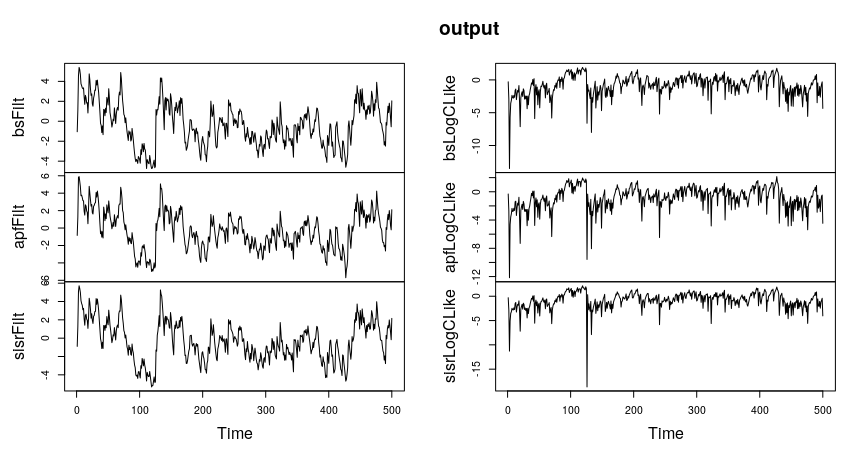
Finally, some time series data is read in, and stored in a \codestd::vector of \codeEigen vectors. The \codestd::vector of lambda functions is provided as a second argument to each particle filter’s \codefilter method. The provided lambda function is called on each particle/sample, and at each time point, the weighted average of all these numbers is returned as an approximation to the filtering expectation The for loop iterates over the data, and at each time point, prints out each model’s estimate of the scalar-valued quantity would correspond with a real-time estimate of the current volatility level for this financial instrument, as well as an estimate for the logarithm of the conditional likelihood .
std::vector<osv> data = readInData<FLOATTYPE,dimobs>(csv); auto idtyLambda = [](const ssv xt) -> const Mat return xt; ; std::vector<std::function<const Mat(const ssv)>> v; v.push_back(idtyLambda); for(size_t row = 0; row < data.size(); ++row) bssvol.filter(data[row], v); apfsvol.filter(data[row], v); sisrsvol.filter(data[row], v);
std::cout << bssvol.getExpectations()[0] << ", " << bssvol.getLogCondLike() << ", " << apfsvol.getExpectations()[0] << ", " << apfsvol.getLogCondLike() << ", " << sisrsvol.getExpectations()[0] << ", " << sisrsvol.getLogCondLike() << "\n";
The above code is built and run with the following commands. It writes all output to a file named \code /Desktop/sample_output.txt. Here we are using the utility \proglangmake. This code was run on the Bourne Again Shell in Ubuntu 18.0.4, but it will likely work on other Mac and Linux machines. If it does not, there might be some small adjustments that need to be made to the file \codeexamples/Makefile–for example, this file assumes the \codeEigen headers are located at \code/usr/include/eigen3. {Code} cd /pf/examples/ make clean make ./examples 1 data/svol_y_data.csv > /Desktop/sample_output.txt
The output can then be more closely evaluated. For example, the following \proglangR code would produce a comparison of the three particle filter’s outputs: {Code} output <- read.csv(" /Desktop/sample_output.txt", header=F) colnames(output) <- c("bsFilt", "apfFilt", "sisrFilt", "bsLogCLike", "apfLogCLike", "sisrLogCLike") plot.ts(output, plot.type = "multiple", nc = 2) This plot is displayed in Figure 2.
4 Summary and discussion
This article has outlined the design of, and provided a fully-worked example for, the \pkgPF library, a \proglangC++ header-only template library for particle filtering. This library will continue to be developed into the foreseeable future, so feature requests and bug reports can be provided after visiting https://github.com/tbrown122387/pf/issues.
Computational details
The results in this paper were obtained with the \pkgPF 1.0.1 library, using the \codegcc 7.4.0 compiler on the \codeUbuntu 18.04 operating system. Compilation of the \codeexamples program was also successfully completed with the \codeclang++-6.0 compiler, as well.
References
- Andrieu and Doucet (2002) Andrieu C, Doucet A (2002). “Particle filtering for partially observed Gaussian state space models.” Journal of the Royal Statistical Society: Series B (Statistical Methodology), 64(4), 827–836. ISSN 1467-9868. 10.1111/1467-9868.00363. URL http://dx.doi.org/10.1111/1467-9868.00363.
- Andrieu et al. (2010) Andrieu C, Doucet A, Holenstein R (2010). “Particle Markov Chain Monte Carlo Methods.” Journal of the Royal Statistical Society: Series B (Statistical Methodology), 72(3), 269–342. ISSN 1467-9868. 10.1111/j.1467-9868.2009.00736.x. URL http://dx.doi.org/10.1111/j.1467-9868.2009.00736.x.
- Baum and Petrie (1966) Baum LE, Petrie T (1966). “Statistical Inference for Probabilistic Functions of Finite State Markov Chains.” Ann. Math. Statist., 37(6), 1554–1563. 10.1214/aoms/1177699147. URL https://doi.org/10.1214/aoms/1177699147.
- Blake and Isard (1997) Blake A, Isard M (1997). “The CONDENSATION algorithm-conditional density propagation and applications to visual tracking.” In Advances in Neural Information Processing Systems, pp. 361–367.
- Bolic et al. (2005) Bolic M, Djuric PM, Sangjin Hong (2005). “Resampling algorithms and architectures for distributed particle filters.” IEEE Transactions on Signal Processing, 53(7), 2442–2450. ISSN 1941-0476. 10.1109/TSP.2005.849185.
- Cappé et al. (2005) Cappé O, Moulines E, Ryden T (2005). Inference in Hidden Markov Models (Springer Series in Statistics). Springer-Verlag, Berlin, Heidelberg. ISBN 0387402640.
- Chen and Liu (2000) Chen R, Liu JS (2000). “Mixture Kalman Filters.” J. R. Statist. Soc. B, 62, 493–508.
- de Valpine et al. (2017) de Valpine P, Turek D, Paciorek CJ, Anderson-Bergman C, Lang DT, Bodik R (2017). “Programming With Models: Writing Statistical Algorithms for General Model Structures With \pkgNIMBLE.” Journal of Computational and Graphical Statistics, 26(2), 403–413. 10.1080/10618600.2016.1172487. https://doi.org/10.1080/10618600.2016.1172487, URL https://doi.org/10.1080/10618600.2016.1172487.
- Del Moral (2004) Del Moral P (2004). Feynman-Kac Formulae: Genealogical and Interacting Particle Systems With Applications, volume 100. ISBN 0387202684. 10.1007/978-1-4684-9393-1.
- Doucet and Johansen (2011) Doucet A, Johansen AM (2011). “A Tutorial on Particle Filtering and Smoothing: Fifteen Years Later.”
- Gordon et al. (1993) Gordon N, Salmond D, Smith A (1993). “Novel approach to nonlinear/non-Gaussian Bayesian state estimation.” IEEE Proceedings F, Radar and Signal Processing, 140(2), 107–113. 10.1049/ip-f-2.1993.0015.
- Guennebaud et al. (2010) Guennebaud G, Jacob B, et al. (2010). “\pkgEigen v3.” http://eigen.tuxfamily.org.
- Hastings (1970) Hastings WK (1970). “Monte Carlo Sampling Methods Using Markov Chains and Their Applications.” Biometrika, 57(1), 97–109. ISSN 00063444. URL http://www.jstor.org/stable/2334940.
- ISO (2012) ISO (2012). ISO/IEC 14882:2011 Information technology — Programming languages — C++. International Organization for Standardization, Geneva, Switzerland. URL http://www.iso.org/iso/iso_catalogue/catalogue_tc/catalogue_detail.htm?csnumber=50372.
- Johansen (2009) Johansen AM (2009). “SMCTC: Sequential Monte Carlo in \proglangC++.” Journal of Statistical Software, 30(6), 1–41. ISSN 1548-7660. URL http://www.jstatsoft.org/v30/i06.
- Kalman (1960) Kalman RE (1960). “A New Approach to Linear Filtering and Prediction Problems.” Transactions of the ASME–Journal of Basic Engineering, 82(Series D), 35–45.
- Kantas et al. (2014) Kantas N, Doucet A, Singh SS, Maciejowski J, Chopin N (2014). “On Particle Methods for Parameter Estimation in State-Space Models.” ArXiv e-prints. 1412.8695.
- Metropolis et al. (1953) Metropolis N, Rosenbluth AW, Rosenbluth MN, Teller AH, Teller E (1953). “Equation of State Calculations by Fast Computing Machines.” The Journal of Chemical Physics, 21(6), 1087–1092. 10.1063/1.1699114. URL http://link.aip.org/link/?JCP/21/1087/1.
- Murray (2013) Murray LM (2013). “Bayesian State-Space Modelling on High-Performance Hardware Using \pkgLibBi.” arXiv:1306.3277.
- Pitt and Shephard (1999) Pitt MK, Shephard N (1999). “Filtering via Simulation: Auxiliary Particle Filters.” 94(446), 590–?? ISSN 0162-1459 (print), 1537-274X (electronic).
- Rabiner (1989) Rabiner LR (1989). “A Tutorial on Hidden Markov Models and Selected Applications in Speech Recognition.” Proceedings of the IEEE, 77(2), 257–286. ISSN 1558-2256. 10.1109/5.18626.
- Shumway and Stoffer (2006) Shumway RH, Stoffer DS (2006). Time Series Analysis and its Applications : With R Examples. Springer texts in statistics. Springer, New York. ISBN 0-387-29317-5. URL http://opac.inria.fr/record=b1122302.
- Taylor (1982) Taylor S (1982). “Financial Returns Modelled by the Product of Two Stochastic Processes, a Study of Daily Sugar Prices 1961-79.” 1.
- Todeschini et al. (2014) Todeschini A, Caron F, Fuentes M, Legrand P, Del Moral P (2014). “\pkgBiips: Software for Bayesian Inference with Interacting Particle Systems.” arXiv preprint arXiv:1412.3779.
- Whiteley et al. (2013) Whiteley N, Lee A, Heine K (2013). “On the role of interaction in sequential Monte Carlo algorithms.” 10.3150/14-BEJ666. arXiv:1309.2918.