A partially overdetermined problem in domains with partial umbilical boundary in space formsThanks: This work is supported by NSFC (Grant No. 11871406).

Jinyu Guo Address: School of Mathematical Sciences
Xiamen University
361005, Xiamen, P.R. China Email address: guojinyu14@163.com and Chao Xia Address: School of Mathematical Sciences
Xiamen University
361005, Xiamen, P.R. China Email address: chaoxia@xmu.edu.cn

Abstract.

In the first part of this paper, we consider a partially overdetermined mixed boundary value problem in space forms and generalize the main result in [11] into the case of general domains with partial umbilical boundary in space forms. Precisely, we prove that a partially overdetermined problem in a domain with partial umbilical boundary admits a solution if and only if the rest part of the boundary is also part of an umbilical hypersurface. In the second part of this paper, we prove a Heintze-Karcher-Ros type inequality for embedded hypersurfaces with free boundary lying on a horosphere or an equidistant hypersurface in the hyperbolic space. As an application, we show Alexandrov type theorem for constant mean curvature hypersurfaces with free boundary in these settings.

1. Introduction

In a celebrated paper [26], Serrin initiated the study of the following overdetermined boundary value problem (BVP)

(1.1)

\begin{cases}{}\Delta u=1,&\text{in}\ \Omega\\ u=0,&\text{on}\ \partial\Omega\\ \partial_{\nu}u=c,&\text{on}\ \partial\Omega,\\ \end{cases}

where $\Omega$ is an open, connected, bounded domain in $\mathbb{R}^{n}$ with smooth boundary $\partial\Omega$ , $c\in\mathbb{R}$ is a constant and $\nu$ is the unit outward normal to $\partial\Omega$ . Serrin proved that if (1.1) admits a solution, then $\Omega$ must be a ball and the solution $u$ is radially symmetric. Serrin’s proof is based on the moving plane method or Alexandrov reflection method, which has been invented by Alexandrov in order to prove the famous nowadays so-called Alexandrov’s soap bubble theorem [1]: any closed, embedded hypersurface of constant mean curvature (CMC) must be a round sphere.

In space forms¹¹ 1 Throughout this paper, we regard an open hemi-sphere as a spherical space form., Serrin’s symmetry result was proved in [13] and [18] by the method of moving plane. A special overdetermined problem in space forms has been considered by Qiu-Xia [21] by using Weinberger’s approach, see also [7]. We also mention that a corresponding result in the closed sphere case is no longer true, see e.g. [8].

Serrin’s overdetermined BVP has close relationship with closed CMC hypersurfaces. Analog to closed CMC hypersurfaces, there are several rigidity results for free boundary CMC hypersurfaces in the Euclidean unit ball $\mathbb{B}^{n}$ . Here we use “free boundary” to mean a hypersurface which intersects $\mathbb{S}^{n-1}$ orthogonally. We refer to a recent survey paper [28] for details. In particular, Alexandrov type theorem says that a free boundary CMC hypersurface in a half ball must be a free boundary spherical cap. Motivated by this, we have proposed in [11] the study of a partially overdetemined BVP in a half ball. Precisely, let $\mathbb{B}^{n}_{+}=\{x\in\mathbb{B}^{n}:x_{n}>0\}$ be the half Euclidean unit ball and $\Omega\subset\mathbb{B}^{n}_{+}$ be an open bounded, connected domain with boundary $\partial\Omega=\bar{\Sigma}\cup T$ , where ${\Sigma}\subset\mathbb{B}^{n}_{+}$ is a smooth open hypersurface and $T\subset\mathbb{S}^{n-1}$ meets ${\Sigma}$ at a common $(n-2)$ -dimensional submanifold $\Gamma\subset\mathbb{S}^{n-1}$ . We have considered the following partially overdetemined BVP in $\Omega$ :

(1.2)

\begin{cases}{}\Delta u=1,&\text{in}\ \Omega\subset\mathbb{B}^{n}_{+},\\ u=0,&\text{on}\ \bar{\Sigma},\\ \partial_{\nu}u=c,&\text{on}\ \bar{\Sigma},\\ \partial_{\bar{N}}u=u,&\text{on}\ T,\end{cases}

where $\nu$ and $\bar{N}(x)=x$ are the outward unit normal of $\Sigma$ and $T\subset\mathbb{S}^{n-1}$ respectively. We have proved the following result.

Theorem 1.1 ([11]).

Let $\Omega$ be as above. Assume (1.2) admits a weak solution

u\in W_{0}^{1,2}(\Omega,{\Sigma})=\{u\in W^{1,2}(\Omega),u|_{\bar{\Sigma}}=0\},

i.e.,

(1.3)

\displaystyle\int_{\Omega}(\langle\nabla u,\nabla v\rangle+v)\,dx-\int_{T}uv\,dA=0,\hbox{ for all }v\in W_{0}^{1,2}(\Omega,{\Sigma}).

Assume further that $u\in W^{1,\infty}(\Omega)\cap W^{2,2}(\Omega).$ Then $\Omega$ must be of the form

(1.4)

\displaystyle\Omega_{nc}(a):=\left\{x\in\mathbb{B}^{n}_{+}:|x-a\sqrt{1+(nc)^{2}}|^{2}<(nc)^{2}\right\},\quad a\in\mathbb{S}^{n-1}

for some $a\in\mathbb{S}^{n-1}$ and

(1.5)

\displaystyle u(x)=u_{a,nc}(x):=\frac{1}{2n}(|x-a\sqrt{1+(nc)^{2}}|^{2}-(nc)^{2}).

We remark that $\partial\Omega_{nc}(a)\cap\mathbb{B}^{n}_{+}$ is a free boundary spherical cap. Thus Theorem 1.1 gives a characterization of free boundary spherical caps by an overdetermined BVP, which can be regarded as Serrin’s analog for the setting of free boundary CMC hypersurfaces in a ball.

In this paper, we will generalize Theorem 1.1 into the setting of domains with partial umbilical boundary in space forms.

Let $(\mathbb{M}^{n}(K),\bar{g})$ be a complete simply-connected Riemann manifold with constant sectional curvature $K$ . Up to homoteties we may assume $K=0,1,-1$ ; the case $K=0$ corresponds to the case of the Euclidean space $\mathbb{R}^{n}$ , $K=1$ is the unit sphere $\mathbb{S}^{n}$ with the round metric and $K=-1$ is the hyperbolic space $\mathbb{H}^{n}$ . We recall some basic facts about umbilical hypersurfaces in $\mathbb{M}^{n}(K)$ . It is well-known that an umbilical hypersuface in space forms has constant principal curvature $\kappa\in\mathbb{R}$ . By a choice of orientation (or normal vector field $\bar{N}$ ), we may assume $\kappa\in[0,\infty)$ . It is also a well-known fact that in $\mathbb{R}^{n}$ and $\mathbb{S}^{n}$ , geodesic spheres $(\kappa>0)$ and totally geodesic hyperplanes $(\kappa=0)$ are all complete umbilical hypersurfaces, while in $\mathbb{H}^{n}$ the family of all complete umbilical hypersurfaces includes geodesic spheres $(\kappa>1)$ , totally geodesic hyperplanes $(\kappa=0)$ , horospheres $(\kappa=1)$ and equidistant hypersurfaces $(0<\kappa<1)$ (see e.g.[16]). We remark that unlike geodesic spheres, the horospheres and the equidistant hypersurfaces are non-compact umbilical hypersurfaces.

We use $S_{K,\kappa}$ to denote an umbilical hypersurface in $\mathbb{M}^{n}(K)$ with principal curvature $\kappa$ . $S_{K,\kappa}$ divides $\mathbb{M}^{n}(K)$ into two connected components. We use $B^{{\rm int}}_{K,\kappa}$ to denote the one component whose outward normal is given by the orientation $\bar{N}$ . The other one we denote by $B^{{\rm ext}}_{K,\kappa}$ . Let $\Omega\subset B^{{\rm int}}_{K,\kappa}$ be a bounded, connected open domain whose boundary $\partial\Omega=\bar{\Sigma}\cup T$ , where ${\Sigma}\subset B^{\rm int}_{K,\kappa}$ is smooth open hypersurface and $T\subset S_{K,\kappa}$ meets $\Sigma$ at a common $(n-2)$ -dimensional submanifold $\Gamma$ . We refer to Figure 1-3 in Section 2 for the corresponding domains for $K=-1$ (hyperbolic space) and different values $\kappa$ .

Since the Euclidean case $K=0$ has already been handled in [11], and the case $\kappa=0$ in $\mathbb{M}^{n}(K)$ has been considered in [6] (as a special case of a flat cone), in this paper we consider the hyperbolic case $K=-1$ with $\kappa>0$ and the spherical case $K=1$ with $\kappa>0$ .

We consider the following mixed BVP in $\Omega\subset B^{\rm int}_{K,\kappa}$ :

(1.6)

\begin{cases}{}\bar{\Delta}u+nKu=1,&\text{in}\ \Omega,\\ u=0,&\text{on}\ \bar{\Sigma},\\ \partial_{\bar{N}}u=\kappa u,&\text{on}\ T.\end{cases}

As we described above, $\bar{N}$ is the unit outward normal of $B^{\rm int}_{K,\kappa}$ .

If $\kappa>0$ , for a general domain, there might not exist a solution to (1.6). Also, for a general domain, the maximum principle fails to hold. These are due to the fact that the Robin boundary condition on $T$ has an unfavorable sign. In our case, we can show that there always exists a unique non-positive solution $u\in C^{\infty}(\bar{\Omega}\setminus\Gamma)\cap C^{\alpha}(\bar{\Omega})$ to (1.6) for some $\alpha\in(0,1)$ , see Proposition 3.3 below.

Remark 1.1.

For the other case ${\Omega}\subseteq{B}^{\rm ext}_{K,\kappa}$ , $-\bar{N}$ plays the role of the unit outward normal of $B^{\rm ext}_{K,\kappa}$ along $T$ . Hence the Robin boundary condition becomes $\partial_{(-\bar{N})}u=-\kappa u$ on $T$ , which has a good sign, i.e. $-\kappa<0$ , according to the classical elliptic PDE theory. The existence of weak solution (1.6) follows directly from the Fredholm alternative theorem (see for example [9]).

In this paper, we study the following partially overdetermined BVP in $\Omega\subset B^{{\rm int}}_{K,\kappa}\quad(B^{{\rm ext}}_{K,\kappa}\hbox{ resp.})$ :

(1.7)

\begin{cases}{}\bar{\Delta}u+nKu=1,&\text{in}\ \Omega,\\ u=0,&\text{on}\ \bar{\Sigma},\\ \partial_{\nu}u=c,&\text{on}\ \bar{\Sigma},\\ \partial_{\bar{N}}u=\kappa u,&\text{on}\ T.\end{cases}

where $\nu$ is the outward unit normal of ${\Sigma}$ . Our main result is the following

Theorem 1.2.

Let $\Omega\subset B^{{\rm int}}_{K,\kappa}\quad(B^{{\rm ext}}_{K,\kappa}\hbox{ resp.})$ . Assume the partially overdetermined BVP (1.7) admits a weak solution $u\in W_{0}^{1,2}(\Omega,{\Sigma})$ , i.e.,

(1.8)

\displaystyle\int_{\Omega}\left(\bar{g}(\bar{\nabla}u,\bar{\nabla}v)+v-nKuv\right)dx-\kappa\int_{T}uv\,dA=0,\hbox{ for all }v\in W_{0}^{1,2}(\Omega,{\Sigma})

together with an additional boundary condition $\partial_{\nu}u=c$ on ${\Sigma}$ . Assume further that

(1.9)

\displaystyle u\in W^{1,\infty}(\Omega)\cap W^{2,2}(\Omega).

(i)

If $S_{K,\kappa}$ is a horosphere $(K=-1$ and $\kappa=1)$ or an equidistant hypersurface $(K=-1$ and $0<\kappa<1)$ in $\mathbb{H}^{n}$ , then $\Sigma$ must be part of an umbilical hypersurface with principal curvature $1/(nc)$ which intersects $S_{K,\kappa}$ orthogonally.
(ii)

If $S_{K,\kappa}$ is a geodesic sphere in $\mathbb{H}^{n}$ or $\mathbb{S}^{n}_{+}$ , that is $K=-1$ and $\kappa>1$ or $K=1$ and $\kappa>0$ , then the same conclusion in (i) holds provided $\Omega\subset B^{{\rm int},+}_{K,\kappa}\quad(B^{{\rm ext},+}_{K,\kappa}\hbox{ resp.})$ .

Here $B^{{\rm int},+}_{K,\kappa}$ means a half ball, see (2.3) below.

Remark 1.2.

The above umbilical hypersurface could be a horosphere, an equidistant hypersurface or a geodesic ball. We will give an example in Appendix A that $\Sigma$ and $T$ are part of two orthogonal horospheres, for which the partially overdetermined BVP (1.7) still admits a solution.

We remark that we do not assume ${\Sigma}$ meets $S_{K,\kappa}$ orthogonally a priori. Thus it is impossible to use the Alexandrov reflection method as Ros-Souam [25]. On the other hand, since the lack of regularity of $u$ on $\Gamma$ , it is difficult to use the maximum principle as Weinberger’s [29]. Higher order regularity up to the interface $\Gamma=\bar{\Sigma}\cap\bar{T}$ is a subtle issue for mixed boundary value problems. A regularity result by Lieberman [15] shows that a weak solution $u$ to (1.7) belongs to $C^{\infty}(\bar{\Omega}\setminus\Gamma)\cap C^{\alpha}(\bar{\Omega})$ for some $\alpha\in(0,1)$ . The regularity assumption (1.9) is for technical reasons, that is, we will use an integration method which requires (1.9) to perform integration by parts.

Similar to the Euclidean case [11], we use a purely integral method to prove our theorem. The integration makes use of a non-negative weight function $V$ , which is given by a multiplier of the divergence of a conformal Killing vector field $X$ . In the case of geodesic spheres in $\mathbb{H}^{n}$ or $\mathbb{S}^{n}_{+}$ , we use $X$ defined by (2.5), which was found in [27]. In the case of horospheres or equidistant hypersurfaces in $\mathbb{H}^{n}$ , we use $X$ defined by (2.6). The common feature of such conformal Killing vector fields is that it is parallel to the support hypersurfaces.

By using $X$ , we get a Pohozaev-type identity with weight $V$ , Proposition 4.3. Then with the usual $P$ -function $P=|\bar{\nabla}u|^{2}-\frac{2}{n}u+Ku^{2}$ , we can show the identity

\int_{\Omega}Vu\big|(\bar{\nabla}^{2}u+Kug)-\frac{1}{n}(\bar{\Delta}u+nKu)\bar{g}\big|^{2}dx=0.

Theorem 1.2 follows since the $P$ -function is subharmonic.

In the second part of this paper, we will use the solution to (1.6) to study Alexandrov type theorem for embedded free boundary CMC hypersurfaces in $\mathbb{H}^{n}$ supported on a horosphere or an equidistant hypersurface.

It is nowadays a routine argument to combine a Minkowski type formula and a sharp Heintze-Karcher-Ros type inequality to prove Alexandrov type theorem, see e.g. [14, 22, 24, 27]. In the spirit of Wang-Xia [27], we shall first use the solution to (1.6) to prove the following Heintze-Karcher-Ros type inequality for free boundary hypersurfaces in $\mathbb{H}^{n}$ supported on a horosphere or an equidistant hypersurface. The case of geodesic hyperplane in space forms has been proved by Pyo, see [20, Theorem 4 and Theorem 10]. The case of geodesic spheres in space forms has been shown by Wang-Xia, see [27, Theorem 5.2 and Theorem 5.4].

Theorem 1.3.

Let $\mathbb{H}^{n}$ be given by the half space model $\{x\in\mathbb{R}^{n}_{+}:x_{n}>0\}$ with hyperbolic metric $\bar{g}=\frac{1}{x_{n}^{2}}\delta$ . Let ${\Sigma}\subset\mathbb{H}^{n}$ be an embedded smooth hypersurface whose boundary $\partial{\Sigma}$ lies on a support hypersurface $S$ (that is, a horosphere or an equidistant hypersurface). Assume ${\Sigma}$ intersects $S$ orthogonally. Assume ${\Sigma}$ has positive normalized mean curvature $H_{1}$ and let $\Omega$ be the enclosed domain by ${\Sigma}$ and $S$ . Then

(1.10)

\displaystyle\int_{{\Sigma}}\frac{1}{x_{n}\cdot H_{1}}dA\geq\int_{\Omega}\frac{n}{x_{n}}dx.

Moreover, the above equality (1.10) holds if and only if ${\Sigma}$ is part of an umbilical hypersurface which meets $S$ orthogonally.

Using the above Heintze-Karcher-Ros type inequality, we are able to reprove Alexandrov type theorem for free boundary constant mean curvature or constant higher order mean curvature hypersurfaces in $\mathbb{H}^{n}$ supported by horospheres and equidistant hypersurfaces, see Theorem 5.2.

We remark that the Alexandrov type theorem in this setting has been shown by [16], using the classical Alexandrov’s reflection method, see also [30]. They were also able to handle in [16] the general capillary hypersurfaces, that is, constant mean curvature hypersurfaces with contstant contact angle.

The rest of the paper is organized as follows. In Section 2, we review the conformal Killing vector fields $X$ we shall use in each case and their properties. In Section 3, we study two kinds of eigenvalue problems in $\Omega$ in space forms and use them to prove the existence and uniqueness of the mixed BVP (1.6). In Section 4, we prove a weighted Pohozaev inequality and then Theorem 1.2. In Section 5, We prove Theorem 1.3 and the Alexandrov type Theorem 5.2.

2. Conformal Killing vector fields in space forms

We first introduce the notations. Let us recall that $S_{K,\kappa}$ is an umbilical hypersurface in $\mathbb{M}^{n}(K)$ with principal curvature $\kappa\in[0,\infty)$ .

2.1. Hyperbolic space $\mathbb{H}^{n}$

Definition 2.1 ([16]).

In hyperbolic space $\mathbb{H}^{n}$ , we call a support hypersurface a complete non-compact umbilical hypersurface, which means geodesic hyperplanes ( $\kappa=0$ ), horospheres ( $\kappa=1$ ) and equidistant hypersurfaces ( $0<\kappa<1$ ).

A horosphere is a ”sphere” whose centre lies at $\partial_{\infty}\mathbb{H}^{n}$ . In the upper half-space model

(2.1)

\displaystyle\mathbb{H}^{n}=\{x=(x_{1},x_{2},\cdots,x_{n})\in\mathbb{R}^{n}_{+}:x_{n}>0\},\quad\bar{g}=\frac{1}{x_{n}^{2}}\delta,

a horosphere, up to a hyperbolic isometry, is given by the horizontal plane

L(1)=\{x\in\mathbb{R}^{n}_{+}:x_{n}=1\}

By choosing $\bar{N}=-E_{n}=(0,\cdots,0,-1)$ , the principal curvature of a horosphere is given by $\kappa=1$ . We remark that a horosphere is isometric to a Euclidean plane.

An equidistant hypersurface is a connected component of the set of points equidistant from a given hyperplane. In the half-space model, an equidistant hypersurface, is given by a sloping Euclidean hyperplane $\Pi$ which meets $\partial_{\infty}\mathbb{H}^{n}$ with angle $\theta$ through a point $E_{n}=(0,0,\cdots,1)\in\mathbb{R}^{n}_{+}$ , say

\Pi=\{x\in\mathbb{R}^{n}_{+}:x_{1}\tan\theta+x_{n}=1\}

and by choosing $\bar{N}$ as the same direction as $(-\tan\theta,0,\cdots,0,-1)$ , it’s principal curvature is $\kappa=\cos\theta\in(0,1)$ .

Next we clarify the unified notation we will use in each case.

•

Case 1. If $S_{K,\kappa}$ is a geodesic sphere of radius $R$ , then $\kappa=\coth R\in(1,\infty)$ and let $B_{K,\kappa}^{\rm int}$ denote the geodesic ball enclosed by $S_{K,\kappa}$ . By using the poincare ball model

(2.2) $\displaystyle\mathbb{B}^{n}=\{x\in\mathbb{R}^{n}:|x|<1\},\quad\bar{g}=\frac{4}{(1-|x|^{2})^{2}}\delta,$

we have up to an hyperbolic isometry,

$B_{K,\kappa}^{\rm int}=\left\{x\in\mathbb{B}^{n}:|x|\leq R_{\mathbb{R}}:=\sqrt{\frac{1-\arccosh R}{1+\arccosh R}}\right\}.$

Moreover, we let

(2.3) $\displaystyle B^{{\rm int},+}_{K,\kappa}=\left\{x\in B_{K,\kappa}^{\rm int}:x_{n}>0\right\}$

be a geodesic half ball. See Figure 1.

•

Case 2. If $S_{K,\kappa}$ is a support hypersurface, then $\kappa\in[0,1]$ . By using the upper half-space model (2.1), we have, up to an hyperbolic isometry,

(2.4)

B_{K,\kappa}^{\rm int}=\begin{cases}{}\{x\in\mathbb{R}^{n}_{+}:x_{n}>1\},&\text{if}\,\,\kappa=1,\\ \{x\in\mathbb{R}^{n}_{+}:x_{1}\tan\theta+x_{n}>1\},&\text{if}\,\,\kappa=\cos\theta\in(0,1).\\ \end{cases}

See Figure 2 and 3.

Refer to caption — Figure 1. $S_{K,\kappa}$ is a geodesic sphere with principal curvature $\kappa=\coth R>1$ and the shaded area is $B_{K,\kappa}^{\rm int,+}$

Next we introduce the conformal Killing vector field $X$ in $\mathbb{H}^{n}$ and the weight $V$ we will use later.

•

Case 1. $\kappa>1$ . In this case, as before we use the Poincaré ball model (2.2). Denote

(2.5) $X:=\frac{2}{1-R_{\mathbb{R}}^{2}}[x_{n}x-\frac{1}{2}(|x|^{2}+R_{\mathbb{R}}^{2})E_{n}],\quad V=\frac{2x_{n}}{1-|x|^{2}}.$
•

Case 2. $0<\kappa\leq 1$ . In this case, as before we use the upper half-space model (2.1). Denote

(2.6) $X:=x-E_{n},\quad V=\frac{1}{x_{n}}.$

Proposition 2.1.

$(i)$ $X$ is a conformal Killing vector field with $L_{X}\bar{g}=V\bar{g}$ , namely

(2.7)

\displaystyle\frac{1}{2}(\bar{\nabla}_{i}X_{j}+\bar{\nabla}_{j}X_{i})=V\bar{g}_{ij}.

(ii)

$X\mid_{S_{K,\kappa}}$ is a tangential vector field on $S_{K,\kappa}$ , i.e.,

(2.8) $\displaystyle\bar{g}(X,\bar{N})=0\,\,\text{\rm on}\,\,S_{K,\kappa}.$

Proof.

Case 1. $\kappa>1$ , see [27, Proposition 4.1].

Case 2. $0<\kappa\leq 1$ , we choose an orthonormal basis $\{e_{i}\}_{i=1}^{n}$ in the upper half-space model,

e_{i}=x_{n}E_{i},\quad i=1,\cdots,n.

where $\{E_{i}\}_{i=1}^{n}$ is the Euclidean orthonormal basis in $\mathbb{R}^{n}$ . Then

(2.9)		$\displaystyle\frac{1}{2}(\bar{\nabla}_{i}X_{j}+\bar{\nabla}_{j}X_{i})$	$\displaystyle=$	$\displaystyle\frac{1}{2}(D_{i}X_{j}+D_{j}X_{i})+X(-\ln x_{n})\bar{g}_{ij}$
(2.9)			$\displaystyle=$	$\displaystyle\bar{g}_{ij}+(\frac{1}{x_{n}}-1)\bar{g}_{ij}=\frac{1}{x_{n}}\bar{g}_{ij},$

where $D$ is the Levi-Civita connection in $\mathbb{R}^{n}$ . We use the relationship of $\bar{\nabla}$ and $D$ , that is,

(2.10)

\bar{\nabla}_{Y}Z=D_{Y}Z+Y(-\ln x_{n})Z+Z(-\ln x_{n})Y-\langle Y,Z\rangle D(-\ln x_{n}).

Here $\langle\cdot,\cdot\rangle$ is the Euclidean inner product.

On the other hand,

(2.11)

\displaystyle\bar{g}(X,\bar{N})=\frac{1}{x_{n}}\langle x-E_{n},N_{\delta}\rangle=0\quad\text{on}\,\,S_{K,\kappa}

where $N_{\delta}$ is outward normal to support hypersurface with respect to the Euclidean metric $\delta$ . ∎

Proposition 2.2.

$V$ satisfies the following properties:

(2.12)

\bar{\nabla}^{2}V=-KV\bar{g},

(2.13)

\partial_{\bar{N}}V=\kappa V\quad\,\,\text{on}\,\,S_{K,\kappa},

where $\bar{N}$ is the outward unit normal of $B_{K,\kappa}^{\rm int}$ .

Proof.

Case 1. $\kappa>1$ , see [27, Proposition 4.2].

Case 2. $0<\kappa\leq 1$ . For (2.12), we take normal coordinates $\{e_{i}\}_{i=1}^{n}$ at $p$ such that $\bar{\nabla}_{e_{i}}e_{j}\mid_{p}=0$ . Then

(2.14)		$\displaystyle\bar{\nabla}_{e_{i}}\bar{\nabla}_{e_{j}}V$	$\displaystyle=$	$\displaystyle\bar{\nabla}_{e_{i}}\bar{\nabla}_{e_{j}}(\frac{1}{x_{n}})=\bar{\nabla}_{e_{i}}\left(\bar{\nabla}_{e_{j}}(\frac{1}{x_{n}})\right)=-e_{i}\left(\bar{g}(E_{n},e_{j})\right)$
(2.14)			$\displaystyle=$	$\displaystyle-\bar{g}(\bar{\nabla}_{e_{i}}E_{n},e_{j})=E_{n}(\ln x_{n})\bar{g}_{ij}=\frac{1}{x_{n}}\bar{g}_{ij},$

where we use formula (2.10).

For (2.13), we compute

(2.15)

\displaystyle\partial_{\bar{N}}V=\partial_{\bar{N}}(\frac{1}{x_{n}})=-\frac{1}{x_{n}^{2}}\langle E_{n},\bar{N}\rangle=-\frac{1}{x_{n}^{2}}\langle E_{n},x_{n}N_{\delta}\rangle=\frac{1}{x_{n}}\cos\theta

Here we use the fact that $\langle E_{n},N_{\delta}\rangle=-\cos\theta$ on the support hypersurface $S_{K,\kappa}$ . ∎

2.2. Spherical space $\mathbb{S}^{n}$

In this subsection, we sketch the necessary modifications in the case that the ambient space is the spherical space $\mathbb{S}^{n}$ . We use the model

\left(\mathbb{R}^{n},\,\bar{g}_{\mathbb{S}}=\frac{4}{(1+|x|^{2})^{2}}\delta\right)

to represent $\mathbb{S}^{n}\setminus\{\mathcal{S}\}$ , the unit sphere without the south pole. Therefore, if $S_{K,\kappa}$ is a geodesic sphere of radius $R$ , then in the above model

S_{K,\kappa}=\left\{x\in\mathbb{R}^{n}:|x|=R_{\mathbb{R}}:=\sqrt{\frac{1-\cos R}{1+\cos R}}\right\}.

Then $\kappa=\cot R>0$ , for $R<\frac{\pi}{2}$ . Let $B^{{\rm int}}_{K,\kappa}$ be a geodesic ball enclosed by $S_{K,\kappa}$ and $B^{{\rm int},+}_{K,\kappa}$ be the geodesic half ball given by

(2.16)

B^{{\rm int},+}_{K,\kappa}=\{x\in B^{{\rm int}}_{K,\kappa}:\,x_{n}>0\}.

Let $X$ be the vector field

(2.17)

X=\frac{2}{1+R_{\mathbb{R}}^{2}}[x_{n}x-\frac{1}{2}(|x|^{2}+R_{\mathbb{R}}^{2})E_{n}],\quad V=\frac{2x_{n}}{1+|x|^{2}}.

It has been shown in [27] that $X$ and $V$ also satisfy Propositions 2.1 and 2.2.

3. Mixed BVP in space forms

From this section on, let $\Omega$ be a bounded, connected open domain in $B^{{\rm int}}_{K,\kappa}$ whose boundary $\partial\Omega$ consists two parts $\bar{\Sigma}$ and $T=\partial\Omega\setminus\bar{\Sigma}$ , where $T\subset S_{K,\kappa}$ is smooth and meets $\Sigma$ at a common $(n-2)$ -dimensional submanifold $\Gamma$ . If $S_{K,\kappa}$ is a geodesic sphere, then we assume further that $\Omega\subset B^{{\rm int},+}_{K,\kappa}$ . For notation simplicity and unification, in the following sections, we use $\Omega\subset B^{{\rm int}}_{K,\kappa}$ to indicate that $\Omega\subset B^{{\rm int},+}_{K,\kappa}$ in the case that $S_{K,\kappa}$ is a geodesic sphere.

We consider the following two kinds of eigenvalue problems in $\Omega$ .
I. Mixed Robin-Dirichlet eigenvalue problem

(3.1)

\begin{cases}{}\bar{\Delta}u=-\lambda u,&\hbox{ in }\Omega,\\ u=0,&\hbox{ on }\bar{\Sigma},\\ \partial_{\bar{N}}u=\kappa u,&\hbox{ on }T.\end{cases}

The first Robin-Dirichlet eigenvalue can be variational characterized by

(3.2)

\displaystyle\lambda_{1}=\inf_{0\neq u\in W_{0}^{1,2}(\Omega,{\Sigma})}\frac{\int_{\Omega}\bar{g}(\bar{\nabla}u,\bar{\nabla}u)dx-\kappa\int_{T}u^{2}dA}{\int_{\Omega}u^{2}dx}.

II. Mixed Steklov-Dirichlet eigenvalue problem. (see e.g. [2, 5])

(3.3)

\begin{cases}{}\bar{\Delta}u+nKu=0,&\hbox{ in }\Omega,\\ u=0,&\hbox{ on }\bar{\Sigma},\\ \partial_{\bar{N}}u=\mu\kappa u,&\hbox{ on }T.\end{cases}

The mixed Steklov-Dirichlet eigenvalues can be considered as the eigenvalues of the Dirichlet-to-Neumann map

	$\displaystyle\mathcal{L}:$	$\displaystyle L^{2}(T)\to$	$\displaystyle L^{2}(T)$
		$\displaystyle u\mapsto$	$\displaystyle\frac{1}{\kappa}\partial_{\bar{N}}\hat{u}$

where $\hat{u}\in W_{0}^{1,2}(\Omega,{\Sigma})$ is the extension of $u$ to $\Omega$ satisfying $\bar{\Delta}\hat{u}+nK\hat{u}=0$ in $\Omega$ and $\hat{u}=0$ on ${\Sigma}$ . According to the spectral theory for compact, symmetric linear operators, $\mathcal{L}$ has a discrete spectrum $\{\mu_{i}\}_{i=1}^{\infty}$ (see e.g. [2] or [5]),

0<\mu_{1}\leq\mu_{2}\leq\cdots\to+\infty.

The first eigenvalue $\mu_{1}$ can be variational characterized by

\displaystyle\mu_{1}=\inf_{0\neq u\in W_{0}^{1,2}(\Omega,{\Sigma})}\frac{\int_{\Omega}\bar{g}(\bar{\nabla}u,\bar{\nabla}u)dx-nK\int_{\Omega}u^{2}dx}{\kappa\int_{T}u^{2}dA}.

In our case, we have

Proposition 3.1.

If $S_{K,\kappa}$ is geodesic sphere in $\mathbb{H}^{n}$ or $\mathbb{S}^{n}$ and $\Omega\subseteq B_{K,\kappa}^{\rm int,+}$ , then

(i)

$\lambda_{1}(\Omega)\geq nK$ and $\lambda_{1}=nK$ if and only if $\Omega=B_{K,\kappa}^{\rm int,+}$ .
(ii)

$\mu_{1}(\Omega)\geq 1$ and $\mu_{1}=1$ if and only if $\Omega=B_{K,\kappa}^{\rm int,+}$ .

Proof.

We proceed exactly as [11]. If $\Omega=B_{K,\kappa}^{\rm int,+}$ , one checks that $u=V\geq 0$ indeed solves (3.1) with $\lambda=nK$ and (3.3) with $\mu=1$ . Since $u=V$ is a non-negative solution, it must be the first eigenfunction and hence $\lambda_{1}(B_{K,\kappa}^{\rm int,+})=nK$ and $\mu_{1}(B_{K,\kappa}^{\rm int,+})=1.$

On the other hand, for $\Omega\subset B_{K,\kappa}^{\rm int,+}$ , by the variational characterization and a standard argument of doing zero extension, one sees $\lambda_{1}(\Omega)\geq\lambda_{1}(B_{K,\kappa}^{\rm int,+})=nK$ and $\mu_{1}(\Omega)\geq\mu_{1}(B_{K,\kappa}^{\rm int,+})=1.$

If $\Omega\subsetneqq B_{K,\kappa}^{\rm int,+}$ , then the Aronszajn unique continuity theorem [3] implies $\lambda_{1}(\Omega)>\lambda_{1}(B_{K,\kappa}^{\rm int,+})=nK$ . In fact, we extend the first Robin-Dirichlet eigenfunction $u$ in $\Omega$ to $\tilde{u}$ in $B_{K,\kappa}^{\rm int,+}$ by defining $\tilde{u}=0$ outside $\bar{\Omega}$ . Then $\tilde{u}$ is the first Robin-Dirichlet eigenfunction in $B_{K,\kappa}^{\rm int,+}$ by its variational characterization (3.2). However, the Aronszajn unique continuity theorem²² 2 Let $\mathcal{L}$ be a second order elliptic operator with $C^{3}$ coefficients. If $\mathcal{L}u=0$ in an open connected domain $\Omega$ and $u=0$ in an open subset of $\Omega$ , then $u=0$ is identically zero in $\Omega$ . would imply that $u=0$ is identically zero on $B_{K,\kappa}^{\rm int,+}$ . This is a contradiction that $u$ is the first eigenfunction in $\Omega$ .

For $\mu_{1}$ , it has been proved in [5, Proposition 3.1.1], that $\mu_{1}(\Omega)>\mu_{1}(B_{K,\kappa}^{\rm int,+})=1$ . ∎

Proposition 3.2.

If $S_{K,\kappa}$ is a horosphere or an equidistant hypersurface in $\mathbb{H}^{n}$ and $\Omega\subseteq B_{K,\kappa}^{\rm int}$ , then

(3.4)

\lambda_{1}(\Omega)>-n\,\,\text{\rm and}\,\,\mu_{1}(\Omega)>1.

Proof.

We first take an orthonormal basis $\{e_{i}\}_{i=1}^{n}$ in the upper half space model

e_{i}=x_{n}E_{i},\quad i=1,\cdots,n.

By using the divergence theorem, we get

(3.5)

\displaystyle\int_{\Omega}{\rm div}_{\bar{g}}(u^{2}e_{n})dx=\int_{\partial\Omega}u^{2}\bar{g}(e_{n},\nu)dA=\int_{T}u^{2}\bar{g}(e_{n},\bar{N})dA=-\cos\theta\int_{T}u^{2}dA

where we also use $u=0$ on $\Sigma$ and the fact $\langle\bar{N},E_{n}\rangle=-x_{n}\cos\theta$ on $T$ and $\theta\in[0,\frac{\pi}{2})$ .

On the other hand,

(3.6)

\int_{\Omega}{\rm div}_{\bar{g}}(u^{2}e_{n})dx=\int_{\Omega}e_{n}(u^{2})dx+\int_{\Omega}u^{2}{\rm div}_{\bar{g}}(e_{n})dx=\int_{\Omega}e_{n}(u^{2})dx-(n-1)\int_{\Omega}u^{2}dx.

Combining (3.5) with (3.6), we have

(3.7)	$\displaystyle\cos\theta\int_{T}u^{2}dA$	$\displaystyle=$	$\displaystyle\int_{\Omega}(n-1)u^{2}-e_{n}(u^{2})dx=\int_{\Omega}(n-1)u^{2}-2ue_{n}(u)dx$
		$\displaystyle\leq$	$\displaystyle\int_{\Omega}(n-1)u^{2}+2\|u\|\|\bar{\nabla}u\|dx$
		$\displaystyle\leq$	$\displaystyle\int_{\Omega}(n-1)u^{2}+\|u\|^{2}+\bar{g}(\bar{\nabla}u,\bar{\nabla}u)dx$
		$\displaystyle=$	$\displaystyle\int_{\Omega}nu^{2}+\bar{g}(\bar{\nabla}u,\bar{\nabla}u)dx$

Since $0\neq u\in W_{0}^{1,2}(\Omega,{\Sigma})$ , we know that the above equality is strict, namely,

(3.8)

\displaystyle\cos\theta\int_{T}u^{2}dA<\int_{\Omega}nu^{2}+\bar{g}(\bar{\nabla}u,\bar{\nabla}u)dx

Recall that $\kappa=\cos\theta$ . Therefore, we complete this proof by taking infimum for $u$ .

∎

Using Proposition 3.1 (ii) and 3.2, we show the existence and uniqueness of mixed BVP (1.6).

Proposition 3.3.

Let $f\in C^{\infty}(\Omega)$ , $q\in C^{\infty}(T)$ and $\Omega\subsetneqq B_{K,\kappa}^{\rm int}$ . Then the mixed BVP

(3.9)

\begin{cases}{}\bar{\Delta}u+nKu=f,&\hbox{ in }\Omega,\\ u=0,&\hbox{ on }\bar{\Sigma},\\ \partial_{\bar{N}}u=\kappa u+q,&\hbox{ on }T.\end{cases}

admits a unique weak solution $u\in W^{1,2}_{0}(\Omega,{\Sigma})$ . Moreover, $u\in C^{\infty}(\bar{\Omega}\setminus\Gamma)\cap C^{\alpha}(\bar{\Omega})$ for some $\alpha\in(0,1)$ .

Proof.

The weak solution to (3.9) is defined to be $u\in W_{0}^{1,2}(\Omega,{\Sigma})$ such that

(3.10)

B[u,v]:=\int_{\Omega}\bar{g}(\bar{\nabla}u,\bar{\nabla}v)dx-\kappa\int_{T}uv\,dA-nK\int_{\Omega}uvdx\hbox{ for all }v\in W_{0}^{1,2}(\Omega,{\Sigma}),

(3.11)

\displaystyle B[u,v]=\int_{\Omega}-fv\,dx+\int_{T}qv\,dA\,\hbox{ for all }v\in W_{0}^{1,2}(\Omega,{\Sigma}).

From Proposition 3.1(ii) and Proposition 3.2, we know $1-\frac{1}{\mu_{1}}>0$ . There holds

(3.12)

\kappa\int_{T}u^{2}dA\leq\frac{1}{\mu_{1}}(\int_{\Omega}\bar{g}(\bar{\nabla}u,\bar{\nabla}u)dx-nK\int_{\Omega}u^{2}dA),

By using (3.10), (3.12) and Proposition 3.1 (i) and 3.2, there exists a positive constant $\beta$ such that

(3.13)

\displaystyle B[u,u]\geq(1-\frac{1}{\mu_{1}})(\int_{\Omega}\bar{g}(\bar{\nabla}u,\bar{\nabla}u)\,dx-nK\int_{\Omega}u^{2}dx)\geq\beta\|u\|^{2}_{W_{0}^{1,2}(\Omega,{\Sigma})}

Thus $B[u,v]$ is coercive on $W_{0}^{1,2}(\Omega,{\Sigma})$ . The standard Lax-Milgram theorem holds for the weak formulation to (3.9). Therefore, (3.9) admits a unique weak solution $u\in W_{0}^{1,2}(\Omega,{\Sigma})$ .

The regularity $u\in C^{\infty}(\bar{\Omega}\setminus\Gamma)$ follows from the classical regularity theory for elliptic equations and $u\in C^{\alpha}(\bar{\Omega})$ has been proved by Lieberman [15, Theorem 2]. Note that the global wedge condition in [15, Theorem 2] is satisfied for the domain $\Omega$ whose boundary parts ${\Sigma}$ and $T$ meet at a common in smooth $(n-2)$ -dimensional manifold, see page 426 of [15]. ∎

Proposition 3.4.

Let $u$ be the unique solution to (3.9) with $f\geq 0$ and $q\leq 0$ . Then either $u\equiv 0$ in $\Omega$ or $u<0$ in $\Omega\cup T$ .

Proof.

Since the Robin boundary condition has an unfavorable sign, we cannot use the maximum principle directly. Since $u_{+}=\text{max}\{u,0\}\in W_{0}^{1,2}(\Omega,{\Sigma})$ , we can use it as a test function in the weak formulation (3.11) to get

\displaystyle\int_{\Omega}-fu_{+}\,dx+\int_{T}qu_{+}\,dA

\displaystyle=\int_{\Omega}\bar{g}(\bar{\nabla}u_{+},\bar{\nabla}u_{+})dx-\kappa\int_{T}(u_{+})^{2}\,dA-nK\int_{\Omega}(u_{+})^{2}dx.

Since $f\geq 0$ and $q\leq 0$ , we have

\displaystyle\int_{\Omega}-fu_{+}\,dx+\int_{T}qu_{+}\,dA\leq 0.

On the other hand, it follows from Proposition 3.1 (i) and (3.4) that

\displaystyle\int_{\Omega}\bar{g}(\bar{\nabla}u_{+},\bar{\nabla}u_{+})dx-\kappa\int_{T}(u_{+})^{2}\,dA-nK\int_{\Omega}(u_{+})^{2}dx\geq(\lambda_{1}-nK)\int_{\Omega}(u_{+})^{2}dx\geq 0.

From above, we conclude that $u_{+}\equiv 0$ , which means $u\leq 0$ in $\Omega$ . Finally, by the strong maximum principle, we get either $u\equiv 0$ in $\Omega$ or $u<0$ in $\Omega\cup T$ . ∎

Proposition 3.5.

Let $e^{T}$ be a tangent vector field to $T$ . Let $u$ be the unique solution to (1.6). Then

(3.14)

\bar{\nabla}^{2}u(\bar{N},e^{T})=0\quad on\ T.

Proof.

By differentiating the equation $\partial_{\bar{N}}u=\kappa u$ with respect to $e^{T}$ , we get

	$\displaystyle\kappa\bar{\nabla}_{e^{T}}(u)$	$\displaystyle={e^{T}}(\bar{g}(\bar{\nabla}u,\bar{N}))=\bar{\nabla}^{2}u(\bar{N},e^{T})+\bar{g}(\bar{\nabla}u,\bar{\nabla}_{e^{T}}\bar{N})$
		$\displaystyle=\bar{\nabla}^{2}u(\bar{N},e^{T})+h^{S_{K,\kappa}}(\bar{\nabla}u,e^{T})=\bar{\nabla}^{2}u(\bar{N},e^{T})+\kappa\bar{g}(\bar{\nabla}u,e^{T}).$

Here we use the fact that $S_{K,\kappa}$ is an umbilical hypersurface with principal curvature $\kappa$ . The assertion (3.14) follows. ∎

4. Partially overdetermined BVP in space forms

In this section we will use a method totally based on integral identities and inequalities to prove Theorem 1.2. The proof follows closely our previous paper [11]. The main ingredient is Propositions 2.1 and 2.2.

First we introduce $P$ function as follows,

(4.1)

P:=\bar{g}(\bar{\nabla}u,\bar{\nabla}u)-\frac{2}{n}u+Ku^{2}.

Proposition 4.1.

$\bar{\Delta}P=2\big|(\bar{\nabla}^{2}u+Kug)-\frac{1}{n}(\bar{\Delta}u+nKu)\bar{g}\big|^{2}\geq 0\hbox{ in }\Omega.$

Proof.

By direct computation and using $\bar{\Delta}u+nKu=1$ ,

	$\displaystyle\bar{\Delta}P(x)$	$\displaystyle=2\|\bar{\nabla}^{2}u\|^{2}+2\bar{g}(\bar{\nabla}u,\bar{\nabla}\bar{\Delta}u)+2\overline{Ric}(\bar{\nabla}u,\bar{\nabla}u)-\frac{2}{n}\bar{\Delta}u+2K(\bar{g}(\bar{\nabla}u,\bar{\nabla}u)+u\bar{\Delta}u)$
		$\displaystyle=2\big\|(\bar{\nabla}^{2}u+Kug)-\frac{1}{n}(\bar{\Delta}u+nKu)\bar{g}\big\|^{2}$
		$\displaystyle\geq 0.$

∎

Due to the lack of regularity, we need the following formula of integration by parts, see [19, Lemma 2.1]. (The original statement [19, Lemma 2.1] is for a sector-like domain in a cone. Nevertheless, the proof is applicable in our case). We remark that a general version of integration-by-parts formula for Lipschitz domains has been stated in some classical book by Grisvard [10, Theorem 1.5.3.1]. However, it seems not enough for our purpose.

Proposition 4.2 ([19], lemma 2.1).

Let $F:\Omega\to\mathbb{R}^{n}$ be a vector field such that

\displaystyle F\in C^{1}(\Omega\cup{\Sigma}\cup T)\cap L^{2}(\Omega)\quad\hbox{ and }\quad{\rm div}(F)\in L^{1}(\Omega).

Then

\displaystyle\int_{\Omega}{\rm div}(F)dx=\int_{{\Sigma}}\bar{g}(F,\nu)dA+\int_{T}\bar{g}(F,\bar{N})dA.

We first prove a Pohozaev-type identity for (1.7).

Proposition 4.3.

Let $u$ be the unique solution to (1.7). Then we have

(4.2)

\int_{\Omega}V(P-c^{2})dx=0.

Proof.

First of all, we remark that by regularity in Proposition 3.3, $u\in C^{\infty}(\Omega\cup{\Sigma}\cup T)$ , that is, $u$ is smooth away from the corner $\Gamma$ . Moreover, due to our assumption $u\in W^{1,\infty}(\Omega)\cap W^{2,2}(\Omega)$ , Proposition 4.2 can be applied in all the following integration by parts.

Now we consider the following differential identity

(4.3)		$\displaystyle{\rm div}(uX-\bar{g}(X,\bar{\nabla}u)\bar{\nabla}u)$
	$\displaystyle=\bar{g}(X,\bar{\nabla}u)+u{\rm div}X-\bar{\nabla}X(\bar{\nabla}u,\bar{\nabla}u)-\frac{1}{2}\bar{g}(X,\bar{\nabla}\bar{g}(\bar{\nabla}u,\bar{\nabla}u))-\bar{g}(X,\bar{\nabla}u)\bar{\Delta}u$
	$\displaystyle=nVu-V\bar{g}(\bar{\nabla}u,\bar{\nabla}u)-\frac{1}{2}\bar{g}(X,\bar{\nabla}\bar{g}(\bar{\nabla}u,\bar{\nabla}u))+nK\bar{g}(X,\bar{\nabla}(\frac{1}{2}u^{2})).$

where we use equation $\bar{\Delta}u+nKu=1$ and (2.7).

Integrating by parts and using (2.8) and boundary conditions (1.7), we see that

(4.4)				$\displaystyle-c^{2}\int_{\Sigma}\bar{g}(X,\nu)dA-\int_{T}\bar{g}(X,\bar{\nabla}u)u_{\bar{N}}dA$
(4.4)			$\displaystyle=$	$\displaystyle\int_{\Omega}\left(nVu-V\bar{g}(\bar{\nabla}u,\bar{\nabla}u)+\frac{1}{2}\bar{g}(\bar{\nabla}u,\bar{\nabla}u){\rm div}X-\frac{nK}{2}u^{2}{\rm div}X\right)dx-\frac{c^{2}}{2}\int_{\Sigma}\bar{g}(X,\nu)dA.$

It follows that

(4.5)		$\displaystyle\int_{\Omega}\left(nVu+(\frac{n}{2}-1)V\bar{g}(\bar{\nabla}u,\bar{\nabla}u)-\frac{n^{2}K}{2}Vu^{2}\right)dx$
	$\displaystyle=-\frac{c^{2}}{2}\int_{\Sigma}\bar{g}(X,\nu)dA-\kappa\int_{T}\bar{g}(X,\bar{\nabla}u)udA.$

Using (2.7) and (2.8) yields

(4.6)		$\displaystyle\int_{\Sigma}\frac{1}{2}c^{2}\bar{g}(X,\nu)dA=\frac{1}{2}c^{2}\left(\int_{\Omega}{\rm div}Xdx-\int_{T}\bar{g}(X,\bar{N})dA\right)=\frac{n}{2}c^{2}\int_{\Omega}Vdx,$
(4.7)		$\displaystyle\kappa\int_{T}\ \bar{g}(X,\bar{\nabla}u)udA=\kappa\int_{T}\bar{g}(X^{T},\bar{\nabla}(\frac{1}{2}u^{2}))dA$
	$\displaystyle\qquad\qquad\qquad\qquad\quad=\frac{\kappa}{2}\int_{\Gamma}u^{2}\bar{g}(X^{T},\mu)ds-\frac{\kappa}{2}\int_{T}u^{2}{\rm div}_{T}X^{T}dA$
	$\displaystyle\qquad\qquad\qquad\qquad\quad=\frac{\kappa(1-n)}{2}\int_{T}Vu^{2}dA.$

In the last equality we also used $u=0$ on $\Gamma$ and ${\rm div}_{T}X^{T}=(n-1)V$ .

To achieve (4.2), we do a further integration by parts and apply (2.12) and (2.13) get

$\displaystyle\int_{\Omega}V\bar{g}(\bar{\nabla}u,\bar{\nabla}u)dx$	$\displaystyle=$	$\displaystyle\int_{T}Vu(u_{\bar{N}})dA-\int_{\Omega}\left(\bar{g}(\bar{\nabla}V,\bar{\nabla}(\frac{1}{2}u^{2}))+Vu\bar{\Delta}u\right)dx$
	$\displaystyle=$	$\displaystyle\kappa\int_{T}Vu^{2}dA-\frac{1}{2}\int_{T}(V)_{\bar{N}}u^{2}dA+\int_{\Omega}(\frac{1}{2}u^{2}\bar{\Delta}V-Vu\bar{\Delta}u)dx$
	$\displaystyle=$	$\displaystyle\kappa\int_{T}Vu^{2}dA-\frac{\kappa}{2}\int_{T}Vu^{2}dA+\int_{\Omega}\frac{1}{2}u^{2}(-nKV)-Vu(1-nKu)dx$
	$\displaystyle=$	$\displaystyle\frac{\kappa}{2}\int_{T}Vu^{2}dA+\frac{nK}{2}\int_{\Omega}Vu^{2}dx-\int_{\Omega}Vudx.$

It follows that

(4.8)

\displaystyle\frac{\kappa}{2}\int_{T}Vu^{2}dA=\int_{\Omega}\left(V\bar{g}(\bar{\nabla}u,\bar{\nabla}u)-\frac{nK}{2}Vu^{2}+Vu\right)dx.

Substituting (4.6)-(4.8) into (4.5), we arrive at (4.2). ∎

Proposition 4.4.

Let $u$ be the unique solution to (1.7) such that $u\in W^{1,\infty}(\Omega)\cap W^{2,2}(\Omega)$ . Then

(4.9)

\displaystyle\int_{\Omega}Vu\big|(\bar{\nabla}^{2}u+Kug)-\frac{1}{n}(\bar{\Delta}u+nKu)\bar{g}\big|^{2}\,dx=0.

Proof.

Since $u\in W^{1,\infty}(\Omega)\cap W^{2,2}(\Omega)$ , then

(4.10)

\displaystyle\Delta P=2\big|(\bar{\nabla}^{2}u+Kug)-\frac{1}{n}(\bar{\Delta}u+nKu)\bar{g}\big|^{2}\in L^{1}(\Omega).

It follows that

{\rm div}(Vu\bar{\nabla}P-P\bar{\nabla}(Vu))\in L^{1}(\Omega)\quad\hbox{ and }\quad(Vu\bar{\nabla}P-P\bar{\nabla}(Vu))\in L^{2}(\Omega).

Firstly, we consider the following differential identity

(4.11)		$\displaystyle{\rm div}(Vu\bar{\nabla}P-P\bar{\nabla}(Vu))+c^{2}{\rm div}(V\bar{\nabla}u-u\bar{\nabla}V)$
	$\displaystyle=$	$\displaystyle Vu\bar{\Delta}P-P\bar{\Delta}(Vu)+c^{2}(V\bar{\Delta}u-u\bar{\Delta}V)$
	$\displaystyle=$	$\displaystyle Vu\bar{\Delta}P-2P\bar{g}(\bar{\nabla}V,\bar{\nabla}u)-(P+c^{2})u\bar{\Delta}V+(c^{2}-P)V\bar{\Delta}u$
	$\displaystyle=$	$\displaystyle Vu\bar{\Delta}P-2P\bar{g}(\bar{\nabla}V,\bar{\nabla}u)-(P+c^{2})u(-nKV)+(c^{2}-P)V(1-nKu)$
	$\displaystyle=$	$\displaystyle Vu\bar{\Delta}P-2P\bar{g}(\bar{\nabla}V,\bar{\nabla}u)+2nKPuV-(P-c^{2})V.$

where we use the fact that $\bar{\nabla}^{2}V=-KV\bar{g}$ and the equation $\bar{\Delta}u+nKu=1$ in $\Omega$ .

Applying divergence theorem in (4.11) and boundary conditions (1.7), we have

(4.12)		$\displaystyle\int_{\Sigma}(-P+c^{2})Vu_{\nu}dA+\int_{T}\left(VuP_{\bar{N}}-P(Vu)_{\bar{N}}\right)dA$
	$\displaystyle=$	$\displaystyle\int_{\Omega}\left(Vu\bar{\Delta}P-2P\bar{g}(\bar{\nabla}V,\bar{\nabla}u)+2nKPuV-(P-c^{2})V\right)dx$
	$\displaystyle=$	$\displaystyle\int_{\Omega}\left(Vu\bar{\Delta}P-2P\bar{g}(\bar{\nabla}V,\bar{\nabla}u)+2nKPuV\right)dx.$

where the last equation we use Pohozaev-type identity (4.2).

Noting that $P=c^{2}$ on ${\Sigma}$ . It follows from (4.12)

(4.13)

\displaystyle\quad\int_{\Omega}Vu\bar{\Delta}Pdx=\int_{\Omega}\left(2P\bar{g}(\bar{\nabla}V,\bar{\nabla}u)-2nKPuV\right)dx+\int_{T}(VuP_{\bar{N}}-P(Vu)_{\bar{N}})dA.

Now we compute the first term of (4.13), we have

	$\displaystyle\int_{\Omega}2\bar{g}(\bar{\nabla}V,\bar{\nabla}u)Pdx$	$\displaystyle=2\int_{\Omega}\bar{g}(\bar{\nabla}V,\bar{\nabla}u)\left(\bar{g}(\bar{\nabla}u,\bar{\nabla}u)-\frac{2}{n}u+Ku^{2}\right)dx$
		$\displaystyle=2\int_{\Omega}\bar{g}(\bar{\nabla}V,\bar{\nabla}u)\bar{g}(\bar{\nabla}u,\bar{\nabla}u)dx-\frac{2}{n}\int_{\Omega}\bar{g}(\bar{\nabla}V,\bar{\nabla}u^{2})dx+2K\int_{\Omega}\bar{g}(\bar{\nabla}V,\bar{\nabla}u)u^{2}dx$
		$\displaystyle=2\int_{T}(\partial_{\bar{N}}V)u\bar{g}(\bar{\nabla}u,\bar{\nabla}u)dA-2\int_{\Omega}\left(\bar{\Delta}V\bar{g}(\bar{\nabla}u,\bar{\nabla}u)+2\bar{\nabla}^{2}u(\bar{\nabla}V,\bar{\nabla}u)\right)udx$
		$\displaystyle\quad\quad-\frac{2}{n}\int_{T}(\partial_{\bar{N}}V)u^{2}dA+\frac{2}{n}\int_{\Omega}\bar{\Delta}Vu^{2}dx+2K\int_{\Omega}\bar{g}(\bar{\nabla}V,\bar{\nabla}u)u^{2}dx$
		$\displaystyle=2\kappa\int_{T}Vu\bar{g}(\bar{\nabla}u,\bar{\nabla}u)dA+2nK\int_{\Omega}V\bar{g}(\bar{\nabla}u,\bar{\nabla}u)udx-2\int_{\Omega}\bar{\nabla}^{2}u(\bar{\nabla}V,\bar{\nabla}(u^{2}))dx$
		$\displaystyle\quad\quad-\frac{2}{n}\kappa\int_{T}Vu^{2}dA+\frac{2}{n}\int_{\Omega}(-nKV)u^{2}dx+2K\int_{\Omega}\bar{g}(\bar{\nabla}V,\bar{\nabla}u)u^{2}dx$
		$\displaystyle=2\kappa\int_{T}(\bar{g}(\bar{\nabla}u,\bar{\nabla}u)-\frac{u}{n})uVdA+2K\int_{\Omega}(n\bar{g}(\bar{\nabla}u,\bar{\nabla}u)-u)uVdx$
(4.14)			$\displaystyle\quad\quad-2\int_{\Omega}\left(\bar{\nabla}^{2}u(\bar{\nabla}V,\bar{\nabla}(u^{2}))-K\bar{g}(\bar{\nabla}V,\bar{\nabla}u)u^{2}\right)dx,$

where we have used the fact $\bar{\nabla}^{2}V=-KV\bar{g}$ and $\partial_{\bar{N}}V=\kappa V$ on $T$ .

Now, we compute the last term of (4) by using $\bar{\nabla}^{2}V=-KV\bar{g}$ , Ricci identity and (3.14)

(4.15)		$\displaystyle-2\int_{\Omega}\bar{\nabla}^{2}u(\bar{\nabla}V,\bar{\nabla}(u^{2}))-K\bar{g}(\bar{\nabla}V,\bar{\nabla}u)u^{2}dx$
	$\displaystyle=-2\int_{T}u^{2}\bar{\nabla}^{2}u(\bar{\nabla}V,\bar{N})dA+2\int_{\Omega}\left(\bar{g}(\bar{\nabla}^{2}V,\bar{\nabla}^{2}u)+\bar{g}(\bar{\nabla}V,\bar{\nabla}\bar{\Delta}u)+\overline{Ric}(\bar{\nabla}V,\bar{\nabla}u)\right)u^{2}dx$
	$\displaystyle\qquad+2K\int_{\Omega}\bar{g}(\bar{\nabla}V,\bar{\nabla}u)u^{2}dx$
	$\displaystyle=-2\int_{T}u^{2}(V_{\bar{N}})\bar{\nabla}^{2}u(\bar{N},\bar{N})dA+2\int_{\Omega}\left(-KV\bar{\Delta}u+\bar{g}(\bar{\nabla}V,\bar{\nabla}(1-nKu))+(n-1)K\bar{g}(\bar{\nabla}V,\bar{\nabla}u)\right)u^{2}dx$
	$\displaystyle\qquad+2K\int_{\Omega}\bar{g}(\bar{\nabla}V,\bar{\nabla}u)u^{2}dx$
	$\displaystyle=-2\kappa\int_{T}u^{2}V\bar{\nabla}^{2}u(\bar{N},\bar{N})dA-2K\int_{\Omega}V(\bar{\Delta}u)u^{2}dx$
	$\displaystyle=-2\kappa\int_{T}u^{2}V\bar{\nabla}^{2}u(\bar{N},\bar{N})dA-2K\int_{\Omega}V(1-nKu)u^{2}dx.$

Next, we compute the boundary term of (4.13)

	$\displaystyle\int_{T}VuP_{\bar{N}}-(Vu)_{\bar{N}}PdA$	$\displaystyle=\int_{T}(P_{\bar{N}}-2\kappa P)uVdA=\int_{T}\left(2\bar{\nabla}^{2}u(\bar{\nabla}u,\bar{N})+2\kappa(\frac{u}{n}-\bar{g}(\bar{\nabla}u,\bar{\nabla}u))\right)uVdA$
(4.16)			$\displaystyle=\int_{T}\left(2\kappa u\bar{\nabla}^{2}u(\bar{N},\bar{N})+2\kappa(\frac{u}{n}-\bar{g}(\bar{\nabla}u,\bar{\nabla}u))\right)uVdA.$

In the last equality we used (3.14) and also $\partial_{\bar{N}}u=\kappa u$ on $T$ .

Substituting (4)-(4) into (4.13) and noticing (4.10), we get the conclusion (4.9).

∎

Proof of Theorem 1.2.We note that in both cases, $V>0$ . In the case that $S_{K,\kappa}$ is a horosphere or an equidistant hypersurface, $V=\frac{1}{x_{n}}>0$ . In the case that $S_{K,\kappa}$ is a geodesic sphere in $\mathbb{H}^{n}$ or $\mathbb{S}^{n}_{+}$ , $V>0$ in $\Omega$ since $\Omega\subseteq B^{{\rm int},+}_{K,\kappa}$ , see (2.3) and (2.16).

From Propositions 3.4 and 4.1 as well as $V>0$ in $\Omega$ , we have

(4.17)

\displaystyle Vu\big|(\bar{\nabla}^{2}u+Kug)-\frac{1}{n}(\bar{\Delta}u+nKu)\bar{g}\big|^{2}\leq 0\hbox{ in }\Omega.

It follows from Proposition 4.4 that

Vu\big|(\bar{\nabla}^{2}u+Kug)-\frac{1}{n}(\bar{\Delta}u+nKu)\bar{g}\big|^{2}\equiv 0\hbox{ in }\Omega.

Since $u<0$ in $\Omega$ by Proposition 3.4, we see immediately that $\bar{\nabla}^{2}u$ is proportional to the metric $g$ in $\Omega$ . Since $\bar{\Delta}u+nKu=1$ , we get

\bar{\nabla}^{2}u=(\frac{1}{n}-Ku)\bar{g}.

From this, by restricting on $\Sigma$ and using $u=0$ on $\Sigma$ , we get $h_{ij}=\frac{1}{nc}g_{ij}$ which means ${\Sigma}$ must be part of an umbilical hypersurface with principal curvature $\frac{1}{nc}$ . ∎

5. Heintze-Karcher-Ros inequality and Alexandrov Theorem

In this section, We shall first use the solution to (1.6) prove the Heintze-Karcher-Ros type inequality for free boundary hypersurfaces in $\mathbb{H}^{n}$ supported on a horosphere or an equidistant hypersurface.

Proof of Theorem 1.3.

The proof follows closely [27, Theorem 5.2]. Denote $\Omega$ be a bounded connected domain enclosed by $\Sigma$ and $S_{K,\kappa}$ whose boundary $\partial\Omega=\Sigma\cup T$ . Let $u$ be a solution of the following mixed BVP,

(5.1)

\begin{cases}{}\bar{\Delta}u-nu=1,&\text{in}\ \Omega,\\ u=0,&\text{on}\ \bar{\Sigma},\\ \partial_{\bar{N}}u=\kappa u,&\text{on}\ T.\end{cases}

where $\bar{N}$ is the unit outward normal of $B_{K,\kappa}^{\rm int}$ . The existence and regularity of $u$ has been proved in Proposition 3.3.

Using (2.12), we have

(5.2)

\displaystyle\bar{\Delta}(\frac{1}{x_{n}})-\frac{n}{x_{n}}=0,\quad\bar{\Delta}(\frac{1}{x_{n}})\bar{g}-\bar{\nabla}^{2}(\frac{1}{x_{n}})+\frac{1}{x_{n}}\overline{{\rm Ric}}=0.

Combining (5.1) and (5.2), we apply Green’s formula

(5.3)	$\displaystyle\int_{\Omega}\frac{1}{x_{n}}dx$	$\displaystyle=$	$\displaystyle\int_{\Omega}\frac{1}{x_{n}}(\bar{\Delta}u-nu)-(\bar{\Delta}(\frac{1}{x_{n}})-\frac{n}{x_{n}})udx$
		$\displaystyle=$	$\displaystyle\int_{\partial\Omega}\frac{1}{x_{n}}u_{\nu}-\partial_{\nu}(\frac{1}{x_{n}})udA$
		$\displaystyle=$	$\displaystyle\int_{{\Sigma}}\frac{1}{x_{n}}u_{\nu}dA+\int_{T}\frac{1}{x_{n}}u_{\bar{N}}-u\partial_{\bar{N}}(\frac{1}{x_{n}})dA$
		$\displaystyle=$	$\displaystyle\int_{{\Sigma}}\frac{1}{x_{n}}u_{\nu}dA.$

where we use the fact (2.13).

Using Hölder’s inequality for the RHS of (5.3), we have

(5.4)

\displaystyle\left(\int_{\Omega}\frac{1}{x_{n}}dx\right)^{2}\leq\int_{{\Sigma}}\frac{1}{x_{n}}H_{1}u_{\nu}^{2}dA\int_{\Sigma}\frac{1}{x_{n}\cdot H_{1}}dA.

Applying the weighted Reilly type formula in [14, 21], (see also [27, Theorem 5.1]) in our case with $V=\frac{1}{x_{n}}$ , we see

(5.5)	$\displaystyle\frac{n-1}{n}\int_{\Omega}\frac{1}{x_{n}}dx$	$\displaystyle=$	$\displaystyle\int_{\Omega}\frac{1}{x_{n}}(\bar{\Delta}u-nu)^{2}dx-\frac{1}{n}\int_{\Omega}\frac{1}{x_{n}}(\bar{\Delta}u-nu)^{2}dx$
		$\displaystyle\geq$	$\displaystyle\int_{\Omega}\frac{1}{x_{n}}\left((\bar{\Delta}u-nu)^{2}-\|\bar{\nabla}^{2}u-u\bar{g}\|^{2}\right)dx$
		$\displaystyle=$	$\displaystyle\int_{{\Sigma}}\frac{n-1}{x_{n}}H_{1}u_{\nu}^{2}dA+\int_{T}\left(h^{S_{K,\kappa}}-\kappa\cdot\bar{g}\right)\left(\nabla u-x_{n}{\nabla(\frac{1}{x_{n}})}u,\nabla u-x_{n}{\nabla(\frac{1}{x_{n}})}u\right)dA$
		$\displaystyle=$	$\displaystyle\int_{{\Sigma}}\frac{n-1}{x_{n}}H_{1}u_{\nu}^{2}dA$

where we use (2.13) and $S_{K,\kappa}$ is an umbilical hypersurface with principal curvature $\kappa$ .

Combining (5.4) and (5.5), we get (1.10).

If the equality in (5.5) holds, we get $\bar{\nabla}^{2}u=(\frac{1}{n}+u)\bar{g}$ in $\Omega$ . Since $u=0$ on $\Sigma$ , we know that $\Sigma$ must be part of an umbilical hypersurface. ∎

Denote $h$ and $H_{r}$ to be second fundamental form and normalized $r$ -th mean curvature of $\Sigma$ respectively. Precisely, $h(X,Y)=\bar{g}(\bar{\nabla}_{X}\nu,Y)$ and $H_{r}:=\dbinom{n-1}{r}^{-1}S_{r}$ , where $S_{r}$ is given by

(5.6)

S_{r}=\sum_{i_{1}<i_{2}<\cdots<i_{r}}\kappa_{i_{1}}\kappa_{i_{2}}\cdots\kappa_{i_{r}}\quad\text{for all}\,\,r=1,\cdots n-1.

where $\kappa_{1},\kappa_{2},\cdots,\kappa_{n-1}$ are principal curvature of $\Sigma$ in $\mathbb{H}^{n}$ . As convention, we define $H_{0}=1$ .

Let $T_{r}(h)=\frac{\partial S_{r+1}}{\partial h}$ be the Newton transformation. We state the following properties of $T_{r}$ .

Lemma 5.1 ([23, 4]).

For each $0\leq r\leq n-2$

(1)

The Newton tensor $T_{r}$ is divergence-free, i.e., ${\rm div}T_{r}=0$ ;
(2)

trace $\left(T_{r}\right)=(n-1-r)S_{r}$ ;
(3)

trace $\left(T_{r}h\right)=(r+1)S_{r+1}$ ;
(4)

trace $\left(T_{r}h^{2}\right)=S_{1}S_{r+1}-(r+2)S_{r+2}$ .

Next we prove the Minkowski formulas for free boundary hypersurfaces in $\mathbb{H}^{n}$ supported on a support hypersurface.

Proposition 5.1.

(5.7)

\int_{\Sigma}\frac{H_{k-1}}{x_{n}}dA=\int_{\Sigma}H_{k}\bar{g}(X,\nu)dA,\,\,\text{for all}\,\,k=1,\cdots,n-1.

Proof.

Let $X^{T}$ be the tangential projection of $X$ on ${{\Sigma}}$ . We know that $X^{T}\perp\bar{N}$ along $\partial{\Sigma}$ by (2.8). Let $\{e_{\alpha}\}_{\alpha=1}^{n-1}$ be an orthonormal frame on ${{\Sigma}}$ . From Proposition 2.1 (i), we have that

(5.8)

\displaystyle\frac{1}{2}\left[\bar{\nabla}_{\alpha}(X^{T})_{\beta}+\bar{\nabla}_{\beta}(X^{T})_{\alpha}\right]=\frac{1}{x_{n}}\bar{g}_{\alpha\beta}-h_{\alpha\beta}\bar{g}(X,\nu).

Multiplying $T_{k-1}^{\alpha\beta}(h)$ to (5.8) and integrating by parts on ${\Sigma}$ , from Lemma 5.1, we get

			$\displaystyle\int_{\Sigma}(n-k)\frac{1}{x_{n}}S_{k-1}-kS_{k}\bar{g}(X,\nu)dA$
		$\displaystyle=$	$\displaystyle\int_{\Sigma}T_{k-1}^{\alpha\beta}\bar{\nabla}_{\alpha}(X^{T})_{\beta}dA=\int_{\Sigma}\bar{\nabla}_{\alpha}(T_{k-1}^{\alpha\beta}X^{T})_{\beta}dA$
		$\displaystyle=$	$\displaystyle\int_{\partial{\Sigma}}T_{k-1}(X^{T},\bar{N})ds=0.$

In the last equality, we use the fact that $S_{K,\kappa}$ is an umbilical hypersurface, $\bar{N}$ is a principal direction of $h$ , it is also a principal direction of the Newton tensor $T_{k-1}$ of $h$ , which implies that $T_{k-1}(X^{T},\bar{N})=0$ . The above Proposition is completed by the definition of $H_{k}$ . ∎

Now we use the above Minkowski formulas (5.7) to prove Alexandrov type Theorem for free boundary CMC hypersurfaces in $\mathbb{H}^{n}$ supported by a support hypersurface.

Theorem 5.1.

Assume $S_{K,\kappa}$ is a horosphere or an equidistant hypersurface. Let $x:\Sigma\to\mathbb{H}^{n}$ be an embedded smooth CMC hypersurface into $B_{K,\kappa}^{int}$ (or $B_{K,\kappa}^{ext}$ ) whose boundary $\partial\Sigma$ lies on $S_{K,\kappa}$ . Assume $\Sigma$ meets $S_{K,\kappa}$ orthogonally. Then ${\Sigma}$ must be part of an umbilical hypersurface.

Proof.

Consider the upper half-space model. In the case that $T$ is a horosphere, let $D_{R}=\{x\in\mathbb{R}^{n}_{+}:|x|<R\}$ . In the case that $T$ is an equidistant, let $D_{R}=\{x\in\mathbb{R}^{n}_{+}:|x-b|<R\}$ where $b=(1,0,\cdots,0)$ .

Since $\Sigma$ is a compact hypersurface, we take $R$ large enough (small resp. ) such that $\Sigma\subseteq D_{R}$ (or $D_{R}\cap\Sigma=\emptyset$ resp.) when $\Sigma$ lies in $B_{K,\kappa}^{int}$ ( $B_{K,\kappa}^{ext}$ resp.). Let $D_{R}$ shrink (expand resp.) along radial direction in the Euclidean sense, until it touches ${\Sigma}$ at some point $p$ at a first time. By our choice of $D_{R}$ , it does not intersect with $T$ orthogonally. Since $D_{R}$ does not intersect with $T$ orthogonally, but ${\Sigma}$ does, we see that $p$ is an interior point of ${\Sigma}$ . It follows that $H_{1}=H_{1}(p)\geq 0$ . If $H_{1}=0$ , then the maximum principle implies that ${\Sigma}$ must be some totally geodesic, which is a contradiction since $\Sigma$ is perpendicular to $S_{K,\kappa}$ by hypothesis. Therefore, $H_{1}$ is positive.

Let $\Omega$ be a bounded connected domain enclosed by $\Sigma$ and $S_{K,\kappa}$ whose boundary $\partial\Omega=\Sigma\cup T$ . Using Proposition 2.1 (i) and (ii), we see

(5.9)		$\displaystyle\int_{\Omega}{\rm div}Xdx=\int_{\Omega}\frac{n}{x_{n}}dx$
(5.10)		$\displaystyle\int_{\Omega}{\rm div}Xdx=\int_{\Sigma}\bar{g}(X,\nu)dA+\int_{T}\bar{g}(X,\bar{N})dA=\int_{\Sigma}\bar{g}(X,\nu)dA$
(5.11)		$\displaystyle=\frac{1}{H_{1}}\int_{\Sigma}H_{1}\bar{g}(X,\nu)dA=\frac{1}{H_{1}}\int_{\Sigma}\frac{1}{x_{n}}dA=\int_{\Sigma}\frac{1}{x_{n}\cdot H_{1}}dA.$

The above equation (5.11) we use Proposition 5.1 with $k=1$ . Then the conclusion is from (5.9), (5.10)and Theorem 1.3. ∎

Next we use the method of Ros [24] and Koh-Lee [12] to prove higher order Alexandrov Theorem for embedded free boundary CMC hypersurfaces in $\mathbb{H}^{n}$ supported by a support hypersurface.

Theorem 5.2.

Assume $S_{K,\kappa}$ is a horosphere or an equidistant hypersurface. Let $x:\Sigma\to\mathbb{H}^{n}$ be an isometric proper immersion smooth hypersurface into $B_{K,\kappa}^{int}$ (or $B_{K,\kappa}^{ext}$ ) whose boundary $\partial\Sigma$ lies on $S_{K,\kappa}$ . Assume $\Sigma$ meets $S_{K,\kappa}$ orthogonally.

(i)

If $x$ is an embedding and has nonzero constant higher order mean curvatures $H_{k}$ , $1\leq k\leq n-1$ . Then ${\Sigma}$ is part of an umbilical hypersurface.
(ii)

If $x$ has nonzero constant curvature quotient, i.e.,

$\frac{H_{k}}{H_{l}}=constant,\quad H_{l}>0,\quad 1\leq l<k\leq n-1.$

Then ${\Sigma}$ is part of an umbilical hypersurface.

Proof.

Since $H_{k}$ is a constant, arguing as the beginning of the proof of Theorem 5.1, we get $H_{k}>0$ by the compactness of $\Sigma$ . The principal curvature are continuous functions. Therefore, we can choose a connected component such that $H_{1},\cdots,H_{k-1}$ are all positive at any point. According to [24] and the Newton-MacLaurin inequality, we have for each $1\leq r\leq k$ ,

(5.12)

0\leq H_{r}^{\frac{1}{r}}\leq H_{r-1}^{\frac{1}{r-1}}\leq\cdots\leq H_{1}

(5.13)

0\leq\frac{H_{r}}{H_{r-1}}\leq\frac{H_{r-1}}{H_{r-2}}\leq\cdots\leq\frac{H_{1}}{H_{0}}=H_{1}

with the equality holding only at umbilical points on $\Sigma$ . Here $H_{0}=1$ by convention. It follows from (5.12) that

(5.14)

\frac{1}{H_{1}}\leq H_{k}^{-\frac{1}{k}}

Using Theorem 1.3 and (5.14), we have

(5.15)

\int_{\Omega}\frac{n}{x_{n}}dx\leq\int_{\Sigma}\frac{1}{x_{n}\cdot H_{1}}dA\leq\int_{\Sigma}H_{k}^{-\frac{1}{k}}\cdot\frac{1}{x_{n}}dA

On the other hand, by Proposition 2.1(i) and (ii)

(5.16)		$\displaystyle H_{k}\int_{\Omega}{\rm div}Xdx=H_{k}\int_{\Omega}\frac{n}{x_{n}}dx$
(5.17)		$\displaystyle H_{k}\int_{\Omega}{\rm div}Xdx=H_{k}\int_{\Sigma}\bar{g}(X,\nu)dA=\int_{\Sigma}H_{k}\bar{g}(X,\nu)dA=\int_{\Sigma}\frac{H_{k-1}}{x_{n}}dA\geq\int_{\Sigma}\frac{H_{k}^{\frac{k-1}{k}}}{x_{n}}dA$

where in the last equality and inequality we have used (5.7) and (5.12) respectively.

Combining (5.15)-(5.17), we get (5.12) equality holds on $\Sigma$ . Therefore, $\Sigma$ is part of an umbilical hypersurface. The proof of (i) is finished.

Arguing as the beginning of the proof of Theorem 5.1, there is a point $p$ on $\Sigma$ such that all the principal curvatures are positive. Therefore, $H_{k}$ and $H_{l}$ are positive at $p$ . Since $\alpha=\frac{H_{k}}{H_{l}}$ is constant and $H_{l}$ is positive on $\Sigma$ , then $H_{k}>0$ on $\Sigma$ and $\alpha>0$ .

By Newton-MacLaurin inequality, we have

(5.18)

0<\alpha=\frac{H_{k}}{H_{l}}\leq\frac{H_{k-1}}{H_{l-1}}

Using Proposition 5.1 and $H_{k}=\alpha H_{l}$ , we have

(5.19)		$\displaystyle\int_{\Sigma}\frac{H_{k-1}}{x_{n}}dA=\int_{\Sigma}H_{k}\bar{g}(X,\nu)dA=\int_{\Sigma}\alpha H_{l}\,\bar{g}(X,\nu)dA$
	$\displaystyle=\alpha\int_{\Sigma}H_{l}\,\bar{g}(X,\nu)dA=\alpha\int_{\Sigma}\frac{H_{l-1}}{x_{n}}dA$

where in the last equality we have used (5.7) again. Combining (5.18) with (5.19), we get

(5.20)

\alpha=\frac{H_{k}}{H_{l}}=\frac{H_{k-1}}{H_{l-1}}=const\quad\text{on}\,\,\Sigma

Proceeding inductively, and taking $p=k-l$ , we see that

(5.21)

\frac{H_{p+1}}{H_{1}}=\frac{H_{p}}{H_{0}}=H_{p}

By using (5.13), we have

(5.22)

\frac{H_{p+1}}{H_{p}}=\frac{H_{p}}{H_{p-1}}=\cdots=\frac{H_{1}}{H_{0}}=H_{1}

Therefore, $\Sigma$ is part of an umbilical hypersurface. The proof of (ii) is completed.

∎

Appendix A An example for BVP with horospheres as boundary

In the section we give an example that the partial overdetermined problem (1.7) admits a solution if the domain is bounded by two orthogonal horospheres.

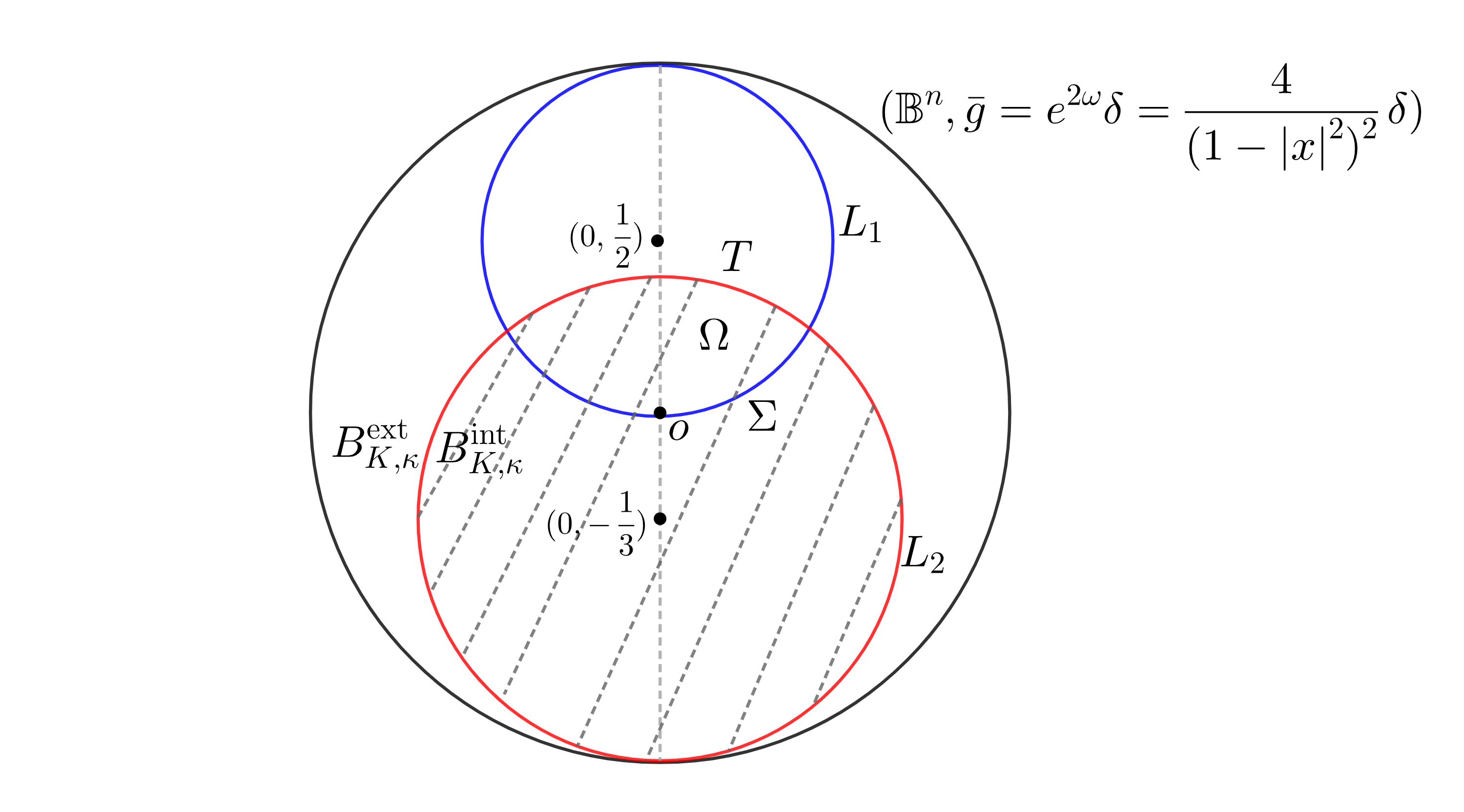
We use the Poincaré ball model (2.2). Let $L_{1}$ and $L_{2}$ be two horospheres as follows

(A.1)		$\displaystyle L_{1}:=\left\{x\in\mathbb{B}^{n}\mid\|x^{\prime}\|^{2}+(x_{n}-\frac{1}{2})^{2}=\frac{1}{4}\right\}$
(A.2)		$\displaystyle L_{2}:=\left\{x\in\mathbb{B}^{n}\mid\|x^{\prime}\|^{2}+(x_{n}+\frac{1}{3})^{2}=\frac{4}{9}\right\}$

$L_{1}$ and $L_{2}$ are mutually orthogonal. See Figure 4.

The domain $\Omega$ is bounded by $\bar{\Sigma}$ and $T$ , that is $\partial\Omega=\bar{\Sigma}\cup T$ , where $\Sigma\subseteq L_{1}$ and $T\subseteq L_{2}$ .

Let

\displaystyle V_{0}:=\frac{1+|x|^{2}}{1-|x|^{2}},\quad V=\frac{2x_{n}}{1-|x|^{2}}.

It is direct to see

(A.3)

\displaystyle|x|^{2}=\frac{V_{0}-1}{V_{0}+1},\quad x_{n}=\frac{V}{V_{0}+1}.

One has the following

Proposition A.1 ([27], Proposition 4.2).

(A.4)

\displaystyle\bar{\nabla}^{2}V_{0}=V_{0}\bar{g},\quad\bar{\nabla}^{2}V=V\bar{g}.

Proposition A.2 ([27] Proposition 4.3).

For any tangential vector field $Z$ on $\mathbb{H}^{n}$ ,

(A.5)		$\displaystyle\bar{\nabla}_{Z}V_{0}=\bar{g}(x,Z);$
(A.6)		$\displaystyle\bar{\nabla}_{Z}V=e^{-\omega}\bar{g}(Z,E_{n})+e^{-2\omega}\bar{g}(x,E_{n})\bar{g}(x,Z).$

Here $e^{2\omega}=\frac{4}{(1-|x|^{2})^{2}}$ .

Let

u:=\frac{1}{n}(V_{0}-V-1)

By Proposition A.1, we have

\bar{\Delta}u-nu=1\quad\text{in}\,\,\Omega.

Combining (A.3) with (A.1), we get

u=0\quad\text{on}\,\,\Sigma\subset L_{1}.

Since $\Sigma\subseteq L_{1}$ and $\bar{g}=e^{2\omega}\delta$ , then the unit outward normal vector of $\Sigma$ is

\nu=2e^{-\omega}(x^{\prime},x_{n}-\frac{1}{2}).

Using (A.5) and (A.6), one checks that on $\Sigma$ ,

(A.7)		$\displaystyle\bar{\nabla}_{\nu}u=\frac{1}{n}(\bar{\nabla}_{\nu}V_{0}-\bar{\nabla}_{\nu}V)=\frac{1}{n}\bar{g}(x,\nu)(1-e^{-2\omega}\bar{g}(x,E_{n}))-\frac{1}{n}e^{-\omega}\bar{g}(\nu,E_{n})$
	$\displaystyle=\frac{2}{n}e^{\omega}(\|x\|^{2}-\frac{1}{2}x_{n})(1-x_{n})-\frac{2}{n}(x_{n}-\frac{1}{2})$
	$\displaystyle=\frac{1}{n}.$

In the last equality above we have used (A.1).

On the other hand, since $T\subseteq L_{2}$ and $\bar{g}=e^{2\omega}\delta$ , then the unit outward normal vector of $T$ is

\bar{N}=\frac{3}{2}e^{-\omega}(x^{\prime},x_{n}+\frac{1}{3}).

Using (A.2), we get

(A.8)

u=\frac{1}{n}(\frac{1+|x|^{2}}{1-|x|^{2}}-\frac{2x_{n}}{1-|x|^{2}}-1)=\frac{5|x|^{2}-1}{n(1-|x|^{2})}\quad\text{on}\,\,T.

Using (A.5), (A.6) and (A.2), one checks that on $T$ ,

(A.9)		$\displaystyle\bar{\nabla}_{\bar{N}}u=\frac{1}{n}(\bar{\nabla}_{\bar{N}}V_{0}-\bar{\nabla}_{\bar{N}}V)=\frac{1}{n}\bar{g}(x,\bar{N})(1-e^{-2\omega}\bar{g}(x,E_{n}))-\frac{1}{n}e^{-\omega}\bar{g}(\bar{N},E_{n})$
	$\displaystyle=\frac{3}{2n}e^{\omega}(\|x\|^{2}+\frac{1}{3}x_{n})(1-x_{n})-\frac{3}{2n}(x_{n}+\frac{1}{3})$
	$\displaystyle=\frac{5\|x\|^{2}-1}{n(1-\|x\|^{2})}.$

Combining (A.8) with (A.9), we get

\bar{\nabla}_{\bar{N}}u=u\quad\hbox{on }T.

In summary, we see $u=\frac{1}{n}(V_{0}-V-1)$ is a solution of the partially overdetermined BVP (1.7), but $\Sigma$ is part of a horosphere. ∎

References

[1] A. D. Alexandrov, Uniqueness theorem for surfaces in the large.V, Vestnik, Leningrad Univ. 13, 19 (1958), 5-8, Amer. Math. Soc. Transl. 21, Ser. 2, 412-416.
[2] M. S. Agranovich, On a mixed Poincare-Steklov type spectral problem in a Lipschitz domain, Russ. J. Math. Phys. 13(3), (2006), 281-290.
[3] N. Aronszajn, A unique continuation theorem for solutions of elliptic partial differential equations, J. Math. Pures. Appl. 36 (1957), pp. 235-249.
[4] J.L.Barbosa and A.G.Colares. Stability of Hypersurfaces with Constant $r$ -Mean Curvature. Annals of Global Analysis and Geometry, 1997, 15(3):277-297.
[5] R. Bañuelos, T. Kulczycki, I. Polterovich, and B. Siudeja. Eigenvalue inequalities for mixed Steklov problems. In Operator theory and its applications, volume 231 of Amer. Math. Soc. Transl. Ser. 2, pages 19-34. Amer. Math. Soc., Providence, RI, 2010.
[6] G.Ciraolo and A.Roncoroni, Serrin’s type overdetermined problems in convex cones, Calc. Var.PDE, 59 (2020), Article: 28.
[7] G. Ciraolo and L. Vezzoni, On Serrin’s overdetermined problem in space forms, manuscripta math. 159 (2019), 445-452.
[8] M.M.Fall, I.A.Minlend, and T.Weth, Serrin’s overdetermined problem on the sphere, Calc.Var.Partial Differential Equation, 57 (2018), no.1, 3.
[9] D.Gilbarg and N.S.Trudinger, Elliptic partial differential equations of second order, Springer, 2015.
[10] P. Grisvard, Elliptic Problems in Nonsmooth Domains, Pitman Advanced Publishing Program, Boston, 1985.
[11] J. Guo and C. Xia, A partially overdetermined problem in a half ball, Calc.Var.Partial Differential Equation. 58 (2019), no.5, 160.
[12] S.E. Koh and S.W. Lee, Addendum to the paper: “Sphere theorem by means of the ratio of mean curvature functions” by Koh, Glasg. Math. J. 43 (2001), no. 2, 275–276.
[13] S.Kumaresan and J.Prajapat, Serrin’s result for hyperbolic space and sphere, Duke Mathematical Journal, 91 (1998) , no.1, 17-28.
[14] J. Li and C. Xia, An integral formula and its applications on sub-static manifolds, J. Differential Geom., 113 (2019), no.3, 493-518.
[15] G. M. Lieberman, Mixed Boundary value problems for elliptic and parabolic differential equations of second order, J. Math. Anal. Appl. 113 (1986), no. 2, 422-440.
[16] R.Lopez, Symmetry of stationary hypersurfaces in hyperbolic space, Geometriae Dedicata, 119 (2006), no.1, 35-47.
[17] S.Montiel and A.Ros, Compact hypersurfaces: the Alexandrov theorem for higher order mean curvatures, In: B. Lawson and K. Tenenblat, Eds., Differential Geometry, Longman, Essex, 1991, pp. 279-296.
[18] R.Molzon, Symmetry and Overdetermined Boundary Value Problems, Forum Mathematicum. 3 (1991) , no.3, 143-156.
[19] F. Pacella and G. Tralli, Overdetermined problems and constant mean curvature surfaces in cones, Rev. Mat. Iberoam. 36 (2020), no. 3, 841-867.
[20] J. Pyo, Rigidity theorems of hypersurfaces with free boundary in a wedge in a space form, Pacific J.Math, 299 (2019), no. 2, 489-510.
[21] G. Qiu and C. Xia, Overdetermined boundary value problems in $\mathbb{S}^{n}$ , J. Math. Study 50 (2017), no. 2, 165-173.
[22] G. Qiu and C. Xia, A generalization of Reilly’s formula and its applications to a new Heintze-Karcher type inequality, Int. Math. Res. Not. IMRN 2015, no. 17, 7608–7619.
[23] R. Reilly, Variational properties of functions of the mean curvature for hypersurfaces in space forms, J. Diffential Geom. 8 (1973), 465šC477.
[24] A. Ros, Compact hypersurfaces with constant higher order mean curvatures, Rev. Mat. Iberoam. 3 (1987) 447–453.
[25] A. Ros and R. Souam, On stability of capillary surfaces in a ball, Pacific J. Math. 178 (1997), No. 2, 345-361.
[26] J. Serrin, A symmetry problem in potential theory, Arch. Ration. Mech. Anal. 43 (1971), 304-318.
[27] G.Wang and C.Xia, Uniqueness of stable capillary hypersurfaces in a ball, Math. Ann. 374(2019), 1845–1882.
[28] G.Wang and C.Xia, Rigidity of free boundary CMC hypersurfaces in a ball, Surveys in Geometric Analysis, 2018, 138-153.
[29] H. Weinberger, Remark on the preceding paper of Serrin,Arch. Ration. Mech. Anal. 43 (1971), 319–320.
[30] H.C.Wente, The symmetry of sessile and pendent drops, Pacific J. Math. 88 (1980), no. 2, 387–397.

A partially overdetermined problem in domains with partial umbilical boundary in space formsThanks: This work is supported by NSFC (Grant No. 11871406).

Abstract.

1. Introduction

Theorem 1.1 ([11]).

Remark 1.1.

Theorem 1.2.

Remark 1.2.

Theorem 1.3.

2. Conformal Killing vector fields in space forms

2.1. Hyperbolic space ℍn\mathbb{H}^{n}

Definition 2.1 ([16]).

Proposition 2.1.

Proof.

Proposition 2.2.

Proof.

2.2. Spherical space 𝕊n\mathbb{S}^{n}

3. Mixed BVP in space forms

Proposition 3.1.

Proof.

Proposition 3.2.

Proof.

Proposition 3.3.

Proof.

Proposition 3.4.

Proof.

Proposition 3.5.

Proof.

4. Partially overdetermined BVP in space forms

Proposition 4.1.

Proof.

Proposition 4.2 ([19], lemma 2.1).

Proposition 4.3.

Proof.

Proposition 4.4.

Proof.

5. Heintze-Karcher-Ros inequality and Alexandrov Theorem

Lemma 5.1 ([23, 4]).

Proposition 5.1.

Proof.

Theorem 5.1.

Proof.

Theorem 5.2.

Proof.

Appendix A An example for BVP with horospheres as boundary

Proposition A.1 ([27], Proposition 4.2).

Proposition A.2 ([27] Proposition 4.3).

References

2.1. Hyperbolic space $\mathbb{H}^{n}$

2.2. Spherical space $\mathbb{S}^{n}$