Abstract
The inverse problem we consider is to reconstruct the location and shape of buried obstacles in the lower half-space of an unbounded two-layered medium in two dimensions from phaseless far-field data. A main difficulty of this problem is that the translation invariance property of the modulus of the far field pattern is unavoidable, which is similar to the homogenous background medium case. Based on the idea of using superpositions of two plane waves with different directions as the incident fields, we first develop a direct imaging method to locate the position of small anomalies and give a theoretical analysis of the algorithm. Then a recursive Newton-type iteration algorithm in frequencies is proposed to reconstruct extended obstacles. Finally, numerical experiments are presented to illustrate the feasibility of our algorithms.
Keywords: Two-layered medium, buried obstacle, phaseless far-field data, direct imaging method, recursive Newton-type iteration algorithm
1 Introduction and main results
In this paper, we consider the inverse scattering by obstacles buried in a two-layered medium separated by a flat plane and filled with different homogeneous materials, which is essential to a broad spectrum of science and technology disciplines like geophysics, underwater acoustics, and obstacle imaging in ocean environments. For simplicity, we will focus our attention on the two-dimensional case.
Let and denote the lower and upper half-spaces, respectively. The interface between the two layers is denoted by . We assume that the scattering obstacle , described by a bounded domain with a connected complement, is fully embedded in the lower half-space .
Consider the incident wave propagating in the direction
| (1.1) |
where is defined as
with being the wave numbers in , respectively. Here, is the wave frequency and are the wave speeds in the half-spaces , respectively. Further, the wave numbers and satisfy with being the refractive index. The scattering problem in the two-layered medium is to find the total field . From the Fresnel formula, is given by
with
where is the reflection direction, is the transmission direction with satisfying that , and the reflection and transmission coefficients and are given by
| (1.2) |
respectively. The scattered wave produced by the interaction of with a sound-soft obstacle in presence of the layered medium satisfies that
| (1.3) |
with , where is the unit normal vector on directed into , denotes the jump across the interface , denotes the circle of radius centered at the origin and the wave number is defined by
The well-posedness of the boundary value problem (1.3) can be obtained by employing a similar argument as in [12] where the case of electromagnetic scattering has been considered. In particular, it can be obtained that the scattered wave has the asymptotic behavior [23]
| (1.4) |
for all directions , where denotes the upper unit half-circle and , defined on , is called the far-field pattern of the scattered wave . In the present paper, given the incident wave , the corresponding scattered wave and far-field pattern are denoted by and , respectively. See Figure 1 for the problem geometry.

In this paper, we are concerned with the inverse scattering problem of recovering the buried obstacle by wave detection made in the upper half-space. This is a difficult problem due to the fact that the problem is both nonlinear and severely ill-posed, which is a typical feature in inverse scattering problems. Various inversion algorithms have been developed to tackle the nonlinearity and ill-posedness, being divided into two types of solution strategies: iteration methods and non-iterative methods. Iteration methods usually make use of nonlinear constrained optimization techniques with suitably choosing regularization terms to tackle the ill-posedness (see, e.g., [21, 22, 20, 46]). Non-iterative methods usually deal with the nonlinearity property without using iteration. Typical examples of non-iterative methods include the linear sampling method [9, 4], the factorization method [30], the method of topological derivatives [1, 3] as well as the MUSIC-type methods [8, 31]. Recently, a new class of sampling methods called direct imaging methods [42, 5, 7, 37] has been widely studied, which is fast and highly robust to noises.
However, in many practical applications, the phase information of the far-field pattern is difficult and sometimes impossible to be measured, and so only the intensity of the far-field pattern (called the phaseless far-field data) is available. Thus, in this paper, we restrict our attention to numerical methods for recovering the scattering obstacle embedded in the two-layered medium from the phaseless far-field data. Inverse scattering with phaseless far-field pattern is more difficult than inverse scattering with full far-field data because of the translation invariance property of the far-field pattern (see Lemma 2.1 below) which makes it impossible to locate the position of the scattering obstacle. Recently, the idea of using a superposition of two different plane waves to be the incident field proposed in [47] can effectively deal with the translation invariance of the far-field pattern. Based on this idea, [47] proposed a Newton method using multi-frequency measured data, whilst [48] developed a direct imaging method to reconstruct the shape and location of the obstacle without knowing the type of boundary conditions in a homogenous background medium. Further, uniqueness can be guaranteed rigorously for recovering obstacles or inhomogeneous media from the intensity of the far-field pattern generated by superpositions of two distinct plane waves (see [43] with certain conditions on the scatterers and [44] without any condition on the scatterers but with a reference ball in the scattering system). In addition, other solution strategies have been proposed to solve inverse scattering problems with phaseless data numerically, such as an iteration method for only shape reconstruction [24, 25], a direct imaging method based on a reference ball technique [27] and a direct imaging method based on the reverse time migration technique [6, 16]. For more results on phaseless inverse scattering problems including the uniqueness issue and other models, see [15, 14, 28, 26, 33, 34, 39, 40, 43, 45, 49].
A large number of contributions exist to deal with the inverse problems in a two-layered background medium. A MUSIC-type algorithm was first studied in [23] to determine the number and locations of small inclusions buried in the lower half-space. An improved MUSIC-type method with multiple frequencies was developed in [41] to image thin inclusions. A direct imaging method was studied in [35] to recover multi-scale buried anomalies, which can locate small inclusions accurately but needs a strong a priori condition for recovering the shape of extended obstacles. An asymptotic factorization method has been considered in [18] in the electromagnetic case. These methods are robust to noises but require some a priori information on the small inclusions. Other work on inverse scattering by extended obstacles can be found in [11, 17, 32, 13], where sampling-type methods and iteration-type methods with phased near-field data have been studied for the layered-medium case. The uniqueness issue was considered in [38] for the case of electromagnetic waves.
To the best of our knowledge, this paper is the first attempt to design an imaging algorithm with the intensity of the far-field pattern to recover the location and shape of an obstacle in a two-layered background medium. Since the translation invariance property is unavoidable, we follow the idea of [43, 47, 48] and consider the incident wave with the incident directions satisfying (1.1). We first extend the direct imaging method in [48] from the homogenous background case to the two-layered medium case to locate multiple small anomalies with the intensity of the far-field pattern measured on the upper half-space. A theoretical analysis of the imaging algorithm is then provided by using the theory of oscillatory integrals. As shown by the results of numerical simulations, the direct imaging algorithm can accurately and effectively determine the number and location of small scatterers. However, the imaging algorithm gives poor shape reconstruction results for extended obstacles, due to the limited aperture measurement data caused by refraction and reflection on the interface . Therefore, in order to obtain better results for the shape reconstruction of an extended obstacle embedded in the lower half-space from the phaseless far-field data, we combine our direct imaging algorithm with the recursive Newton iteration method developed in [47]. Precisely, the initial guess of the Newton iteration method is chosen with the help of the imaging results obtained with the direct imaging algorithm. With such an initial guess, the recursive Newton iteration method can satisfactorily and effectively recover the location and shape of the extended obstacles, as illustrated by the numerical results.
The paper is organized as follows. In Section 2, we introduce the direct imaging method for locating multiple small anomalies and give a theoretical analysis of this method by the theory of oscillatory integrals. In Section 3, a recursive Newton iteration method with multi-frequency phaseless far-field data is developed to recover both the location and the shape of the extended obstacles buried in the lower half-space. Section 4 is devoted to the numerical experiments to illustrate the good performance of the iterative method. Finally, we will give some concluding remarks in Section 5.
2 Locating multiple small anomalies
In this section, we consider the inverse problem for determining the location of multiple small anomalies. For this aim, we introduce the following notations. Let , , be a family of base scatterers such that each is simply connected and has a connected complement. Suppose that represents the multiple disjoint small scatterers, where , and . Further, we also need the following notations for the rest of this paper. For any , belonging to the unit circle , let , with . In particular, for , we define and , where and satisfy the relation
| (2.1) |
And for , we denote and , where is defined by the relation
| (2.2) |
Throughout this paper, the positive constants may be different at different places.
We first stress that the translation invariance property of the phaseless far-field data is inevitable in the two-layered background medium case, as stated by the following lemma.
Lemma 2.1.
Define with . For the incident wave with , the scattered waves and associated with the obstacles and , respectively, satisfy that
| (2.3) |
By Lemma 2.1, we see that it is impossible to determine the location of the obstacle using the modulus of the far-field pattern with only one incident plane wave. Therefore, following the idea of [48], we use the following superposition of two plane waves as the incident field:
with the incident directions . Then, by (1.4) the corresponding scattered wave has the asymptotic behavior
for all directions . By the linear superposition principle it is clear that
| (2.4) |
The inverse problem considered in this paper is to recover the obstacle from the phaseless far-field data for and .
The purpose of this section is to present a direct imaging method with the phaseless far-field data to solve the inverse problem numerically. The imaging function for continuous data is given by
| (2.5) |
where and with and satisfying (2.1), . It follows from (2.4) that for and .
We now study the behavior of for locating multiple small anomalies. We start with the following lemma concerning .
Theorem 2.2.
, where
Here,
are the far-field patterns of the scattering solutions to the scattering problem
| (2.6) |
with the boundary data
| (2.7) | |||
| (2.8) |
respectively.
Proof.
Inserting (2.4) into (2) gives that
Exchanging the order of integration, we have
which is the required equality. Since is the far-field pattern associated with the incident wave , it is easy to obtain that and are the far-field patterns of the scattering solutions to the scattering problem (2.6) with the boundary data given by (2.7) and (2.8), respectively. The proof is complete. ∎
By Theorem 2.2 we know that, in order to investigate the behavior of , it is essential to know the property of the function
| (2.9) |
In fact, it can be shown that decays for large enough. To this end, we need the following result in [6], which is similar to Van der Corput’s lemma for the oscillatory integrals.
Lemma 2.3 (see Lemma 3.9 in [6]).
For any , let be real-valued and satisfy that for all . Assume that is a partition of such that is monotone in each interval , . Then, for the smooth function defined on with integrable derivative and for any , we have
where is a positive constant independent of and .
With the aid of Lemma 2.3, we will prove the following lemma.
Lemma 2.4.
For with large enough, we have
| (2.10) |
where is a constant independent of .
Proof.
Introducing the variable and noting that
we can rewrite as
| (2.11) | |||||
where
Here, is defined as
and . It is easy to obtain that
| (2.12) |
Now the rest of the proof is split into two steps.
Step 1. We first consider the case with . Choose small enough such that and . We distinguish between the following two cases.
Case 1: . From the choice of , we have and thus split (2.11) into three parts:
Set . Then , and is piecewise monotone in . Thus by Lemma 2.3, we have
| (2.13) |
It is easy to show that
| (2.14) |
Combining the estimates (2.12), (2.13) and (2.14) gives
| (2.15) |
Case 2: . We use a similar idea as in the proof of Case 1 and split (2.11) into three parts:
Similarly as in the estimate of in Case 1, it is deduced that
It is easy to see that . Then similarly as in the proof of Case 1, we can obtain the estimate (2.10).
Step 2. Consider the case . Introduce the new variable . Then and
Consequently, the rest proof of this case is similar to the arguments in Step 1. The proof is thus complete. ∎
We now study the behavior of the imaging function . To this end, denote by the fundamental solution of the unperturbed problem (1.3) with , which can be derived by the Fourier transform technique (see, e.g., [36]). Define the single- and double-layer potentials
and the boundary integral operators
It is well known that has the asymptotic formula [23]:
| (2.16) |
where and with and satisfying (2.2).
From Theorem 2.2 it follows that
is the scattering solution to the problem (2.6) with boundary data given by (2.7). From [36] it is known that for and , where
is the fundamental solution of the Helmholtz equation in with being the Hankel function of the first kind of order zero and accounts for the reflection due to the layered medium. Thus it is easy to derive that and are compact perturbations of the corresponding integral operators associated with the homogeneous problem (i.e., with replaced by ). Therefore, by using a similar argument as in the proof of Theorem 3.11 in [10], we can seek the solution in the form of combined double- and single-layer potential with density , that is,
| (2.17) |
where is the unique solution to the boundary integral equation
with given by (2.7). Arguing similarly as in the proof of Theorem 3.11 in [10], we can prove that the operator is bijective and invertible in . Thus we have
| (2.18) |
with two positive constants and independent of .
On the other hand, we have, by Lemma 2.4, that for ,
Let be the distance between and . Then it follows from (2.18) that
| (2.19) |
Since is the far-field pattern of the scattered field , we have
Note that
Then, by (2.19) and the properties of the operators and , it can be seen that decays as moves away from .
Similarly as for the analysis of , it can be seen that
decays as moves away from , where is the symmetric obstacle of with respect to the origin.
From what has been discussed above, it can be seen that the imaging functional decays as moves away from . Further, based on the above analysis, it is reasonable to expect that will take a large value in the neighborhood of . This is confirmed by numerical examples in Section 4 though a rigorous analysis is not available yet. According to the performance of and the fact that , it is enough to determine the location of the obstacle even though the obstacle is completely buried in the lower half-space.
Remark 2.5.
The performance of can also be studied by using the analysis in [35]. In fact, with the aid of Theorem 2.1 in [35] and the smallness assumption on the obstacle , we can easily obtain the following asymptotic formula:
| (2.20) |
for sufficiently large , as , where is given in Theorem 2.2 and , are constants depending on , but independent of . Similar to the proof of Lemma 2.4, it is easy to show that
| (2.21) |
where is a constant independent of and . By (2.20) and (2.21), , , can be seen as a local maximizer in a neighborhood of of defined in Theorem 2.2. Similarly to the above discussion, , , can be seen as a local maximizer in a neighborhood of of defined in Theorem 2.2, where is the symmetric point of with respect to the origin. Therefore, it is expected that multiple small scatterers can be determined by using the imaging functional . This is in accordance with our analysis on .
We are now ready to give the direct imaging algorithm for the inverse problem. Suppose that there are measurement points and sets of two incident directions , where with , with and with . Let . Then with the aid of the trapezoid quadrature rule, the continuous imaging function given in (2) can be approximated by the discrete imaging function defined by
| (2.22) |
where we have employed the facts that and for and . In the numerical experiments, we will consider the noisy phaseless far-field pattern , as the measured data, where is the small perturbation of the phaseless far-field pattern with noise level (see the formula (4.1) below). Accordingly, the discrete imaging function with noisy phaseless far-field data can be computed by (2) with replaced by . Finally, our direct imaging algorithm is based on the discrete imaging function and presented in Algorithm 1.
Remark 2.6.
Since we have the a priori information that the scatterers are embedded in the lower half-space, it is reasonable to choose the sampling region . This, combined with the property of and the fact that , makes it possible to determine the location of the multiple anomalies of the obstacle .
Remark 2.7.
Algorithm 1 can be applied to determine the location of extended obstacle . In fact, by the same analysis discussed above, it is expected that the imaging function decays as moves away from and reaches the local maximums at some points in the neighborhood of . The latter is not yet rigourously proved but will be confirmed by numerical examples in Section 4. With the aid of the a priori information that is embedded in the lower half-space, is able to help us to determine the location of roughly, which will provide our Newton-type iteration method presented in next section with the initial guess.
3 Recovering the location and shape of extended obstacles
As discussed in Remark 2.7, our direct imaging algorithm can determine the location of extended obstacles roughly, providing some a priori information for the iteration-type method. With the aid of the a priori information, we develop a recursive Newton-type iteration algorithm in frequencies to recover the location and shape of extended obstacles embedded in the lower half-space.
Our aim is to solve the nonlinear and ill-posed equation
| (3.1) |
where the far-field operator maps the boundary of the extended scatterer to the corresponding phaseless far-field data induced by the incident wave . For simplicity, we assume that is simply connected in what follows. For the case when the obstacle has several connected components, see the discussion in Remark 3.3.
To proceed further, we need to characterize the Fréchet derivative of the far field operator. Similarly to [47], we choose the Hilbert space of square integrable functions on as the data space, which is suitable for describing the measurement error. Let be a twice continuous differentiable vector field, and define . For a sufficient small depending on , each with is also a -smooth boundary of a domain . Denote the set , then the far field operator is called Fréchet differentiable at if there exists a linear mapping such that for , we have
The following theorem characterizes the Fréchet derivative of the far-field operator .
Theorem 3.1.
Assume that is a -smooth boundary, the incident field is given by with and . Let denote the scattered wave induced by , which solves the problem (1.3) with the boundary data . Then the operator is Fréchet differentiable at with the Fréchet derivative given by , where and is the far-field pattern of solving the problem (1.3) with the boundary data on , where denotes the outward unit normal vector on .
Next, we restrict ourselves to the case when the boundary is a starlike curve, that is, has the form of the following suitable parametrization:
| (3.2) |
with its center at . In numerical computation, similarly to [47], we consider to use multiple sets of incident fields and thus rewrite (3.1) as the following perturbation equation:
| (3.3) |
from a knowledge of the noisy phaseless far-field data , , , which satisfy that
| (3.4) |
with the noise level . Our Newton iteration method consists in using the Levenberg-Marquardt algorithm to solve the linearized equation of (3.3)
| (3.5) |
for , where is the approximation to .
Using the strategy in [47], is taken from a finite-dimensional subspace , , for practical numerical computation, where
with the norm
Then we seek the regularized solution of (3.5) such that is the solution of the minimization problem
| (3.6) |
where the regularization parameter is chosen so that
| (3.7) |
for some parameter and is determined by using the bisection algorithm (see [21]). Thus the approximation can be updated by .
The stopping rule is provided by discrepancy principle (see [21]), that is, the iteration is stopped if , where is a given constant and the relative error is defined by
Remark 3.2.
For the numerical algorithm of this section, we use the layered Green function method in [2] to compute the synthetic data and the numerical solution in each iteration step. To determine the location of the obstacle, we use the measured data , , , , with fixed wave numbers and . For the iteration algorithm proposed in this section, we follow the idea in [47] to make use of the multi-frequency phaseless data , , , with the wave numbers and , . Here, are the same as in Section 2, with , the multiple wave numbers satisfy and is the refractive index. Further, the norm can be approximated by
Based on the above discussions, our numerical algorithm for extend obstacles is presented in Algorithm 2.
for do 4
Remark 3.3.
4 Numerical experiments
4.1 Locating multiple small scatterers
We first present several numerical examples to illustrate the applicability of the direct imaging algorithm (i.e., Algorithm 1) for imaging small scatterers. To generate the synthetic data, the direct scattering problem is solved by the layered Green function method proposed in [2]. As for the far-field data, it is measured with incident and observed directions which are uniformly distributed on and , respectively, that is, and . Further, the noisy phaseless data , , are given as
| (4.1) |
where is noise level and with being standard normal distribution.
Example 1: Locating a small obstacle. We consider the scattering problem by a circle buried in the lower half-space. Our aim is to show that the numerical performance of the imaging function is consistent with our analysis in Section 2, as shown in Figure 4.1. In Figure 4.1, we consider the circle with radius and center at , and the sampling region is chosen to be . Figure 4.1(a) presents the exact position of the small circle. Figure 4.1(b) shows the reconstruction result from the measured data with noise in the case with and . Figure 4.1(c) presents the corresponding imaging result from the measured data with noise in the case with and . It is observed that takes a large value in the neighborhood of and , which is consistent with the analysis in Section 2. With the aid of the a priori information that the obstacle is buried in the lower half-space, we can determine that the position of the small obstacle is .


Example 2: Locating multiple small anomalies in the case . Consider three small circles with radius and centers at , respectively. Here, we choose and . The sampling region is taken to be . Figure 4.2(a) gives the actual position of the three small circles. Figures 4.2(b) and 4.2(c) show the imaging results of the imaging function (2) with using the measured data with noise and with noise, respectively. It is clearly seen from Figure 4.2 that the location and number of the three small scatterers are very well retrieved.


Example 3: Locating multiple small anomalies in the case . Consider three small circles with radius and centers at , respectively. The wave numbers are chosen as and . The sampling region is again taken to be . Figure 4.3 presents the exact position of the three multiple small anomalies and the imaging results given by the imaging function from the measured data with noise and with noise, respectively. Similar to the case in Example 2, the location and number of the three unknown small scatterers are satisfactorily obtained.


4.2 Location and shape reconstruction of extended obstacles
We now carry out numerical implementation for Algorithm 2 presented in Section 3. Shape reconstruction of the obstacles buried in the lower half-space will be considered in two cases: and . The corresponding far-field pattern is computed by the layered Green function method given in [2] with the number of collocation points doubled in order to avoid inverse crime. Noisy phaseless data with noise level are simulated by using (4.1), which satisfy the condition (3.4) approximately. In all numerical examples, we choose the parameters , , , , , and in Algorithm 2. In the case , we choose the refractive index and use multi-frequency data with . And the noisy phaseless far-field data 2 are generated by the incident waves with three different sets of incident directions (i.e., ) with , , , , , . In the case , the refractive index is chosen as , and we use multi-frequency phaseless data 2 with . And the noisy phaseless far-field data 2 are measured by using four different sets of incident directions (i.e. ) with , , , , , , , . We recall that, according to the settings in Section 3, if the wave number in is given by () then the wave number in is given by . The parametrization of the test curves for the boundary is given in Table 4.1.
| Type | Parametrization |
|---|---|
| Ellipse | |
| Apple shaped | |
| Rounded triangle | |
| Rounded square |
Example 4: Reconstruction of an obstacle in the case Consider the inverse problem for reconstructing the apple-shaped obstacle in the case . Figure 4.4(a) presents the imaging result in the sampling region by the direct imaging algorithm with , whose local maximum is at . Figures 4.4(b) and 4.4(c) present the initial curve and the reconstruction result at , respectively, where the solid line represents the exact curve. It can be seen from Figure 4.4(c) that the location and shape of the obstacle are satisfactorily reconstructed.


Example 5: Reconstruction of an obstacle in the case . Consider the inverse problem in the case , where the obstacle is the same as in Example 4. Figure 4.5(a) presents the imaging result by the direct imaging method with , whose local maximum is at . Figures 4.5(b) and 4.5(c) present the initial curve and the reconstruction result at , respectively, where the solid line represents the exact curve. It can be seen from Figure 4.5(c) that only the upper part of the obstacle can be satisfactorily reconstructed.


Example 6: Reconstruction of multiple obstacles in the case . We now consider the inverse problem for reconstructing multiple obstacles consisting of an ellipse-shape, a rounded triangle-shape and a rounded square-shape in the case . Figure 4.6(a) presents the imaging result by Algorithm 1 with , whose local maximums are at , respectively. Figures 4.6(b) and 4.6(c) present the initial curve and the reconstruction result at , respectively, where the solid line represents the exact curve. It is seen from Figure 4.6(c) that the location and shape of the rounded triangle-shaped and ellipse-shaped obstacles are satisfactorily reconstructed. However, the lower part of the rounded square-shaped obstacle is not very accurately reconstructed compared with its upper part.

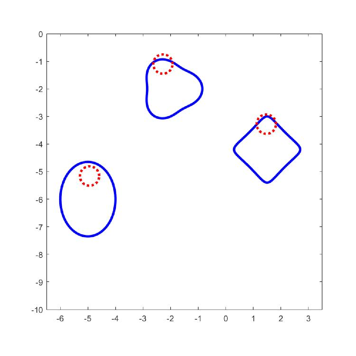

Example 7: Reconstruction of multiple obstacles in the case . Consider the inverse problem for reconstructing multiple obstacles in the case , where the obstacles are the same as in Example 6. Figure 4.7(a) presents the imaging result by the direct imaging method with , whose local maximums are at , respectively. Figures 4.7(b) and 4.7(c) present the initial curve and the reconstruction result at , where the solid line represents the exact curve. From Figure 4.7(c) it is concluded that the upper part of the shape for all obstacles can be satisfactorily reconstructed, which is consistent with the results in Example 5. Further, both the location and shape of the rounded triangle-shaped obstacle are reconstructed very well. However, the lower parts of the ellipse-shaped and rounded square-shaped obstacles are not very accurately reconstructed.


5 Conclusions and future work
In this paper, we have proposed two algorithms to image buried obstacles in the lower half-space of an unbounded two-layered medium with only phaseless far-field data. Following the idea of [47], we make use of superpositions of two plane waves as the incident fields and extend the direct imaging algorithm in [48] and the recursive Newton-type iteration method in [47] to the two-layered medium problem. The direct imaging method can determine the location of the buried obstacles, providing some a priori information for the recursive iteration method. Combining this a priori information with the recursive Newton-type iteration method, the location and shape of the extended obstacles buried in the lower half-space can be recovered.
Through various numerical experiments, it has been shown that both two algorithms proposed in this paper are effective not only for the case but also for the case . However, it is observed that the reconstruction results for the case are better than those for the case . In particular, for the case , the lower part of the obstacle is not very accurately reconstructed compared with its upper part. This may be due to the fact that the phaseless far-field data are only measured on the upper unit half-circle. Therefore, certain improvements still need to be further investigated.
Acknowledgments
The work of L. Li and J. Yang is partially supported by the NNSF of China grants 11961141007 and 61520106004, and Microsoft Research of Asia. The work of H. Zhang is supported by the NNSF of China grant 11871466.
References
- [1] H. Ammari, J. Garnier, V. Jugnon and H. Kang, Stability and resolution analysis for a topological derivative based imaging functional, SIAM J. Control Optim. 50 (2012), 48-76.
- [2] C.A.P. Arancibia, Windowed Integral Equation Methods for Problems of Scattering by Defects and Obstacles in Layered Media, PhD Thesis, California Institute of Technology, USA, 2017.
- [3] C. Bellis, M. Bonnet and F. Cakoni, Acoustic inverse scattering using topological derivative of far-field measurements-based -cost functionals, Inverse Problems 29 (2013) 075012.
- [4] F. Cakoni and D. Colton, A Qualitative Approach to Inverse Scattering Problem, Springer, Berlin, 2014.
- [5] J. Chen, Z. Chen and G. Huang, Reverse time migration for extended obstacles: acoustic waves, Inverse Problems 29 (2013) 085005.
- [6] J. Chen, Z. Chen and G. Huang, Phaseless imaging by reverse time migration: Acoustic waves, Numer. Math. Theor. Meth. Appl. 10 (2017), 1-21.
- [7] Z. Chen and G. Huang, Reverse time migration for reconstructing extended obstacles in the half space, Inverse Problems 31 (2015) 055007.
- [8] M. Cheney, The linear sampling method and the MUSIC algorithm, Inverse Problems 17 (2001), 591-595.
- [9] D. Colton and A. Kirsch, A simple method for solving inverse scattering problems in the resonance region, Inverse Probl. 12 (1996), 383-393.
- [10] D. Colton and R. Kress, Inverse Acoustic and Electromagnetic Scattering Theory (3rd edn), Springer, Berlin, 2013.
- [11] J. Coyle, Locating the support of objects contained in a two-layered background medium in two dimensions, Inverse Problems 16 (2000), 275-292.
- [12] P.-M. Cutzach and C. Hazard, Existence, uniqueness and analyticity properties for electromagnetic scattering in a two-layered medium, Mathematical Methods in the Applied Sciences 21 (1998), 433-461.
- [13] F. Delbary, K. Erhard, R. Kress, R. Potthast and J. Schulz, Inverse electromagnetic scattering in a two-layered medium with an application to mine detection, Inverse Problems 24 (2007) 015002.
- [14] H. Dong, J. Lai and P. Li, Inverse obstacle scattering for elastic waves with phased or phaseless far-field data, SIAM J. Imaging Sci. 12 (2019), 809-838.
- [15] H. Dong, D. Zhang and Y. Guo, A reference ball based iterative algorithm for imaging acoustic obstacle from phaseless far-field data, Inverse Probl. Imaging 13 (2019), 177-195.
- [16] S. Fang, Z. Chen and G. Huang, A direct imaging method for the half-space inverse scattering problem with phaseless data, Inverse Probl. Imaging 11 (2017), 901-16.
- [17] B. Gebauer, M. Hanke, A. Kirsch, W. Muniz and C. Schneider, A sampling method for detecting buried objects using electromagnetic scattering, Inverse Problems 21 (2005), 2035-2050.
- [18] R. Griesmaier, An asymptotic factorization method for inverse electromagnetic scattering in layered media, SIAM J. Appl. Math. 68 (2008), 1378-1403.
- [19] F. Hettlich, Frechet derivatives in inverse obstacle scattering, Inverse Problems 11 (1995), 371-382.
- [20] T. Hohage, Convergence rates of a regularized newton method in sound-hard inverse scattering, SIAM J. Numer. Anal. 36 (1998), 125-142.
- [21] T. Hohage, Iterative Methods in Inverse Obstacle Scattering: Regularization Theory of Linear and Nonlinear Exponentially Ill-Posed Problems, PhD Thesis, University of Lintz, Austria, 1999.
- [22] T. Hohage and C. Schormann, A Newton-type method for a transmission problem in inverse scattering, Inverse Problems 14 (1998), 1207-1227.
- [23] E. Iakovleva, H. Ammari and D. Lesselier, A MUSIC algorithm for locating small inclusions buried in a half-space from the scattering amplitude at a fixed frequency, SIAM Multiscale Model. Simul. 3 (2005), 597-628.
- [24] O. Ivanyshyn, Shape reconstruction of acoustic obstacles from the modulus of the far field pattern, Inverse Probl. Imaging 1 (2007), 609-622.
- [25] O. Ivanyshyn and R. Kress, Identification of sound-soft 3D obstacles from phaseless data, Inverse Probl. Imaging 4 (2010), 131-149.
- [26] X. Ji, X. Liu and B. Zhang, Phaseless inverse source scattering problem: Phase retrieval, uniqueness and direct sampling methods,J. Comput. Phys. X 1 (2019) 100003.
- [27] X. Ji, X. Liu and B. Zhang, Target reconstruction with a reference point scatterer using phaseless far field patterns, SIAM J. Imaging Sci. 12 (2019), 372-391.
- [28] X. Ji, X. Liu and B. Zhang, Inverse acoustic scattering with phaseless far field data: Uniqueness, phase retrieval, and direct sampling methods, SIAM J. Imaging Sci. 12 (2019), 1163-1189.
- [29] A. Kirsch, The domain derivative and two applications in inversescattering theory, Inverse Pmblem 9 (1993), 81-96.
- [30] A. Kirsch, Characterization of the shape of a scattering obstacle using the spectral data of the far field operator, Inverse Problems 14 (1998), 1489-1512.
- [31] A. Kirsch, The MUSIC-algorithm and the factorization method in inverse scattering theory for inhomogeneous media, Inverse Problems 18 (2002), 1025-1040.
- [32] A. Kirsch, An integral equation for maxwell equations in a layered medium with an application to the factorization method, J. Integral Equations Appl. 19 (2007), 333-57.
- [33] M.V. Klibanov, Phaseless inverse scattering problems in three dimensions, SIAM J. Appl. Math. 74 (2014), 392-410.
- [34] M.V. Klibanov, A phaseless inverse scattering problem for the 3-D Helmholtz equation, Inverse Probl. Imaging 11 (2017), 263-276.
- [35] J. Li, P. Li, H. Liu and X. Liu, Recovering multiscale buried anomalies in a two-layered medium, Inverse Problems 31(2015) 105006.
- [36] P. Li, Coupling of finite element and boundary integral method for electromagnetic scattering in a two-layered medium, J. Comput. Phys. 229 (2010), 481-497.
- [37] X. Liu, A novel sampling method for multiple multiscale targets from scattering amplitudes at a fixed frequency, Inverse Problems 33 (2017) 085011.
- [38] X. Liu and B. Zhang, A uniqueness result for the inverse electromagnetic scattering problem in a two-layered medium, Inverse Problems 26 (2010) 105007.
- [39] R.G. Novikov, Formulas for phase recovering from phaseless scattering data at fixed frequency, Bull. Sci. Math. 139 (2015), 923-936.
- [40] R.G. Novikov, Explicit formulas and global uniqueness for phaseless inverse scattering in multidimensions, J. Geom. Anal. 26 (2016), 346-359.
- [41] W.-K. Park, On the imaging of thin dielectric inclusions buried within a half-space, Inverse Problems 26 (2010) 074008.
- [42] R. Potthast, A study on orthogonality sampling, Inverse Problems 26 (2010) 074015.
- [43] X. Xu, B. Zhang and H. Zhang, Uniqueness in inverse scattering problems with phaseless far-field data at a fixed frequency, SIAM J. Appl. Math. 78 (2018), 1737-1753.
- [44] X. Xu, B. Zhang and H. Zhang, Uniqueness in inverse scattering problems with phaseless far-field data at a fixed frequency. II, SIAM J. Appl. Math. 78 (2018), 3024-3039.
- [45] X. Xu, B. Zhang and H. Zhang, Uniqueness and direct imaging method for inverse scattering by locally rough surfaces with phaseless near-field data, SIAM J. Imaging Sci. 12 (2019), 119-152.
- [46] B. Zhang and H. Zhang, A Newton method for a simultaneous reconstruction of an interface and a buried obstacle from far-field data, Inverse Problems 29 (2013) 045009.
- [47] B. Zhang and H. Zhang, Recovering scattering obstacles by multi-frequency phaseless far-field data, J. Comput. Phys. 345 (2017), 58-73.
- [48] B. Zhang and H. Zhang, Fast imaging of scattering obstacles from phaseless far-field measurements at a fixed frequency, Inverse Problems 34 (2018) 104005.
- [49] D. Zhang and Y. Guo, Uniqueness results on phaseless inverse acoustic scattering with a reference ball, Inverse Problems 34 (2018) 085002.