Causal query in observational data with hidden variables

We use upper case letters to represent variables and bold-faced upper case letters to denote sets of variables. Let $\mathcal{G}=(\mathbf{V},\mathbf{E})$ be a graph, where $\mathbf{V}=\{V_{1},\dots,V_{p}\}$ is the set of nodes and $\mathbf{E}$ a set of edges. Two nodes are adjacent if there is an edge between them. The set of all the nodes adjacent to node $V$ is denoted as $Adj(V)$. A path $\pi$ from $V_{s}$ to $V_{e}$ is a sequence of distinct nodes $<V_{s},\dots,V_{e}>$ such that every pair of successive nodes are adjacent in $\mathcal{G}$. A sub-path of $\pi$ from $V_{i}$ to $V_{j}$ is denoted by $\pi(V_{i},V_{j})$. In $\mathcal{G}$, if there exists $V_{i}\rightarrow V_{j}$, $V_{i}$ is a parent of $V_{j}$ and we use $Pa(V_{j})$ to denote the set of all parents of $V_{j}$. If there exists $V_{i}\leftrightarrow V_{j}$, $V_{i}$ is a spouse of $V_{j}$ and we use $Sp(V_{j})$ to denote the set of all spouses of $V_{j}$. A path from $V_{s}$ to $V_{e}$ is a directed path if for any pair of adjacent nodes $V_{i}$ and $V_{j}$ in the path where $i\leq j$, $V_{i}$ is a parent of $V_{j}$. $V_{s}$ is an ancestor of $V_{e}$ if there is a directed path from $V_{s}$ to $V_{e}$. The ancestor set of $V_{e}$ is denoted as $An(V_{e})$.

A DAG is a directed graph without directed cycles (See an example of directed cycle in Figure 1 (a)). When a DAG satisfies the following Markov condition and faithfulness assumption, we can read dependency/independency in a distribution from the DAG.

Based on the Markov condition, according to $\mathcal{G}$ $\textsl{P}(\mathbf{V})$ can be factorized into: $\textsl{P}(\mathbf{V})=\prod_{i}p(V_{i}|Pa(V_{i}))$.

A causal DAG is a DAG in which a node’s parents are interpreted as its direct causes. To learn a causal DAG from observational data, we also need to assume causal sufficiency.

When causal sufficiency is violated, ancestral graphs are used to represent data generating processes. An ancestral graph $\mathcal{M}$ is a mixed graph that does not contain directed cycles or almost directed cycles. A graph is called a mixed graph if it includes directed and bi-directed edges. When there exists a bi-directed edge $V_{i}\leftrightarrow V_{j}$ in $\mathcal{M}$, there is not directed path $V_{i}\rightarrow V_{j}$ or $V_{i}\leftarrow V_{j}$. An almost directed cycle occurs when $V_{i}\leftrightarrow V_{j}$ is in $\mathcal{M}$ and $V_{j}\in An(V_{i})$, Figure 1 (b) is such an example. Let “$\ast$” denote any allowed edge marks. For a path $\pi$, a non-ending node $V_{i}$ is a collider on $\pi$ if $\pi$ contains $V_{i-1}\put(0.2,-2.5){*}\rightarrow V_{i}\leftarrow\put(-3.6,-2.5){*}V_{i+1}$. A path $\pi$ is a collider path if each node excluding the ending nodes on $\pi$ is a collider.

If $V_{i}$ and $V_{j}$ are m-separated by $\mathbf{Z}$, $V_{i}\mathbin{\mathchoice{\hbox to0.0pt{\hbox{$\displaystyle\perp$}\hss}\kern 3.46875pt{}\kern 3.46875pt\hbox{$\displaystyle\perp$}}{\hbox to0.0pt{\hbox{$\textstyle\perp$}\hss}\kern 3.46875pt{}\kern 3.46875pt\hbox{$\textstyle\perp$}}{\hbox to0.0pt{\hbox{$\scriptstyle\perp$}\hss}\kern 2.48856pt{}\kern 2.48856pt\hbox{$\scriptstyle\perp$}}{\hbox to0.0pt{\hbox{$\scriptscriptstyle\perp$}\hss}\kern 1.78203pt{}\kern 1.78203pt\hbox{$\scriptscriptstyle\perp$}}}V_{j}|\mathbf{Z}$, the information flow from $V_{i}$ and $V_{j}$ is “blocked” by $\mathbf{Z}$. In this paper, we call $\mathbf{Z}$ a block set of the ordered pair ($V_{i},V_{j}$).

We present an example of causal MAG in Figure 2 (b). Figure 2 (a) is its corresponding causal DAG with the hidden variables $U_{1}$ and $U_{2}$ shown. In a MAG $\mathcal{M}$, if a path between $V_{s}$ and $V_{e}$ is a directed path, it is called a causal path from $V_{s}$ to $V_{e}$. A non-directed path between $V_{s}$ and $V_{e}$ is a non-causal path. In Figure 2(b), path $W\rightarrow Y$ is a causal path, and other paths between $W$ and $Y$ are non-causal paths.

Figure 3 shows two different graphical configurations where the edge $V_{i}\rightarrow V_{j}$ is visible. In a given MAG $\mathcal{M}$, a visible edge $V_{i}\rightarrow V_{j}$ implies that there are no hidden variables between $V_{i}$ and $V_{j}$. Otherwise, the edge $V_{i}\rightarrow V_{j}$ may include hidden variables.

Let $W$ be a binary treatment variable, $Y$ the outcome variable. The causal effect of $W$ on $Y$, $CE(W,Y)$ is the change of $Y$ due to a change of $W$. When we use the do operator [25] to represent a manipulation of a variable (e.g. set $W$ to 1) and denote $W=1$ and $W=0$ as $w,w^{\prime}$ respectively, $CE(W,Y)$ is defined as:

When estimating the causal effect of W on Y, the effect of other variables needs to be eliminated or adjusted to obtain an unbiased estimation of the causal effect. In graphical causal modelling, the back-door criterion is the main principle for identifying a set of adjustment variables, denoted as $\mathbf{Z}$ in this paper.

Given an adjustment set $\mathbf{Z}$, the causal effect $CE(W,Y)$ can be estimated unbiasedly as follows:

When the assumption of causal sufficiency does not hold, the generalised back-door criterion in a MAG can be used to search for an appropriate adjustment set $\mathbf{Z}$ for estimating $CE(W,Y)$ [22].

If a set $\mathbf{Z}$ in $\mathcal{M}$ satisfies the generalised back-door criterion, relative to $(W,Y)$, then the unbiased estimation of $CE(W,Y)$ can be achieved by Eq.(2).

In some MAGs, the adjustment sets could not be found due to the causal ambiguities, and this can be judged based on the amenability of a MAG [35] as defined below.

If the MAG $\mathcal{M}$ is not adjustment amenable w.r.t. $(W,Y)$, then no adjustment set $\mathbf{Z}$ in $\mathbf{V}\setminus\{W,Y\}$ can be found [35].

Let $\mathbf{D}$ be a dataset containing a binary treatment variable $W$, an outcome variable $Y$ which is binary or numerical, and $\mathbf{X}$, a set of all other variables of any type. We assume that the dataset is generated from an underlying causal MAG M which is adjustment amenable to the ordered pair $(W,Y)$. We also assume that all the variables in $\mathbf{X}$ are measured before applying the treatment and observing $Y$, indicating that variables in $\mathbf{X}$ are all non-descendants of $W$ or $Y$ in $\mathcal{M}$. The pretreatment variable assumption is realistic as it reflects what normally happens in practice, that is, all the other variables are often measured before the treatment is applied and the outcome is observed. This assumption is commonly used in [9, 12, 14, 36].

In the proposed Theorem 1 below, $\mathcal{M}_{\underline{W}}$ denotes the manipulated $\mathcal{M}$ from which $W\rightarrow Y$ has been removed, and $\mathcal{M}_{\underline{W}}$ is still a MAG by the closure property of a MAG [27].

Based on the above Theorem developed, we can firstly employ a local causal structure discovery algorithm to obtain $Adj(W\cup Y)$ from data, then our answer to a causal query is an Adjustment Set-Causal Effect Table, or ASCET, where each row contains a candidate adjustment set (a subset of $Adj(W\cup Y)$) and the causal effect estimated corresponding to the candidate adjustment set.

Example. Suppose $Adj(W\cup Y)=\{X_{1},X_{2},X_{3}\}$, Table 3.3 shows an example ASCET where 1 denotes a variable is in a candidate adjustment set and 0 otherwise.

We reduce the size of ASCET by removing variables that do not significantly affect causal effect estimation. To test if a variable significantly affects causal effect estimation, we compare the cause effect estimated by including the variable with the cause effect estimated by excluding the variable in all cases. If the average difference is smaller than a threshold, the variable is insignificant. More precisely, we have the following definition.

The sensitivity of variable $X$ reflects its impact on the estimated causal effect of $W$ on $Y$. When $X$ has a low sensitivity, no significant error will be introduced if we exclude it from $Adj(W\cup Y)$. So, $X$ is removed from $Adj(W\cup Y)$, and the size of ASCET is reduced.

Example. We use the example in Table 3.3 to illustrate how we reduce the size of ASCET. We use $X_{1}$ as an example, $\rho=4$ as the size of the power set of $\{X_{2},X_{3}\}$ is 4, then $Sen(X_{1})=\frac{1}{4}(|CE_{\{X_{1}\}}-CE_{\phi}|+|CE_{\{X_{1},X_{2}\}}-CE_{\{X_{2}\}}|+|CE_{\{X_{1},X_{3}\}}-CE_{\{X_{3}\}}|+|CE_{\{X_{1},X_{2},X_{3}\}}-CE_{\{X_{2},X_{3}\}}|)=\frac{1}{4}(0.1+0+0.4+0.4)=0.25$. In the same way, $Sen(X_{2})=0.025$ and $Sen(X_{3})=0.175$. Hence, $X_{2}$ has a low sensitivity such that we can exclude it from $Adj(W\cup Y)$ and the corresponding rows in ASCET can be removed. The final result is presented as Table 3.3.

Algorithm 1 presents our proposed algorithm for Data-drIven Causal Effect estimation without causal sufficiency (DICE). DICE contains two parts. Part 1 (lines 1 to 13) is for finding $Adj(W\cup Y)$. Firstly, a local causal structure learning algorithm (such as PC-Select [4] or HITON-PC [1]) is used to find the parents of $W$ and $Y$. In this work, we use PC-Select, given its high accuracy, PC-Select is a local version of PC [32], an algorithm for learning a global causal structure. Then we check whether $Adj(W)=Adj(W)\setminus\{Y\}$ is empty to determine if the causal effect of $W$ on $Y$ is identifiable or not from data. If $Adj(W)$ is empty, no adjustment set can be found, and DICE returns an empty ASCET and terminates.

Part 2 of Algorithm 1 (lines 7 to 16) firstly estimates each possible causal effect when adjusting each subset of $Adj(W\cup Y)$. We use Propensity Score Matching (PSM) [28] to estimate causal effects where propensity score is calculated by glm and matching is performed by Match in the $\mathbb{R}$ packages stats and Matching [30], respectively. The adjustment sets and the corresponding causal effects estimated are added to the ASCET. Next, DICE calculates the sensitivity of each variable in $Adj(W\cup Y)$, and if a variable’s sensitivity is below the given threshold, DICE removes all the adjustment sets containing the variable and the corresponding causal effects from the ASCET.

Time-complexity analysis. PC-Select and PSM contribute the most to the time complexity of DICE. In the worst case, the complexity of PC-Select is $\mathbf{O}(p2^{p-1}n)$ [4], where $p$ is the number of variables and $n$ the number of samples. In our problem, the worst case is when all variables of $\mathbf{X}$ are causes of $W$ and/or $Y$, which, however rarely occurs. In most cases, PC-Select can handle thousands of variables [4]. The time complexity of PSM is $\mathbf{O}(p^{2})$. Our experiment in Section 4 shows that DICE scales with both $p$ and $n$ well.

Before evaluating DICE, we assess the quality of local structure learning algorithm, i.e. PC-Select used in our paper versus global structure learning algorithms. The synthetic datasets are generated according to the underlying causal DAG in Fig 2 (a) with 8 pretreatment variables, 2 hidden variables, $W$ and $Y$ by following the procedure in [11]. The underlying causal MAG is presented in Fig 2 (b), i.e. $U_{1}$ and $U_{2}$ are removed from these generated datasets.

We generate two groups of datasets to evaluate the impact of sample size and the number of variables on the quality of the local structure learning algorithm, respectively. The first group of datasets include 10 datasets , each containing 5K samples for 10 variables generated from Fig 2(b), plus 0, 10, 20, $\dots$, 90 random variables, respectively. The second group of datasets include 20 datasets with 10 fixed variables of the MAG, but with varying sample sizes of 5K, 10K, $\dots$, 95K and 100K. These datasets with hidden variables are used to evaluate the quality of the local structure learning algorithm.

We use two global structure learning algorithms, Fast causal inference (FCI) [32] and Really FCI (RFCI) [8] to learn from each of the generated datasets a PAG (Partial Ancestral Graph) which represents a Markov equivalence class of MAGs encoding the same dependence/independence relations in the data. Then we extract $Adj(W)$ and $Adj(Y)$ from the learned PAG. For PC-Select, we apply it twice to a dataset, one having $W$ as the target and the other having $Y$ as the target to learn $Adj(W)$ and $Adj(Y)$. The implementations of FCI, RFCI and PC-Select are from the $\mathbb{R}$ package pcalg [17], with the default parameter settings and a significance level ($\alpha$) of 0.05.

Results. We perform the experiments 10 times on each of the 30 datasets. We draw the mean results (precision, recall and F-score) of the three algorithms in Figure 4. The local structure learning algorithm PC-Selects achieves similar performance as the global structure learning algorithm in $Adj(W)$ and $Adj(Y)$, indicating that adjustment set discovery in data by local search is reliable.

We evaluate the effectiveness of DICE on three real-world datasets: Jobs training (Jobs for short) [18], IHDP [12] and Twins [2]. A brief description of the datasets is shown in Table 3.

Jobs consists of the original LaLonde dataset (297 treated samples and 425 control samples) [18] and the Panel Study of Income Dynamics (PSID) observational group (2490 control samples) [14]. Each sample has 9 variables, including 7 pretreatment variables (which are age in years, schooling in years, indicators for black and Hispanic, marriage status, school degree, previous earnings in 1974 and 1975, and whether the 1974 earnings variable is missing), employment status with/without job training as treatment variable, and 1978 earning as the outcome variable. Because the dataset contains records of people taking part in the training only, as in [18], we estimate Average Treatment Effect on Treated (ATT) for DICE and all comparisons, against the ground truth ATT which is $886 [14].

IHDP is related to the Infant Health and Development Program (IHDP) on low-birth-weight premature infants [12]. IHDP has 24 pretreatment variables and we follow the method in [12] to generate the simulated outcome with the ground-truth of 4.38 for the causal effect (CE) by the $\mathbb{R}$ package npci¹¹ 1 https://github.com/vdorie/npci.

The Twins dataset consists of samples from twin births in the USA between 1989 and 1991 with the birth weight less than 2000g [2]. We eliminate records with missing values and have 4821 twin pairs left. The treatment variable is birth weight: W=1 for a baby who is heavier in a twin; W=0 otherwise. The mortality after one year is the true outcome for each twin, and the ground-truth causal effect is -0.025. To simulate an observational study, according to [21], we use the following Bernoulli distribution to randomly select one of the two twins as the observation and hide the other: $W_{i}|x_{i}\sim Bern(sigmoid(\beta^{T}\mathbf{x}+\varepsilon))$, where $x_{i}$ denotes the pre-treatment variables of the sample $i$, $\mathbf{x}$ denotes the samples set, and $\beta^{T}\sim\mathcal{U}((-0.1,0.1)^{40\times 1})$ and $\varepsilon\sim\mathcal{N}(0,0.1)$.

There are two major objectives for the experiments.

Firstly, we will show that the true adjustment set can be found as shown in Theorem 1, and therefore the smallest bias of DICE will be very small. We compare DICE with a data-driven causal effect estimation method, LV-IDA [24]²² 2 https://github.com/dmalinsk/lv-ida which uses FCI to learn a PAG and searches for an adjustment set in each MAG enumerated from the PAG. LV-IDA returns a set of causal effects, one for the adjustment set discovered from each MAG. In the experiment, we report the best estimates for both methods to show the quality of adjustment sets found.

Secondly, we will show that a causal effect estimated by DICE is comparative with the best estimates by methods using domain knowledge. Some statistical and machine learning methods are available for causal effect estimation, with the assumptions of known covariate set and unfoundedness. The typical methods include PSM, propensity score matching with logistic regression [28]; CBPS, covariate balancing propensity score [14]; CFRNET, a deep learning framework for counterfactual regression with a theoretical error bound (named as CFR) [31]; LASSO, Linear regression with the regularization $\ell_{1}$-norm to predict the factual outcome [33]; BART, Bayesian additive regression tree [7], a non-linear model which has been applied for counterfactual inference [12]; TMLE, targeted maximum likelihood estimation, a doubly robust method [34]; CausalForest, Random forest regression to estimate causal effect [37] (CF for short). In the experiments, we compare DICE with all the above mentioned methods.

The three datasets will favour the above methods since the unconfoundedness assumption is satisfied. Since the datasets were obtained from well designed observational studies and the covariates were chosen by domain experts.

DICE returns ASCET, the set of adjustment set and causal effect pairs. When reporting causal effects estimated by DICE, we use the most probable value in the ASCET after removing insignificant variables with the sensitivity threshold of $\tau=0.1$. We group the causal effect in the ASCET by using the bin size of $(\max(Y)/100)$. The average causal effect in the most frequent bin is used as an estimated causal effect.

The parameter setting of DICE is that the Match function of estimate is set to “ATT” for Jobs and “ATE” for IHDP and Twins as in the prior work in [12, 31]. Other parameters are set as the default. For CF, the parameter num.trees is set from 10 to 300 with the increment of 10, and the best result is reported. For PSM and CBPS, all variables are included in the adjustment variable set.

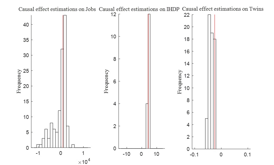
The experimental results are shown in Tables 4, 5, 6, and Figure 5. From the results, we have the following conclusions.

Firstly, DICE finds the correct adjustment set through local search. Comparing with the other methods, the lowest biases of DICE are consistently the smallest in the three datasets, and are significantly smaller than the lowest biases of LV-IDA, which searchers adjustment sets by global search.

Secondly, causal effects estimated by DICE are comparative with those by other methods which make use of domain knowledge. For the IHDP dataset, DICE achieves the smallest bias. For the Jobs dataset, DICE is ranked the 3rd based on smallest biases. For the Twin dataset, the largest absolute bias is only 0.015, and hence we consider that the estimates by all methods are similar and good.

To show that those comparison methods do not work in a dataset when the unconfoundedness assumption is not satisfied, we have generated datasets with $M$-bias [26]. The performance of some methods deteriorates greatly. Implementations of other methods do not work with datasets with more than 200K records. We do not show the results in this paper due to the space limitation.

As PC-Select is a major contributor to the complexity of DICE, in this section, we firstly evaluate the efficiency of PC-Select, and then the overall efficiency of DICE. The computations were performed on a PC with 2.6 GHz Intel Core i7 and 16GB of memory.
Efficiency evaluation of the structure learning algorithms.. We record the running time of the structure learning algorithms on the synthetic datasets introduced in Section 4.1 and draw the mean running time in Figure 6. PC-Select is faster than FCI and RFCI, and comparing to FCI and RFCI, PC-Select scales with the number of variables and samples very well.

Experiments on ten standard benchmark BNs. To evaluate the efficiency of DICE, we use the datasets generated from the ten benchmark BNs from the BN repository³³ 3 http://www.bnlearn.com/bnrepository/: SACHS, CHILD, INSURANCE, WATER, ALARM, BARLEY, HAILFINDER, HEPAR II, WIN95 and ANDES. With each BN, we choose a variable without child nodes as the outcome variable and then select one of its parents without child nodes (except the outcome) as the treatment variable. We generate ten synthetic datasets from the ten BNs with 5000 samples each using the $\mathbb{R}$ package bnlearn [29]. Then we hide 5% variables (only one variable is hidden for the small BNs SACHS and CHILD) which lie on a non-causal path between the treatment and outcome variables. The same parameter settings are used for DICE and LV-IDA as in Subsection 4.2.

Results. As shown in Figure 7, DICE is faster than LV-IDA across all the 10 datasets. Especially, LV-IDA did not return results for the 5 datasets generated using the larger BNs within two hours, while DICE completed in seconds (at most 50+ seconds) for all datasets.

References

- [1] Constantin F Aliferis, Alexander Statnikov, Ioannis Tsamardinos, Subramani Mani, and Xenofon D Koutsoukos, ‘Local causal and markov blanket induction for causal discovery and feature selection for classification part i: Algorithms and empirical evaluation’, Journal of Machine Learning Research, 11(Jan), 171–234, (2010).
- [2] Douglas Almond, Kenneth Y Chay, and David S Lee, ‘The costs of low birth weight’, The Quarterly Journal of Economics, 120(3), 1031–1083, (2005).
- [3] Susan Athey, Guido W Imbens, and Stefan Wager, ‘Approximate residual balancing: debiased inference of average treatment effects in high dimensions’, Journal of the Royal Statistical Society: Series B (Statistical Methodology), 80(4), 597–623, (2018).
- [4] Peter Bühlmann, Markus Kalisch, and Marloes H Maathuis, ‘Variable selection in high-dimensional linear models: partially faithful distributions and the pc-simple algorithm’, Biometrika, 97(2), 261–278, (2010).
- [5] Ruichu Cai, Feng Xie, Clark Glymour, Zhifeng Hao, and Kun Zhang, ‘Triad constraints for learning causal structure of latent variables’, in NeurIPS, pp. 12863–12872, (2019).
- [6] Ruichu Cai, Zhenjie Zhang, and Zhifeng Hao, ‘Causal gene identification using combinatorial v-structure search’, Neural Networks, 43, 63–71, (2013).
- [7] Hugh A Chipman, Edward I George, Robert E McCulloch, et al., ‘Bart: Bayesian additive regression trees’, The Annals of Applied Statistics, 4(1), 266–298, (2010).
- [8] Diego Colombo, Marloes H Maathuis, Markus Kalisch, and Thomas S Richardson, ‘Learning high-dimensional directed acyclic graphs with latent and selection variables’, The Annals of Statistics, 294–321, (2012).
- [9] Xavier De Luna, Ingeborg Waernbaum, and Thomas S Richardson, ‘Covariate selection for the nonparametric estimation of an average treatment effect’, Biometrika, 98(4), 861–875, (2011).
- [10] Doris Entner, Patrik Hoyer, and Peter Spirtes, ‘Data-driven covariate selection for nonparametric estimation of causal effects’, in Artificial Intelligence and Statistics, pp. 256–264, (2013).
- [11] Jenny Häggström, ‘Data-driven confounder selection via markov and bayesian networks’, Biometrics, 74(2), 389–398, (2018).
- [12] Jennifer L Hill, ‘Bayesian nonparametric modeling for causal inference’, J. Comput. Graph. Statist., 20(1), 217–240, (2011).
- [13] Antti Hyttinen, Frederick Eberhardt, and Matti Järvisalo, ‘Do-calculus when the true graph is unknown.’, in UAI, pp. 395–404, (2015).
- [14] Kosuke Imai and Marc Ratkovic, ‘Covariate balancing propensity score’, Journal of the Royal Statistical Society: Series B (Statistical Methodology), 76(1), 243–263, (2014).
- [15] Guido W Imbens and Donald B Rubin, Causal inference in statistics, social, and biomedical sciences, Cambridge University Press, 2015.
- [16] Fredrik Johansson, Uri Shalit, and David Sontag, ‘Learning representations for counterfactual inference’, in ICML, pp. 3020–3029, (2016).
- [17] Markus Kalisch, Martin Mächler, Diego Colombo, Marloes H Maathuis, Peter Bühlmann, et al., ‘Causal inference using graphical models with the r package pcalg’, Journal of Statistical Software, 47(11), 1–26, (2012).
- [18] Robert J LaLonde, ‘Evaluating the econometric evaluations of training programs with experimental data’, The American economic review, 604–620, (1986).
- [19] Thuc Duy Le, Lin Liu, Anna Tsykin, Gregory J Goodall, Bing Liu, Bing-Yu Sun, and Jiuyong Li, ‘Inferring microrna–mrna causal regulatory relationships from expression data’, Bioinformatics, 29(6), 765–771, (2013).
- [20] Jiuyong Li, Thuc Duy Le, Lin Liu, Jixue Liu, Zhou Jin, Bingyu Sun, and Saisai Ma, ‘From observational studies to causal rule mining’, ACM TIST, 7(2), 14, (2016).
- [21] Christos Louizos, Uri Shalit, Joris M Mooij, David Sontag, Richard Zemel, and Max Welling, ‘Causal effect inference with deep latent-variable models’, in NeurIPS, pp. 6446–6456, (2017).
- [22] Marloes H Maathuis, Diego Colombo, et al., ‘A generalized back-door criterion’, The Annals of Statistics, 43(3), 1060–1088, (2015).
- [23] Marloes H Maathuis, Markus Kalisch, Peter Bühlmann, et al., ‘Estimating high-dimensional intervention effects from observational data’, The Annals of Statistics, 37(6A), 3133–3164, (2009).
- [24] Daniel Malinsky and Peter Spirtes, ‘Estimating causal effects with ancestral graph markov models’, in Conference on Probabilistic Graphical Models, pp. 299–309, (2016).
- [25] Judea Pearl, Causality, Cambridge university press, 2009.
- [26] Judea Pearl, ‘Myth, confusion, and science in causal analysis’, Tech. Rep. R-348, (2009). Los Angeles, CA: University of California.
- [27] Thomas Richardson, Peter Spirtes, et al., ‘Ancestral graph markov models’, The Annals of Statistics, 30(4), 962–1030, (2002).
- [28] Paul R Rosenbaum and Donald B Rubin, ‘The central role of the propensity score in observational studies for causal effects’, Biometrika, 70(1), 41–55, (1983).
- [29] Marco Scutari, ‘Learning bayesian networks with the bnlearn r package’, arXiv preprint arXiv:0908.3817, (2009).
- [30] Jasjeet S Sekhon, ‘Multivariate and propensity score matching software with automated balance optimization: the matching package for r’, Journal of Statistical Software, Forthcoming, (2008).
- [31] Uri Shalit, Fredrik D Johansson, and David Sontag, ‘Estimating individual treatment effect: generalization bounds and algorithms’, in Proceedings of the 34th ICML-Volume 70, pp. 3076–3085, (2017).
- [32] Peter Spirtes, Clark N Glymour, Richard Scheines, David Heckerman, Christopher Meek, Gregory Cooper, and Thomas Richardson, Causation, prediction, and search, MIT press, 2000.
- [33] Robert Tibshirani, ‘Regression shrinkage and selection via the lasso’, Journal of the Royal Statistical Society: Series B (Methodological), 58(1), 267–288, (1996).
- [34] Mark J Van Der Laan and Daniel Rubin, ‘Targeted maximum likelihood learning’, The International Journal of Biostatistics, 2(1), (2006).
- [35] Benito van der Zander, Maciej Liskiewicz, and Johannes Textor, ‘Constructing separators and adjustment sets in ancestral graphs.’, in CI@ UAI, pp. 11–24, (2014).
- [36] Tyler J VanderWeele and Ilya Shpitser, ‘A new criterion for confounder selection’, Biometrics, 67(4), 1406–1413, (2011).
- [37] Stefan Wager and Susan Athey, ‘Estimation and inference of heterogeneous treatment effects using random forests’, Journal of the American Statistical Association, 113(523), 1228–1242, (2018).
- [38] Kui Yu, Lin Liu, and Jiuyong Li, ‘Learning markov blankets from multiple interventional data sets’, IEEE Trans. Neural Netw. Learn. Syst, (2019).
- [39] Kui Yu, Lin Liu, Jiuyong Li, and Huanhuan Chen, ‘Mining markov blankets without causal sufficiency’, IEEE Trans. Neural Netw. Learn. Syst, 29(12), 6333–6347, (2018).
- [40] Kui Yu, Lin Liu, Jiuyong Li, Wei Ding, and Thuc Duy Le, ‘Multi-source causal feature selection’, IEEE Transactions on Pattern Analysis and Machine Intelligence, (2019).
- [41] Jiji Zhang, ‘Causal reasoning with ancestral graphs’, Journal of Machine Learning Research, 9(Jul), 1437–1474, (2008).