On the energy of topological defect lattices

B. Berche

{}^{\textsf{\footnotesize{\mbox{?}}}}

S. Fumeron

{}^{\textsf{\footnotesize{\mbox{?}}}}

F. Moraes

{}^{\textsf{\footnotesize{\mbox{?}}}}

Received January 28, 2020, in final form February 27, 2020

Abstract

Since the logarithm function is the solution of Poisson’s equation in two dimensions, it appears as the Coulomb interaction in two dimensions, the interaction between Abrikosov flux lines in a type II superconductor, or between line defects in elastic media, and so on. Lattices of lines interacting logarithmically are, therefore, a subject of intense research due to their manifold applications. The solution of the Poisson equation for such lattices is known in the form of an infinite sum since the late 1990’s. In this article we present an alternative analytical solution, in closed form, in terms of the Jacobi theta function.

Key words: topological defect, cosmic string, flux line

Abstract

Îñêëüêè ëîãàðèôìчíà ôóíêöÿ ðîçâ’ÿçêîì ðâíÿííÿ Ïóàñîíà ó äâîõ âèìðàõ, âîíà ôàêòèчíî êóëîíâñüêîþ âçàìîäþ ó äâîâèìðíîìó âèïàäêó, âçàìîäþ ìæ ëíÿìè ïîòîêó Àáðèêîñîâà ó íàäïðîâäíèêó II òèïó, àáî ìæ ëíéíèìè äåôåêòàìè ó ïðóæíèõ ñåðåäîâèùàõ, ò. ï. Îñü чîìó ãðàòêè ëíé, ùî âçàìîäþòü ëîãàðèôìчíî ïðåäìåòîì íòåíñèâíèõ äîñëäæåíü çàâäÿêè ¿õ áàãàòîãðàííèì çàñòîñóâàííÿì. Ùå ç êíöÿ 1990-õ ðîêâ ðîçâ’ÿçîê ðâíÿííÿ Ïóàñîíà äëÿ òàêèç ãðàòîê áóâ âäîìèé ó âèãëÿä íåñêíчåíî¿ ñóìè. Ó äàíé ñòàòò ïðåäñòàâëåíî àëüòåðíàòèâíèé àíàëòèчíèé ðîçâ’ÿçîê ó çàìêíóòîìó âèãëÿä â òåðìíàõ òåòà-ôóíêö¿ ßêîá.

Ключов слова: òîïîëîãчíèé äåôåêò, êîñìчíà ñòðóíà, ëíÿ ïîòîêó

A paper dedicated to our friend Ihor Mryglod

on the occasion of his 60th birthday.

August 11, 2026

1 Introduction

As intriguing as topological defects might be, crystals made out of them appear to be even more exotic, like the soliton lattice that forms in doped polyacetylene [1], for instance. Examples of topological defect lattices abound in Condensed Matter Physics where one might find lattices of parallel screw dislocations in solids [2], vortex lattices in rotating superfluids [3] and in Bose-Einstein condensates [4], as well as the much studied magnetic flux lattices in type II superconductors [5]. Liquid crystals contribute with lattices of disclinations in nematics [6], and with lattices of screw dislocations in cholesterics (known as twist grain boundaries) [7]. Nevertheless, the most fascinating topological defect lattices are found in the realm of chiral liquid crystals [8] where skyrmions [9], hopfions (3D skyrmions) [10], merons (half-skyrmions) [11] and even knots [12] may form regular arrays. Off this planet one might have magnetic flux tube lattices in neutron stars [13] and crystals of cosmic strings or of cosmic domain walls, which have been considered as possible candidates for solid dark matter models [14, 15]. All this zoo of topological defects shares a common origin: phase transitions involving break of symmetry. Not surprisingly thus, the Kibble-Zurek mechanism [16, 17] of defect formation applies both to cosmic strings and disclinations in nematic liquid crystals [18]. A common feature of most of the aforementioned topological defect crystals is a logarithmic interaction of line defects in the lattice, for large enough separation between them, so the defect internal structure may be neglected. This leads to the problem of performing infinite log sums, much tackled in the 1990’s.

An important step was done in the calculation of energies and forces between particles interacting logarithmically by [19, 20] which much improved the efficiency of computer simulations. The expressions were obtained in terms of products of elementary trigonometric or hyperbolic functions. In this work we move a step forward and obtain for the solution of Poisson equation a closed form for the logarithmic sum involving Jacobi theta functions. These functions are special functions of complex variables which appear in the theory of elliptic functions which are ubiquitous in mathematical physics.

Logarithmic potential appears as a solution of the two-dimensional Poisson equation, and thus, describes the interaction in a two-dimensional Coulomb gas, so there is no mystery in the appearance of elliptic and Jacobi theta functions in the vortices-driven Berezinskii-Kosterlitz-Thouless transition [21, 22, 23, 24]. Indeed, applying the theory of conformal mappings which hold at the critical point of second order phase transitions in two-dimensional systems, these special functions enable us to obtain a closed expression for the correlation functions in $XY$ models [25]. More generically, they appear in the Schwarz-Christoffel mapping and related conformal mappings in the complex plane [26, 27, 28, 29].

We consider an infinite lattice of parallel string-like defects in 3D or, equivalently, point-like defects in 2D, interacting logarithmically. Our interest is to find the energy and, consequently, the force on a test defect due to its interaction with the lattice. Although previous results for finite lattices with periodic boundary conditions have been reported [30, 31, 32, 33], to the best of our knowledge, this is the first time where a closed form for the logarithmic sum is achieved for the infinite lattice.

1.1 Rectangular lattice

Let us consider a rectangular Bravais lattice in $\mathbb{R}^{2}$ generated by the basis vectors $\vec{a}_{1}=a\hat{x}$ and $\vec{a}_{2}=b\hat{y}$ such that a point of the lattice located at $\vec{R}_{mn}=m\vec{a}_{1}+n\vec{a}_{2}$ is associated to the pair $(m,n)\in\mathbb{Z}^{2}$ . To each point of the lattice we associate a defect. It is our purpose to find the potential due to this array of defects, assuming the superposition principle. That is, we want to perform the sum

\displaystyle V(\vec{r})=\lambda\sum_{(m,n)\in\mathbb{Z}^{2}}\ln|\vec{r}-\vec{R}_{mn}|^{2},

(1.1)

where $\vec{r}=x\hat{x}+y\hat{y}$ is the position of a test defect and $\lambda$ is the “charge” of the logarithmic interaction. Obviously, the function defined by equation (1.1) is a solution of the 2D Poisson equation

(\partial^{2}_{xx}+\partial^{2}_{yy})V=2\piup\lambda\sum_{(m,n)\in\mathbb{Z}^{2}}\delta\left(x-ma\right)\delta\left(y-nb\right)

(1.2)

and, therefore, we will not be concerned with additive constants appearing in the logarithmic sum. This is the essence of the regularization process that we need to use since the “raw” sum in equation (1.1) naturally diverges.

Now, defining

	$\displaystyle\varphi$	$\displaystyle=x+\mathrm{i}y,$	$\displaystyle\bar{\varphi}$	$\displaystyle=x-\mathrm{i}y,$		(1.3)
	$\displaystyle\sigma$	$\displaystyle=ma+\mathrm{i}nb,$	$\displaystyle\bar{\sigma}$	$\displaystyle=ma-\mathrm{i}nb$		(1.4)

we write equation (1.1) as

V(x,y)=\lambda\sum_{(m,n)\in\mathbb{Z}^{2}}\ln\left[(\varphi-\sigma)(\bar{\varphi}-\bar{\sigma})\right].

(1.5)

As mentioned above, the sums in equations (1.1) and (1.5) diverge but can be regularized by subtracting constant divergent terms as we will see below.

Choosing to first perform the sum over $n$ in equation (1.5), we have

	$\displaystyle V(x,y)$	$\displaystyle=$	$\displaystyle\lambda\sum_{m=-\infty}^{\infty}\ln\left[(\varphi-ma)(\bar{\varphi}-ma)\right]$		(1.6)
		$\displaystyle+$	$\displaystyle\lambda\sum_{m=-\infty}^{\infty}\sum_{n=1}^{\infty}\ln\left\{[(\varphi-ma)^{2}+n^{2}b^{2}][(\bar{\varphi}-ma)^{2}+n^{2}b^{2}]\right\}.$		(1.6)

Note that, in changing the sum over $\mathbb{Z}^{-}$ into a sum over $\mathbb{Z}^{+}$ , we have $\sigma\rightarrow\bar{\sigma}$ such that $(\varphi-\sigma)(\bar{\varphi}-\bar{\sigma})$ from the $\mathbb{Z}^{-}$ sum becomes $(\varphi-\bar{\sigma})(\bar{\varphi}-\sigma)$ .

Now, using the identity

\prod_{n=1}^{\infty}\left(1+\frac{z}{n^{2}A+B}\right)=\sqrt{\frac{B}{B+z}}\frac{\sinh(\piup\sqrt{B+z}/\sqrt{A})}{\sinh(\piup\sqrt{B/A})}\,,

(1.7)

equation (1.6) writes

	$\displaystyle V(x,y)$	$\displaystyle=\lambda\sum_{(m,n)\in\mathbb{Z}^{2}}\ln\left(m^{2}a^{2}+n^{2}b^{2}\right)+\lambda\sum_{m=-\infty}^{\infty}\ln\left(m^{2}a^{2}\right)$
		$\displaystyle+\lambda\sum_{m=-\infty}^{\infty}\ln\left\{\frac{\sinh[\piup(\varphi-ma)/b]}{\sinh(\piup ma/b)}\right\}+\lambda\sum_{m=-\infty}^{\infty}\ln\left\{\frac{\sinh[\piup(\bar{\varphi}-ma)/b]}{\sinh(\piup ma/b)}\right\},$		(1.8)

which results in

$\displaystyle V(x,y)$	$\displaystyle=\lambda\sum_{(m,n)\in\mathbb{Z}^{2}}\ln\left(m^{2}a^{2}+n^{2}b^{2}\right)+2\lambda\sum_{m=1}^{\infty}\ln\left(m^{2}a^{2}\right)+\lambda\ln\left(b^{2}/\piup^{2}\right)$
	$\displaystyle+\lambda\ln[\sinh(\piup\varphi/b)\sinh(\piup\bar{\varphi}/b)]$
	$\displaystyle+\lambda\sum_{m=1}^{\infty}\ln\left\{\frac{\sinh[\piup(\varphi-ma)/b]\sinh[\piup(\varphi+ma)/b]}{\sinh^{2}(\piup ma/b)}\right\}$
	$\displaystyle+\lambda\sum_{m=1}^{\infty}\ln\left\{\frac{\sinh[\piup(\bar{\varphi}-ma)/b]\sinh[\piup(\bar{\varphi}+ma)/b]}{\sinh^{2}(\piup ma/b)}\right\}.$	(1.9)

The first three terms in equation (1.9) just add up to an infinite constant and can be removed from the potential since it will still be a solution of equation (1.2).

The remaining terms can be evaluated by the use of the identity

\prod_{m=1}^{\infty}\left[\cos^{2}z+\sin^{2}z\coth^{2}(m\piup\chi)\right]=\csc z\ \frac{\vartheta_{1}(z,\mathrm{e}^{-\piup\chi})}{\vartheta_{1}^{\prime}(0,\mathrm{e}^{-\piup\chi})}\,,

(1.10)

in terms of the Jacobi theta function $\vartheta_{1}$ and its first derivative w.r.t. $z$ . As warned by Abramowitz and Stegun [34], there is a bewildering variety of notations for the theta functions. The one we use here, given by [34] and [35], is such that they have the following Fourier representation:

\displaystyle\vartheta_{1}(z,\mathrm{e}^{-\piup\chi})=2\sum_{n=0}^{\infty}(-1)^{n}\mathrm{e}^{-\piup\chi(n+1/2)^{2}}\sin\left[(2n+1)z\right],

(1.11)

where $z$ and $\chi$ are complex numbers. With the help of the above relations, equation (1.9) and, therefore, the regularized equation (1.1) takes a surprisingly simple form

V(x,y)=\lambda\ln\left[\frac{-|\vartheta_{1}(\mathrm{i}\piup\varphi/b,\mathrm{e}^{-\piup a/b})|^{2}}{\sin(\mathrm{i}\piup\varphi/b)\sin(\mathrm{i}\piup\bar{\varphi}/b)}\right]-2\lambda\ln\left[\vartheta_{1}^{\prime}(0,\mathrm{e}^{-\piup a/b})\right].

(1.12)

This results in the following expression in terms of the coordinates $x$ and $y$ :

V(x,y)=\lambda\ln(x^{2}+y^{2})+\lambda\ln\left[\frac{|\vartheta_{1}(\frac{\piup}{b}(\mathrm{i}x-y),\mathrm{e}^{-\piup a/b})|^{2}}{\cosh^{2}(\piup x/b)-\cos^{2}(\piup y/b)}\right]-2\lambda\ln\left[\vartheta_{1}^{\prime}(0,\mathrm{e}^{-\piup a/b})\right].

(1.13)

Equation (1.13) must have logarithmic singularities at the defect sites since it is a compact version of equation (1.1). Nevertheless, it seems to have extra singularities at $(x,y)=(0,nb)$ . Since both $\cos(\piup y/b)$ and the $\vartheta$ function are periodic in $y$ with periodicity $b$ , it suffices to examine this question near $(x,y)=(0,0)$ . A closer look at equation (1.12) indicates that there is no extra singularity there since $\vartheta_{1}(0,\mathrm{e}^{-\piup\chi})=0$ and

\lim_{z\rightarrow 0}\frac{\vartheta_{1}(z,\mathrm{e}^{-\piup\chi})}{\sin z}=\lim_{z\rightarrow 0}\frac{\vartheta_{1}^{\prime}(z,\mathrm{e}^{-\piup\chi})}{\cos z}=\vartheta_{1}^{\prime}(0,\mathrm{e}^{-\piup\chi})=2\sum_{n=0}^{\infty}(-1)^{n}\mathrm{e}^{-\piup\chi(n+1/2)^{2}}(2n+1)\,,

(1.14)

where the values of $\vartheta_{1}(0,q)$ and $\vartheta_{1}^{\prime}(0,q)$ were obtained from equation (1.11). Hence, $V(0,0)=\lambda\ln(x^{2}+y^{2})|_{(x,y)=(0,0)}$ as it should. Likewise, by changing the origin in equation (1.13) to $(0,nb)$ , it follows that $V(0,nb)=\lambda\ln[x^{2}+(y-nb)^{2}]|_{(x,y)=(0,nb)}$ .

In equation (1.14) we see that, since $\chi$ is real, $\vartheta_{1}^{\prime}(0,\mathrm{e}^{-\piup\chi})$ is also real and, therefore, $[\vartheta_{1}^{\prime}(0,\mathrm{e}^{-\piup\chi})]^{2}=|\vartheta_{1}^{\prime}(0,\mathrm{e}^{-\piup\chi})|^{2}$ . This way, we rewrite equation (1.13) as

V(x,y)=\lambda\ln\left[\frac{x^{2}+y^{2}}{\cosh^{2}(\piup x/b)-\cos^{2}(\piup y/b)}\right]+\lambda\ln\left|\frac{\vartheta_{1}(\frac{\piup}{b}(\mathrm{i}x-y),\mathrm{e}^{-\piup a/b})}{\vartheta_{1}^{\prime}(0,\mathrm{e}^{-\piup a/b})}\right|^{2}.

(1.15)

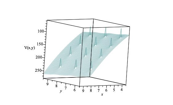
In figure 1 we present a plot of this function for a generic rectangular lattice and for the particular case of a square lattice.

Refer to caption — Figure 1: (Colour online) Three-dimensional plot of the “potential function” $V(x,y)$ for the rectangular and square lattices, respectively.

1.2 Triangular lattice

For the triangular lattice we consider $\vec{a}_{1}=a\hat{x}$ and $\vec{a}_{2}=a\cos(\piup/3)\hat{x}+a\sin(\piup/3)\hat{y}$ such that a point of the lattice located at $\vec{R}_{mn}=m\vec{a}_{1}+n\vec{a}_{2}$ will lead to

|\vec{r}-\vec{R}_{mn}|^{2}=(\varphi-\eta)(\bar{\varphi}-\bar{\eta})\,,

(1.16)

where $\varphi$ is given by equation (1.3) and

\eta=\left(m+\mathrm{e}^{\mathrm{i}\piup/3}n\right)a.

(1.17)

Following the steps of the previous section,

$\displaystyle V(x,y)$	$\displaystyle=\lambda\sum_{(m,n)\in\mathbb{Z}^{2}}\ln\left[(\varphi-\eta)(\bar{\varphi}-\bar{\eta})\right]=\lambda\sum_{m=-\infty}^{\infty}\ln\left[(\varphi-ma)(\bar{\varphi}-ma)\right]$
	$\displaystyle+\lambda\sum_{m=-\infty}^{\infty}\sum_{n=1}^{\infty}\ln[(\varphi^{2}-2ma\varphi+m^{2}a^{2}+e^{-i\piup/3}n^{2}a^{2})$
	$\displaystyle\times(\bar{\varphi}^{2}-2ma\bar{\varphi}+m^{2}a^{2}+\mathrm{e}^{\mathrm{i}\piup/3}n^{2}a^{2})].$	(1.18)

The analogue of equation (1.8) is then

$\displaystyle V(x,y)$	$\displaystyle=\frac{\lambda}{2}\sum_{(m,n)\in\mathbb{Z}^{2}}\ln\left(m^{2}a^{2}+\mathrm{e}^{\mathrm{i}\piup/3}n^{2}a^{2}\right)+\frac{\lambda}{2}\sum_{(m,n)\in\mathbb{Z}^{2}}\ln\left(m^{2}a^{2}+\mathrm{e}^{-\mathrm{i}\piup/3}n^{2}a^{2}\right)$
	$\displaystyle+\lambda\sum_{m=-\infty}^{\infty}\ln\left\{ma\frac{\sinh[\piup(\varphi-ma)\mathrm{e}^{\mathrm{i}\piup/6}/a]}{\sinh(\piup m\mathrm{e}^{\mathrm{i}\piup/6})}\right\}$
	$\displaystyle+\lambda\sum_{m=-\infty}^{\infty}\ln\left\{ma\frac{\sinh[\piup(\bar{\varphi}-ma)\mathrm{e}^{-\mathrm{i}\piup/6}/a]}{\sinh(\piup m\mathrm{e}^{-\mathrm{i}\piup/6})}\right\}.$	(1.19)

After discarding the additive constants, the above expression becomes

$\displaystyle V(x,y)$	$\displaystyle=\lambda\ln[\sinh(\piup\varphi\mathrm{e}^{\mathrm{i}\piup/6}/a)\sinh(\piup\bar{\varphi}\mathrm{e}^{-\mathrm{i}\piup/6}/a)]$
	$\displaystyle+\lambda\sum_{m=1}^{\infty}\ln\left\{\frac{\sinh[\piup(\varphi-ma)\mathrm{e}^{\mathrm{i}\piup/6}/a]\sinh[\piup(\varphi+ma)\mathrm{e}^{\mathrm{i}\piup/6}/a]}{\sinh^{2}(\piup m\mathrm{e}^{\mathrm{i}\piup/6})}\right\}$
	$\displaystyle+\lambda\sum_{m=1}^{\infty}\ln\left\{\frac{\sinh[\piup(\bar{\varphi}-ma)\mathrm{e}^{-\mathrm{i}\piup/6}/a]\sinh[\piup(\bar{\varphi}+ma)\mathrm{e}^{-\mathrm{i}\piup/6}/a]}{\sinh^{2}(\piup m\mathrm{e}^{-\mathrm{i}\piup/6})}\right\},$	(1.20)

in analogy with equation (1.9).

In terms of the coordinates $x$ and $y$ , the final expression for the regularized potential is then

\displaystyle V(x,y)=\lambda\ln\left\{\frac{\vartheta_{1}\left[\mathrm{i}\frac{\piup}{a}\left(x+\mathrm{i}y\right)\mathrm{e}^{\mathrm{i}\piup/6},-\mathrm{i}\mathrm{e}^{-\sqrt{3}\piup/2}\right]\cdot\vartheta_{1}\left[\mathrm{i}\frac{\piup}{a}\left(x-\mathrm{i}y\right)\mathrm{e}^{-\mathrm{i}\piup/6},\mathrm{i}\mathrm{e}^{-\sqrt{3}\piup/2}\right]}{\cosh^{2}\left[\frac{\piup}{2a}\left(y-\sqrt{3}x\right)\right]-\cos^{2}\left[\frac{\piup}{2a}\left(x+\sqrt{3}y\right)\right]}\right\}.

(1.21)

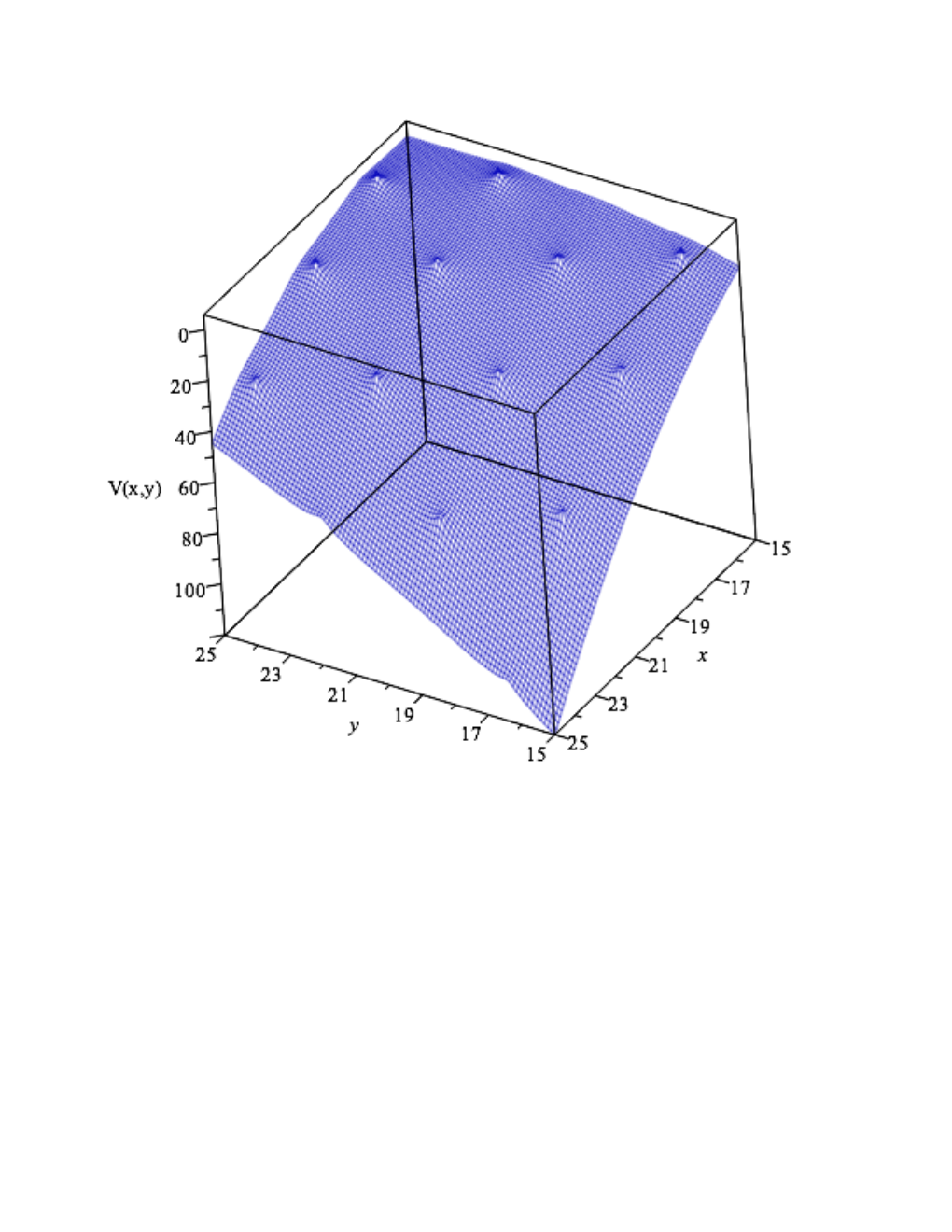
A graphic representation of this function can be seen in figure 2.

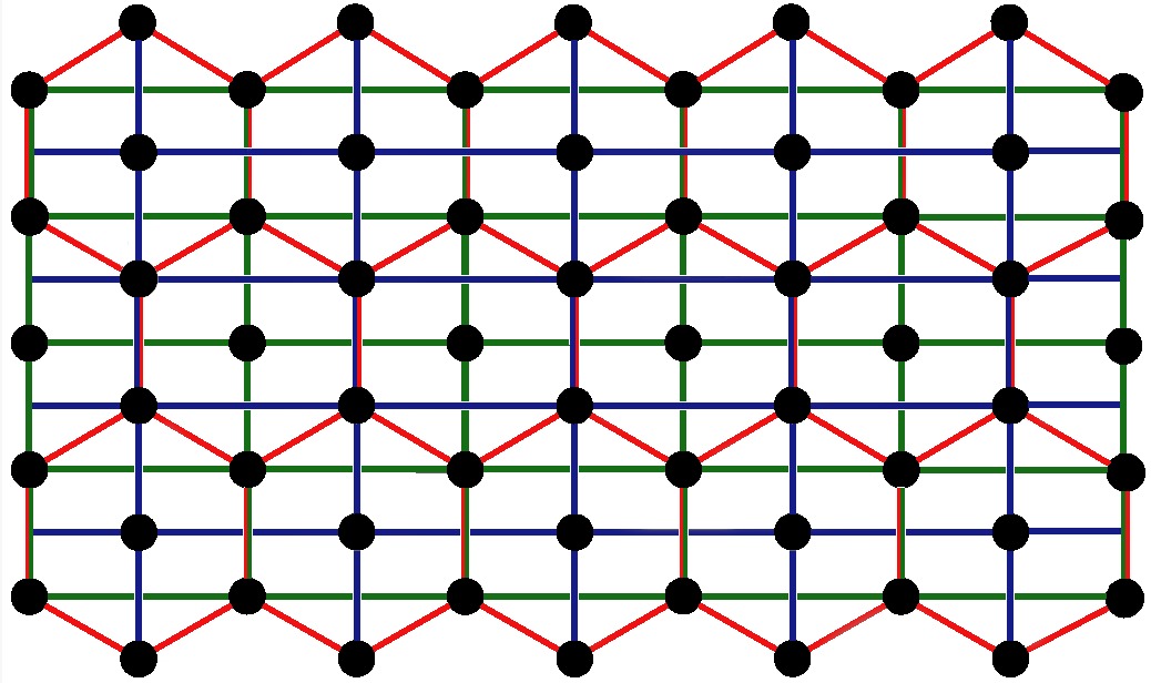
Due to the linearity of equation (1.2), the above result can also be obtained from the superposition of the potentials of two rectangular lattices displaced relatively to each other in such a way as to form the triangular lattice (see figure 3).

2 Conclusion

In this paper, we performed infinite logarithmic sums, with proper regularization, to determine the interaction energy of rectangular and triangular lattices of line defects having their axes along the $z$ -direction. By adjusting the defect strength $\lambda$ , along with parameters governing the geometry of a cell (namely $a$ , $b$ ), one has the possibility to perform defect engineering, that is tailoring material properties from controlled defect arrays [36, 37].

Particles moving inside a lattice of topological defects may be highly sensitive to initial conditions and hence the dynamics of these particles is likely to lead to exponential divergence of initially closed trajectories. The motion of fast electrons in a silicon crystal endowed with periodically distributed atomic strings is known to be chaotic [38] and deserves a separate treatment involving the statistical tools of dynamic hamiltonian systems. This will be the object of a next study.

Acknowledgements

F.M. is thankful for the financial support and warm hospitality of the Statistical Physics Group at Université de Lorraine. This work was partially funded by INCT nanocarbono, CNPq, CAPES and FACEPE (Brazilian agencies) and PICS CNRS (France). We also thank Eudes Gomes for helping with figure 3.

References

[1] Chen J., Chung T.C., Moraes F., Heeger A., Solid State Commun., 1985, 53, No. 9, 757–763,
doi:10.1016/0038-1098(85)90214-5
[2] Kosevich A., Low Temp. Phys., 2004, 30, No. 3, 247–252, doi:10.1063/1.1645186
[3] Lounasmaa O.V., Thuneberg E., PNAS, 1999, 96, No. 14, 7760–7767, doi:10.1073/pnas.96.14.7760
[4] Adhikari S., J. Phys.: Condens. Matter, 2019, 31, No. 27, 275401, doi:10.1088/1361-648x/ab14c5
[5] Abrikosov A.A., Sov. Phys. JETP, 1957, 5, 1174–1182.
[6] Murray B.S., Pelcovits R.A., Rosenblatt C., Phys. Rev. E, 2014, 90, No. 5, 052501,
doi:10.1103/physreve.90.052501
[7] Renn S.R., Lubensky T.C., Phys. Rev. A, 1988, 38, No. 4, 2132, doi:10.1103/physreva.38.2132
[8] Bahr C., Kitzerow H.S., Chirality in Liquid Crystals, Springer, New York, 2001.
[9] Fukuda J.i., Žumer S., Nat. Commun., 2011, 2, 246, doi:10.1038/ncomms1250
[10] Ackerman P.J., van de Lagemaat J., Smalyukh I.I., Nat. Commun., 2015, 6, 6012, doi:10.1038/ncomms7012
[11] Duzgun A., Selinger J.V., Saxena A., Phys. Rev. E, 2018, 97, No. 6, 062706, doi:10.1103/physreve.97.062706
[12] Tai J.S.B., Smalyukh I.I., Science, 2019, 365, No. 6460, 1449–1453, doi:10.1126/science.aay1638
[13] Mazur D., Heyl J.S., Phys. Rev. D, 2015, 91, No. 6, 065019, doi:10.1103/physrevd.91.065019
[14] Bucher M., Spergel D., Phys. Rev. D, 1999, 60, No. 4, 043505, doi:10.1103/physrevd.60.043505
[15] Battye R.A., Chachoua E., Moss A., Phys. Rev. D, 2006, 73, No. 12, 123528, doi:10.1103/physrevd.73.123528
[16] Kibble T.W., J. Phys. A: Math. Gen., 1976, 9, No. 8, 1387, doi:10.1088/0305-4470/9/8/029
[17] Zurek W.H., Nature, 1985, 317, No. 6037, 505, doi:10.1038/317505a0
[18] Bowick M., Chandar L., Schiff E., Srivastava A., Science, 1994, 263, No. 5149, 943–945,
doi:10.1126/science.263.5149.943
[19] Grønbech-Jensen N., Int. J. Mod. Phys. C, 1996, 7, No. 06, 873–881, doi:10.1142/s0129183196000727
[20] Grønbech-Jensen N., Comput. Phys. Commun., 1999, 119, No. 2–3, 115–121,
doi:10.1016/S0010-4655(99)00200-3.
[21] Berezinskii V.L., Sov. Phys. JETP, 1971, 32, 493.
[22] Kosterlitz J.M., Thouless D.J., J. Phys. C: Solid State Phys., 1972, 5, No. 11, L124,
doi:10.1088/0022-3719/5/11/002
[23] Kosterlitz J.M., J. Phys. C: Solid State Phys., 1974, 7, No. 6, 1046, doi:10.1088/0022-3719/7/6/005
[24] Kosterlitz J.M., J. Phys.: Condens. Matter, 2016, 28, No. 48, 481001, doi:10.1088/0953-8984/28/48/481001
[25] Berche B., J. Phys. A: Math. Gen., 2003, 36, No. 3, 585, doi:10.1088/0305-4470/36/3/301
[26] Lavrentiev M., Chabat B., Méthodes de la Théorie des Fonctions d’une Variable Complexe, Mir, Moscou, 1972, (in French).
[27] Di Francesco P., Mathieu P., Sénéchal D., Conformal Field Theory, Springer, New York, 1997.
[28] Talapov A., Andreichenko V., Dotsenko V., Shchur L., Int. J. Mod. Phys. C, 1993, 4, 787–804,
doi:10.1142/s0129183193000653
[29] Chatelain C., Berche B., Phys. Rev. E, 1999, 60, 3853–3865, doi:10.1103/PhysRevE.60.3853.
[30] Glasser M., J. Math. Phys., 1974, 15, No. 2, 188–189, doi:https://doi.org/10.1063/1.1666619
[31] Stremler M.A., J. Math. Phys., 2004, 45, No. 9, 3584–3589, doi:10.1063/1.1777403
[32] Tyagi S., Phys. Rev. E, 2004, 70, No. 6, 066703, doi:10.1103/physreve.70.066703
[33] Tyagi S., Mol. Phys., 2006, 104, No. 3, 359–363, doi:10.1080/00268970500358735.
[34] Abramovitz M., Stegun I.A. (Eds.), Handbook of Mathematical Functions with Formulas, Graphs, and Mathematical Tables, National Bureau of Standards Applied Mathematics Series, Vol. 55, U.S. Government Printing Office, Washington, D.C., 1964.
[35] Olver F.W., NIST Handbook of Mathematical Functions Hardback and CD-ROM, Cambridge University Press, Cambridge, 2010.
[36] Fumeron S., Berche B., Moraes F., Santos F.A.N., Pereira E., Eur. Phys. J. B, 2017, 90, No. 5, 95,
doi:10.1140/epjb/e2017-70384-5.
[37] Santos F., Fumeron S., Berche B., Moraes F., Nanotechnology, 2016, 27, No. 13, 135302,
doi:10.1088/0957-4484/27/13/135302
[38] Akhiezer A., Truten’ V., Shul’ga N., Phys. Rep., 1991, 203, No. 5, 289–343,
doi:10.1016/0370-1573(91)90005-7

Ñòîñîâíî åíåðã¿ ãðàòîê ç òîïîëîãчíèìè äåôåêòàìè Á. Áåðø ${}^{\textsf{\footnotesize{\mbox{?}}}}$ , Ñ. Ôóìåðîí ${}^{\textsf{\footnotesize{\mbox{?}}}}$ , Ô. Ìîðàåñ ${}^{\textsf{\footnotesize{\mbox{?}}}}$

${}^{\textsf{\footnotesize 1}}$

Äèíàìêà ñèìåòðÿ, ëàáîðàòîðÿ ôçèêè òåîðåòèчíî¿ õì¿, CNRS - óíâåðñèòåò Ëîððåí, UMR 7019, Âàíäóâð ë Íàíñ, Ôðàíöÿ
${}^{\textsf{\footnotesize 2}}$

Êàôåäðà ôçèêè, Ôåäåðàëüíèé óíâåðñèòåò Ïåðíàìáóêó 52171–900 Ðåñô, Áðàçèëÿ