Probing the thermal state of the intergalactic medium at with the transmission spikes in high-resolution Ly forest spectra2015Probing the thermal state of the intergalactic medium at with the transmission spikes in high-resolution Ly forest spectra–4
Abstract
We compare a sample of five high-resolution, high S/N Ly forest spectra of bright QSOs aimed at spectrally resolving the last remaining transmission spikes at with those obtained from mock absorption spectra from the Sherwood and Sherwood-Relics suites of hydrodynamical simulations of the intergalactic medium (IGM). We use a profile fitting procedure for the inverted transmitted flux, , similar to the widely used Voigt profile fitting of the transmitted flux at lower redshifts, to characterise the transmission spikes that probe predominately underdense regions of the IGM. We are able to reproduce the width and height distributions of the transmission spikes, both with optically thin simulations of the post-reionization Universe using a homogeneous UV background and full radiative transfer simulations of a late reionization model. We find that the width of the fitted components of the simulated transmission spikes is very sensitive to the instantaneous temperature of the reionized IGM. The internal structures of the spikes are more prominent in low temperature models of the IGM. The width distribution of the observed transmission spikes, which require high spectral resolution ( 8 km s-1) to be resolved, is reproduced for optically thin simulations with a temperature at mean density of K at . This is weakly dependent on the slope of the temperature-density relation, which is favored to be moderately steeper than isothermal. In the inhomogeneous, late reionization, full radiative transfer simulations where islands of neutral hydrogen persist to , the width distribution of the observed transmission spikes is consistent with the range of caused by spatial fluctuations in the temperature-density relation.
Keywords:
cosmology: large-scale structure of Universe - methods: numerical - galaxies: intergalactic medium - QSOs: absorption lines1 Introduction
The reionization of intergalactic H i and He i by ultraviolet photons from stars and black holes in the first galaxies is one of the major phase transitions of the universe (Fan et al. 2001; Fan et al. 2006; Robertson et al. 2010; Bolton et al. 2011; Planck Collaboration et al. 2014; Planck Collaboration et al. 2018). Photo-heating during the reionization increases the temperature of the intergalactic medium (IGM) (Hui & Gnedin 1997; Trac et al. 2008; McQuinn et al. 2009; McQuinn & Upton Sanderbeck 2016). The thermal and ionization histories of the Universe are thus interlinked, and can be used in tandem to understand the process of reionization and the nature of ionizing sources (Haehnelt & Steinmetz 1998; Furlanetto & Oh 2009; McQuinn et al. 2011; Becker et al. 2015; Chardin et al. 2017; Davies et al. 2018; Keating et al. 2018; Kulkarni et al. 2019b).
The H i Ly forest observed along sightlines towards bright QSOs is frequently used to constrain the thermal and ionization state of the IGM at . For underdense or moderately overdense regions, the thermal state of the IGM is often approximated as a power law, parameterized as the temperature at mean density and the slope of the power law (Lidz et al. 2010; Becker et al. 2011; Rudie et al. 2012; Garzilli et al. 2012; Bolton et al. 2014; Boera et al. 2014; Hiss et al. 2018; Telikova et al. 2018; Telikova et al. 2019; Walther et al. 2019; Boera et al. 2019, and ). Other relevant parameters are the H i photo-ionization rate (Rauch et al. 1997; Bolton & Haehnelt 2007; Faucher-Giguère et al. 2008; Calverley et al. 2011; Becker & Bolton 2013; Gaikwad et al. 2017a; Gaikwad et al. 2017b; Viel et al. 2017; Khaire et al. 2019, ) and the pressure smoothing scale (Gnedin & Hui 1998; Peeples et al. 2010; Kulkarni et al. 2015; Lukić et al. 2015; Rorai et al. 2017a). Due to the rapid increase of the Ly opacity with redshift, the transmitted Ly flux at is close to zero, with the occurrence of a few transmission spikes indicating that the reionization process is inhomogeneous (Becker et al. 2015; Bosman et al. 2018; Eilers et al. 2018). Analysis of the transmission spikes towards ULAS J1120+0641 QSO (Becker et al. 2015; Barnett et al. 2017, ,) with numerical simulations suggests that these spikes correspond to underdense, highly ionized regions of gas (Gnedin et al. 2017; Chardin et al. 2018; Kakiichi et al. 2018; Garaldi et al. 2019; Nasir & D’Aloisio 2019). These studies find that the number and height of the spikes are sensitive to the ionization fraction ( ) of the IGM, which in turn depends on the photo-ionization rate and the temperature of the gas in the ionized regions. Perhaps somewhat surprisingly, however, Garaldi et al. 2019 found that the spike shape (especially the widths of the spikes) appeared to be only weakly correlated with the temperature of the IGM. We revisit this question here with a larger sample of higher resolution, higher quality Ly forest spectra which we compare to high-resolution hydrodynamical simulations of the IGM using the Sherwood and Sherwood-Relics simulation suites. These incorporate simulations with a homogeneous UV background as well as full radiative transfer simulations of inhomogeneous reionization (Bolton et al. 2017; Kulkarni et al. 2019b, Puchwein et.al. 2020 in prep). Note that in the main analysis we used the Sherwood-Relics simulation suite, but complemented these with simulations from the Sherwood simulation suite for additional tests performed in the Appendices.
There are several difficulties in probing the effect of the thermal state of the IGM on Ly transmission spikes. High-redshift QSOs, while intrinsically luminous, are nevertheless faint and observed spectra are normally taken at moderate resolution as e.g. offered by VLT/X-Shooter, i.e. with km s-1 or worse. As a result most spectra of high-redshift transmission spikes are of rather modest quality and the number of well observed transmission spikes is necessarily still small due to the rarity and faintness of high- background QSOs (Kulkarni et al. 2019a). We improve this situation here and present a sample of 5 high resolution ( km s-1) and high S/N () QSO absorption spectra obtained using the Magellan Inamori Kyocera Echelle (MIKE) spectrograph on the Magellan II telescope (Bernstein et al. 2003), and the High-Resolution Echelle Spectrograph (HIRES) on the Keck I telescope (Vogt et al. 1994).
Similarly, simulated transmission spikes may be drawn from simulations with moderate mass or spatial resolution that is only sufficient to produce mock spectra mimicking moderate resolution spectrographs like X-Shooter (Garaldi et al. 2019, km s-1, but see). The thermal smoothing scale of the Ly transmitted flux due to the IGM temperature ( km s-1) is, however, significantly smaller than this. As discussed in detail by Bolton & Becker 2009, rather high mass or spatial resolution is required to resolve the small scale structure in the underdense regions of the IGM probed by Ly forest spectra at high redshift. Previous theoretical work has focused on analyzing the spikes in radiative transfer simulations (Gnedin et al. 2017; Chardin et al. 2018; Garaldi et al. 2019). While these simulations are physically well motivated, they are computationally expensive and it is hard to disentangle the effect of the thermal state of the IGM on the transmission spikes from the reionization history and numerical limitations.
We have thus chosen to analyze the transmission spikes first in very high resolution, high dynamic range optically thin simulations with different thermal and reionization histories where a single parameter is varied at a time while keeping other parameters fixed. We therefore use simulations from the Sherwood and Sherwood-Relics simulation suite (Bolton et al. 2017, Puchwein et.al. 2020 in prep) to show how spike properties depend on the IGM thermal state, the H i photo-ionization rate , and (in the appendices) the pressure smoothing scale, as well as the mass resolution and box size of the simulations. Once we have established this we investigate the effect of inhomogeneous reionization in more physically motivated, spatially inhomogeneous H i reionization simulations including radiative transfer (Kulkarni et al. 2019b; Keating et al. 2019, see).
Another problem when comparing simulated and observed Ly forest spectra is the accurate characterisation of the transmission spike properties. Transmission spikes are often asymmetric and transmission features appear “blended”. The often used simple definition of height and width of spikes based on the maximum and FWHM of the transmitted flux will thus not capture the detailed information contained in the complex spike shapes, and could be the reason that the analyses performed so far show little or no correlations with astrophysical parameters (Garaldi et al. 2019, see e.g. the width vs temperature correlation in). Characterizing the shape of transmission spikes becomes even more crucial for high S/N, high resolution QSO absorption spectra. In practice the problem is very similar to that of the characterisation of Ly absorption lines at lower redshift. To utilise the practical experience gained in this area with existing software packages (Gaikwad et al. 2017b, e.g.) we characterize the transmission spikes by fitting Voigt profiles to the “inverted” transmitted flux, . We will later show that the fitted parameters obtained in this way are well correlated with physical properties (e.g. the density and temperature) of the gas associated with the transmission spikes. We will also study how the statistics of the fitted parameters depend on the astrophysical parameters , and . Unlike for absorption lines, there is no direct physical motivation for fitting Voigt profiles to 1-F, so this should be considered as a purely heuristic approach to comparing simulated and observed spectra. However, as we will see this does not mean that the fit parameters obtained do not correlate with physical properties.
The main goal of this paper is to constrain the thermal state of the IGM at . The paper is organized as follows: In §2 we present the high resolution spectra of 5 QSOs and discuss qualitatively the physical origin of Ly transmission spikes. We present the properties of transmission spikes in optically thin simulations in §3 and §4. We demonstrate the sensitivity of spike statistics to the IGM thermal state in §5. The main results of the paper are presented in §5.3 and §6 by comparing the observed spike statistics with those from optically thin and radiative transfer simulations. We summarize our findings in §7. We assume a flat cosmological model consistent with Planck Collaboration et al. 2014; Planck Collaboration et al. 2018. All distances are given in comoving units unless specified. expressed in units of is denoted by .
2 Transmission spikes in high-resolution, high-redshift Ly forest spectra
2.1 Observations: high-resolution spectra of transmission spikes
The data consist of the high resolution echelle spectra of five recently discovered QSOs. The objects were chosen for their brightness, and individual targets were further selected to maximize the exposure time during a given observing run. Table 1 gives the name of each object, the emission redshift zem, the J AB band magnitude (Ross & Cross 2019, from the compilation of), the total on-source exposure time T in hours, and a typical signal-to-noise ratio per pixel. The objects were observed under mostly photometric conditions in sub-arcsec seeing. The first four objects were observed with the MIKE instrument (Bernstein et al. 2003) on the Magellan II telescope at Las Campanas Observatory. A 0.5” wide slit gave a measured spectral resolution of 5 km s-1 (FWHM). The spectra were binned onto 2 km s-1 wide pixels. The spectrum of SDSSJ010013.02+280225.8 was obtained with the HIRES instrument (Vogt et al. 1994) on the Keck I telescope, and a 0.861” wide slit, giving a resolution of 6.1 km s-1 (FWHM), sampled by 2.5 km s-1 wide bins. The data were reduced with a custom pipeline (Becker et al. 2012). Optimal sky-subtraction on the individual, un-rectified exposures was performed according to the prescription by Kelson 2003.
For the continuum model, a power law was assumed. As the high resolution echelle spectra only had limited coverage of the unabsorbed region redward of the Ly emission, the continuum was derived from flux-calibrated, low resolution spectra of the same QSOs which extended further to the red. For objects 1-3 (in table 1), the continua were determined from the discovery spectra, using fits to regions redward of Ly avoiding broad emission lines, whereas the power law slopes for objects 4 and 5 were taken from the literature cited. The continuum was then scaled uniformly to match the flux-calibrated high resolution spectrum in the overlap region with the low-resolution spectrum redward of Ly, and divided into the spectrum. To correct for the rapidly variable region of the spectrum near the Ly emission line, the emission line region was fitted with a higher order polynomial in the previously continuum divided spectrum, which then was multiplied into the previous continuum fit. The final continuum thus obtained was divided into the data. As we show later, the width of the fitted components of the transmission spikes are relatively robust to continuum fitting uncertainty.
During data reduction a certain degree of smoothing is introduced into the data that appears as a discrepancy between the RMS fluctuations in the final data and the propagated error array, and generally results in an underestimate of the reduced when fitting line profiles. To counteract this problem, a correction factor (generally a number close to unity varying slowly with wavelength) was derived from the observed ratio between the RMS fluctuations and the error array, as determined from wavelength windows in the spectrum with zero flux. A linear fit to the correction factor as a function of wavelength was divided into the error array to obtain a reduced during profile fitting.
| ID | Name | J | (S/N)/pixel | Reference | Instrument | Dates of the observations | ||
|---|---|---|---|---|---|---|---|---|
| 1 | ATLASJ158.6938-14.4211 | 6.07 | 19.27 | 11.8 | 7.7 | Chehade et al. 2018 | MIKE | March and April, 2018 |
| 2 | PSOJ239.7124-07.4026 | 6.11 | 19.37 | 10.0 | 6.5 | Bañados et al. 2016 | MIKE | March, April and June, 2018 |
| 3 | ATLASJ025.6821-33.4627 | 6.34 | 19.10 | 6.7 | 12.0 | Carnall et al. 2015 | MIKE | October and December, 2018 |
| 4 | J043947.08+163415.7 | 6.51 | 17.47 | 10.0 | 30.3 | Fan et al. 2019 | MIKE | October and December, 2018 |
| 5 | SDSSJ010013.02+280225.8 | 6.30 | 17.60 | 5.0 | 20.0 | Wu et al. 2015 | HIRES | November 2017 |
2.2 Characterising width and height of individual components
Fig. 1 compares transmission spikes in a high-resolution Ly forest observation of the QSO J043947.08+163415.7 with the MIKE spectrograph with simulated spikes drawn from the Sherwood-Relics simulation suite (see Section 3.1, Puchwein et.al. 2020 in prep), for cold and hot models with a spatially uniform UV background. The transmission spikes have complex shapes composed of many asymmetric and blended features. Even isolated transmission spikes are often highly asymmetric and consist of two or more “components”. In order to facilitate a more quantitative discussion of the transmission spikes, we focus on two properties, namely the height and width of individually identifiable components. We quantify these (see §4) by fitting the “inverted” transmitted flux, , with multi-component Voigt profiles, similar to the fitting of Voigt profiles of the transmitted flux, , often employed at lower redshift to characterise absorption lines.
The best fits to observed and simulated spectra are shown in Fig. 1 by the red curve. The location of individual identified components are marked by black vertical lines. Fig. 1 show simulated spectra for the hot and cold model and illustrate the sensitivity of spike features to the thermal state of the IGM. The main effect of increase in IGM temperature is to reduce the internal structure of the spikes (i.e., more blending). As a result, fewer and broader components are required to fit the transmission spikes in the hot model. In general, the spikes in the hot model are (i) broader, (ii) larger in height, (iii) more asymmetric and (iv) more blended (hence fewer in number) than those in the corresponding cold model. It is interesting to note that the number and shape of the spikes in the hot model are qualitatively very similar to those in the observed spectra. We will analyse this more quantitatively below.
2.3 The origins of transmission spikes
The complex shapes of the transmission spikes shown in the last section will be a superposition of features in the line-of-sight distribution of density, temperature, photo-ionization rate and peculiar velocity. To get a better feel for this in Fig. 2 we show mock spectra where we isolate the effect of varying these parameters, one at a time. Fig. 2 illustrates how the variation in any of these physical quantities along a sightline can lead to regions of smaller H i optical depth and hence transmission spikes. Panels A1-A6, B1-B6 and C1-C6 show the effect of underdensity, enhanced and enhanced temperature along a sightline, respectively. All these effects can result in a smaller number density of neutral hydrogen, , along the sightline. Panels D1-D6 show that a diverging peculiar velocity field along the sightline can also produce transmission spikes. Hot, ionized underdense regions subjected to high photo-ionization rates and diverging peculiar velocities will thus produce the most prominent transmission spikes in high QSO absorption spectra (Gnedin et al. 2017; Chardin et al. 2018; Garaldi et al. 2019). The transmission spikes shown in Fig. 2 are by construction isolated, symmetric and simple. As discussed in the previous section, transmission spikes in both observed spectra and spectra drawn from cosmological hydrodynamical simulations have complicated shapes, as generally more than one of the above effects contribute.
3 Transmission spikes in optically thin simulations
3.1 The Sherwood and Sherwood-Relics simulation suites
We use cosmological hydrodynamical simulations from the Sherwood-Relics simulation suite to investigate transmission spikes in the high-redshift Ly forest; see Table 2 for an overview. The simulations were performed with a modified version of the p-gadget-3 code (itself an updated version of the gadget-2 code presented in Springel 2005). The code uses a tree-particle mesh gravity solver for following cosmic structure formation and a manifestly energy and entropy-conserving smoothed particle hydrodynamics scheme (Springel & Hernquist 2002) for following the hydrodynamics. The Sherwood-Relics simulations build upon the original Sherwood simulation suite (which is used in Appendix C to study numerical convergence) in that the initial conditions were generated in the same way, and much of the modeling of the IGM and Ly forest is based on similar methods (Bolton et al. 2017)11 1 https://www.nottingham.ac.uk/astronomy/sherwood/.
Our main production runs follow particles in a volume, corresponding to a gas mass resolution of . For the gravitational softening we adopt . Star formation is treated with a rather simplistic but numerically efficient scheme in which all gas particles with densities larger than 1000 times the mean cosmic baryon density and temperatures smaller than K are converted to collisionless star particles. While this does not produce realistic galaxies, it allows robust predictions of the properties of the IGM (Viel et al. 2004a). Photo-heating and photo-ionization are followed based on external UV background models. In a departure from the Sherwood simulations, we use a non-equilibrium ionization and cooling/heating solver (Puchwein et al. 2015; Gaikwad et al. 2019) for following the thermochemistry of hydrogen and helium. This ensures that no artificial delay between the reionization of gas and its photo-heating is present. We have also replaced the slightly modified Haardt & Madau 2012 UV background used in Sherwood with the fiducial UV background model from Puchwein et al. 2019 in our default run. This results in a more realistic reionization history with hydrogen reionization finishing at . The cold/hot models were obtained by decreasing/increasing the H i and He i photo-heating rates in the fiducial UV background model by a factor of 2 and the He ii photo-heating rate by a factor of , while keeping all photo-ionization rates fixed. Mock Ly forest spectra were extracted from all simulations as described in Bolton et al. 2017 (Gaikwad et al. 2018; Gaikwad et al. 2019, see also). Through out this work, we use simulations from the Sherwood-Relics simulation suite for the main analysis. Additional simulations from the Sherwood simulation suite are used for convergence tests as described in Appendix C.
3.2 The temperature density relation (TDR) in optically thin simulations

| Fraction of spikes (in per cent) showing the effect of | ||||
| Simulation | Underdensity[a] | Enhanced [b] | Enhanced [c] | Peculiar velocity[d] |
| L40N2048_DEFAULT [e] | 89.1 | 5.7 | 18.8 | |
| L40N2048_COLD [e] | 89.3 | 4.9 | 14.8 | |
| L40N2048_HOT [e] | 89.8 | 5.5 | 19.9 | |
| L40N2048_ATON | 84.4 | 56.8 | 50.1 | 19.5 |
| L40N2048_PATCHY | 79.2 | 54.7 | 40.3 | 18.4 |
- a
Fraction of all spikes with .
- b
Fraction of all spikes with where is the optical depth weighted median calculated from all the sightlines (i.e., regions with and without spikes).
- c
Fraction of all spikes with where is the optical depth weighted median temperature calculated from all the sightlines (i.e., regions with and without spikes).
- d
Fraction of all spikes with km s-1 where is difference between mean velocity on redward and blueward side of spike center. For diverging velocity flow , whereas for converging velocity flow . The limit of km s-1 corresponds to the spectral resolution of the instrument.
- e
L40N2048_DEFAULT L40N2048_COLD and L40N2048_HOT are optically thin simulations that do not include fluctuations in .
Fig. 3 shows the TDR in the hot and cold models of the Sherwood-Relics simulation suite. We shall compare the hot and cold models to study the effect of temperature on transmission spikes. Note that the hot model is not only hotter than the cold and the default model but also has a flatter temperature density relation, and that the ionization state of the gas is also different in the models. This is because the recombination coefficient is temperature dependent. For the same photo-ionization rate the H i fraction is therefore smaller in the hot model. The models aton and patchy incorporate the effect of inhomogeneous UV background that we describe in 6.
3.3 Examples of transmission spikes in the hot and cold optically thin simulations
Fig. 4 shows the relevant physical properties along the two sightlines in the hot and cold models. As expected, the hot model shows (i) a smoother density () field in real space, (ii) a smaller H i fraction ( ), (iii) a larger temperature () and (iv) a smoother velocity () field compared to the corresponding cold model. The smoothing of the real-space density field and the velocity field can be attributed to the increased effect of pressure smoothing in the hot model. The resultant Ly optical depth and transmitted flux calculated from the , , and fields are shown in panels A6-B6 and panels A7-B7, respectively. Note that the location of spikes in the green and yellow shaded regions in redshift space differs in real space due to the effect of peculiar velocities. The transmission spikes in the hot and cold models have complicated shapes, qualitatively similar to that in the observed spectra (Fig. 1). The smoother transmission features in the simulated spectra of the hot model are more similar to those in the observed spectra than those in the more “spiky” spectra in the cold model.
In both models, the transmission spikes correspond to regions of low H i optical depth ( , black dashed line). The peaks in transmission are well correlated with those in the optical depth weighted overdensities ( ).22 2 accounts for the redshift space effect of peculiar velocity on . To assign a single overdensity/temperature to each transmission spike, we calculate flux weighted overdensity/temperature (Garaldi et al. 2019, also see). It is clear from Fig. 4 that the spikes in the hot model are smoother, broader and more prominent than in the cold model. Furthermore the number of individual transmission components is significantly smaller in the hot model than in the cold model due to the “thermal blending” of transmission features. The shape and number of transmission spikes in our simulated spectra are clearly sensitive to the thermal and ionization state of the IGM in a manner that we will quantitatively discuss below.
Table 2 shows the physical effects responsible for the occurrence of transmission spikes in the optically thin hot and cold simulations. Most of the spikes ( percent) in the hot and cold models occur in underdense regions. Around percent of spikes show a diverging velocity field along the sightline. The effect of enhanced temperature on the occurrence of transmission spikes is marginal in both hot and cold optically thin simulations.
In summary, Fig. 4 and Table 2 show that underdense ( ), more highly ionized (minimum in ) and hotter regions along a sightline produce more prominent spikes. This motivates us to quantify the shape of spikes and to introduce statistics that are sensitive to the thermal and ionization parameters of the IGM.
4 Characterising the properties of transmission spikes in optically thin simulations
4.1 Voigt profile fitting of the inverted flux
The shape of absorption features is usually characterized by Voigt profiles defined by three parameters: (i) the centre of absorption lines (), (ii) the H i column density () and (iii) the width of the absorption () features. Most of the absorption features in the high- Ly forest are saturated () and strongly blended. It is well known that Voigt profile decompositions are highly degenerate for saturated lines and very sensitive to systematic errors due to continuum fitting and treatment of noise properties (Webb & Carswell 1991; Fernández-Soto et al. 1996). The inverted transmitted flux, , however, becomes similar in appearance to the absorption features in the Ly forest at lower redshift, where Voigt profile fitting is much less problematic. For convenience, we have thus fitted Voigt profiles to , building on existing experience with Voigt profile decomposition of complex blended spectral profiles. At the redshift we consider here the transmission spikes are observed to be unsaturated, so effectively we use our VoIgt profile Parameter Estimation Routine (Gaikwad et al. 2017b, viper,) to fit multi-component Voigt profiles to the transmission profiles. Similar to absorption lines, a simple, isolated and symmetric spike is fitted by parameters: (i) a spike centre (), (ii) the logarithm of the pseudo-column density (denoted by ) and (iii) a spike width (). The pseudo-column density is thereby a measure of the deficiency of H i along the sightline where the spike occurs. For example, a larger value of means a large H i deficit hence a more prominent spike. Our measured are sensitive to the H i photo-ionization rate . The interpretation of the other two parameters i.e., and width of the spikes remains unchanged when we fit . As we show below, the distribution of spike widths is sensitive to the thermal state of the IGM and can be used to constrain the temperature of the IGM.33 3 Unlike for absorption lines, there is no direct relation between temperature of the absorbing gas and the width of the spikes, such that .
Our main aim is to use the distribution of spike widths to constrain the thermal state of the IGM. As we will show later, these are much less sensitive to IGM ionization state and continuum fitting uncertainties than the heights of the spikes. Note that we rescale the optical depth in different models to match observations as to account for the uncertainty in at (rescaling is not applied in Fig. 4). We show such rescaling does not significantly affect the widths of the line in Appendix A.
4.2 The physical properties of the gas probed by transmission spikes
4.2.1 The dependence of spike height on density: vs

We now turn to connecting the observed spike shapes to optical depth weighted physical properties of the IGM in the optically thin simulations (Gaikwad et al. 2017a, see Eq. 12 in). In Fig. 5, we show the optical depth weighted overdensity against spike height as measured by (pseudo) column density for the cold and hot models. In both models the corresponding overdensity of spikes is i.e., most of the spikes occur in underdense regions. Note that applying a rescaling of optical depth to correct for the uncertain amplitude of the UV background results in a systematic increase or decrease of . However, the overdensities corresponding to spikes are relatively robust. This is also evident from Fig. 4, where the spikes in the hot and cold models correspond to similar overdensities (rescaling is not applied in Fig. 4).
Fig. 5 also illustrates that and are anti-correlated i.e. a larger spike height and higher H i pseudo-column density corresponds to smaller overdensity . We quantify the degree of anti-correlation by fitting a straight line of the form . The normalisation (0.24 for cold and 0.26 for hot) and slope ( for cold and for hot) of the correlation in the two models are in good agreement with each other. This suggests that the thermal state of the gas does not have a strong effect on the correlation when optical depths are rescaled to match observations. Note, however, that the scatter in for a given (e.g., at ) correlation is smaller in the hot model. This is because the spikes are smoother and hence there is less variation in .
4.2.2 The dependence of spike width on temperature: vs

The widths of the components fitted to the spikes are sensitive to the instantaneous temperature along the sightline (see Fig. 1 and Fig. 4). Fig. 6 shows the correlation of optical depth weighted temperature ( ) with spike width () for the cold and hot model. The range in temperature associated with spikes is small for both models. This is expected as the slope of the TDR (Fig. 3) for both models is relatively flat and the temperature associated with is relatively constant.
Fig. 6 illustrates that the spike widths are well correlated with temperature. The spike widths are systematically larger in the hot model () compared to the cold model (). Even though the range in temperature is small () for both models, the scatter in is relatively large (). In §5.4 we will use the spike width distribution to constrain the temperature of the IGM.
4.2.3 The correlation of spike width and height: vs

The relation of absorption line widths with column density and its relation with the thermal state of the gas at has been widely discussed in the literature (Schaye et al. 1999; Bolton et al. 2014; Gaikwad et al. 2017b; Rorai et al. 2017b; Rorai et al. 2018; Hiss et al. 2018; Hiss et al. 2019). The equivalent relation for the Voigt profile parameters of the transmission spikes in our simulated spectra is compared in Fig. 7 to the observed spectra (white crosses). Fig. 7 shows a strong positive correlation between and for both models. We fit this correlation with a straight line of the form with km s-1) and ) for the hot and cold model, respectively. The hot model is in significantly better agreement with the observations than the cold model. The somewhat flatter slope in the hot model is likely due the flatter TDR in the hot simulation. Note further that the scatter in is slightly larger in the hot model. This is because the spikes are more blended and hence less distinctive (Fig. 1 and Fig. 4). The scatter in is similar.
In summary, we find strong correlations of the Voigt profile parameters with physical quantities in the optically thin simulations, where : (i) the gas probed by the transmission spikes is typically underdense ( and (ii) the spike widths (heights) are strongly (anti-) correlated with temperature (density).
5 Comparing transmission spike properties in observations and simulations
5.1 Characterising the flux distribution in transmission spikes
Constraints on cosmological and astrophysical parameters from Ly forest data have been obtained typically by using either a variety of statistical measures of the Ly transmitted flux and/or Voigt profile decomposition (Storrie-Lombardi et al. 1996; Penton et al. 2000; McDonald et al. 2000; McDonald et al. 2005; Viel et al. 2004b; Viel et al. 2009; Becker et al. 2011; Shull et al. 2012). Here we briefly consider both approaches before focusing on constraints on the thermal state of the IGM from the width distribution of transmission spikes. The transmitted flux based statistics (such as the probability distribution function and power spectrum) are straightforward to derive from simulations and observations. For the Voigt profile parameter based statistics, we have fitted Voigt profiles to the inverted transmitted flux, , using viper 44 4 Note that as the transmission spikes are generally not “saturated” in 1-F, we are effectively fitting Gaussian profiles..
The simulated spectra mimic the observed spectra in terms of S/N and instrumental resolution. viper accounts for these effects when determining the best fit parameters, the statistical uncertainty on best fit parameters and a significance level for each Voigt component. For deriving the spike statistics, we chose only those Voigt components with relative error on parameters and with a significance level . We consider three statistics of the flux distribution in the transmission spikes that are sensitive to astrophysical parameters i.e., , and (for a given cosmology) which are discussed below.
5.2 Statistics of the flux distribution in transmission spikes
5.2.1 Spike width (-parameter) distribution function
For absorption features the line width distribution is frequently used as a diagnostic for the gas temperature, turbulence, and the impact of stellar and AGN feedback on the IGM at (Rauch et al. 1996; Tripp et al. 2008; Oppenheimer & Davé 2009; Muzahid et al. 2012; Viel et al. 2017; Gaikwad et al. 2017a; Nasir et al. 2017). By contrast, the width of the individual spikes is not a direct measure of the temperature of the low density gas (i.e., ). Nevertheless we find that the widths of transmission spike components is systematically larger if the temperature of the IGM is larger. 55 5 Since spikes trace cosmic voids, the spike width distribution could in principle also be sensitive to cosmological parameters e.g., , , and . In this work we used the spike width distribution to constrain the thermal state of IGM for a given cosmology.
5.2.2 Pseudo Column Density Distribution Function (pCDDF)
Similar to the H i column density distribution function (CDDF) at low redshift, we define the pseudo-CDDF (pCDDF) as the number of spikes with a pseudo column density in the range to in the redshift interval to (Schaye et al. 2000; Shull et al. 2012). We calculate the pCDDF in 7 bins centered at with d . This choice of bins is motivated by the S/N and resolution of the observed spectra. The pCDDF characterizes the height and number of spikes in a given redshift bin, and is sensitive to the thermal and ionization parameters of the IGM.
5.2.3 Transmitted flux power spectrum (FPS)
The transmitted flux power spectrum (FPS) is frequently used to constrain cosmological (McDonald et al. 2000; Meiksin & White 2004; Viel et al. 2004b) and astrophysical parameters (Walther et al. 2019; Boera et al. 2019, especially parameters describing the thermal state;). The FPS is a measure of the clustering of the pixels in transmission spikes. One can also study the two point correlation of spikes (Maitra et al. 2019, see e.g., ). However, due to the limited number of observed QSOs and the smaller number of spikes detected per sightline, the two point correlation function of spikes is rather noisy. It is important to note that, unlike the pCDDF or the spike width distribution, the FPS is a transmitted flux based statistic that does not require us to fit the spikes. The FPS can, however, only be reliably estimated for a limited range of scales because of finite length of the spectra and other systematic effects. The smallest (larger scales) modes are limited by the length of the simulation box and continuum fitting uncertainties of the observed spectra. The largest modes (smallest scales) on the other hand are limited by the resolution of the instrument and the noise properties (S/N and noise correlation scale if non-Gaussian) of the observed spectra. To account for this, we calculate the FPS in the range with bin width (Kim et al. 2004)66 6 The smallest mode corresponds to a scale of cMpc..
5.2.4 Error estimation
We estimate the error for the spike and flux statistics from the simulation using an approach similar to that in Rollinde et al. 2013 and Gaikwad et al. 2018. For this, we generate samples of 5 simulated Ly forest spectra corresponding to 5 observed QSO spectra with the same observational property i.e., redshift path length, noise property, number of pixels etc. A collection of 5 spectra constitutes a single mock sample. We generate 80 such mock sample and compute the covariance matrix for each statistics. We find that the covariance matrix is converged and dominated by diagonal terms for all the statistics.
We have also estimated the covariance matrix from observations using a bootstrap method. Here we find that the off-diagonal terms of the covariance matrix estimated with the bootstrap method are not converged. The bootstrap method (diagonal terms) underestimates the error by percent as compared to those estimated from the simulations. Throughout this work, we use bootstrap errors increased by a corresponding factor for each statistics.
5.3 Transmission spike statistics: optically thin simulations vs observations
Fig. 8 compares the spike width distribution, pCDDF and FPS from observations with that of the optically thin simulations for three different redshift bins centered at .77 7 The mean transmitted flux in hot, cold and default models is matched to that in the observed spectra to account for the uncertainty in the continuum placement and UV background amplitude, see appendix A. The corresponding residuals suggest a good level of agreement between the default model and observations for all three statistics. The residuals for the hot model with K and are somewhat larger. Overall the three statistics for the default and hot model are in noticeably better agreement than those for the cold model, with differences in the Doppler parameter distribution being most pronounced where agreement with the default model is significant better than with both the hot and cold model. The cold model also predicts more power on small scales, as well as a larger number of spikes with small than observed, and is clearly the model that is least consistent with the observations. We further quantify the degree of agreement between models and observation in appendix D.
5.4 Constraining thermal parameters with optically thin simulations
In the optically thin simulations there is a well defined TDR in underdense and moderately overdense regions. It is thus common practice to study the effect of the thermal state on flux statistics by imposing different TDRs by rescaling temperatures (Hui & Gnedin 1997; Rorai et al. 2017b; Rorai et al. 2018). In Appendix B we use such rescaling to show how the three flux statistics we consider here depend on thermal parameters and and the photo-ionization rate, and demonstrate that it is the width distribution of the transmission spikes which is most sensitive to the thermal state of the gas. We further show that, for the reionization and thermal history models we consider in this work, the spike statistics are only very weakly affected by pressure (Jeans) smoothing at the typical gas densities probed by the Ly transmission spikes (Gnedin & Hui 1998; Theuns et al. 2000; Peeples et al. 2010; Kulkarni et al. 2015; Lukić et al. 2015; Nasir et al. 2016; Maitra et al. 2019; Wu et al. 2019).
We use the spike width distribution to obtain an estimate of the best fit values and uncertainty for the thermal parameters 88 8 We find that the FPS and pCDDF statistics are sensitive to continuum fitting uncertainty and , whereas the spike width distribution is less sensitive to continuum placement and (see Appendix A). We vary and by assuming a TDR of the form for and for . We use the and fields from the optically thin default model, which falls in between the cold and hot models. We vary between to in steps of and between to in steps of . For each model we (i) compute the Ly transmitted flux, (ii) post-process the transmitted flux to match observations, (iii) fit the inverted transmitted flux with Voigt profiles and (iv) compute spike statistics. We use 2000 sightlines for each model. Fig. 9 shows the constraints on in three redshift bins.99 9 To a good approximation, the likelihood function is Gaussian distributed on grids. See Appendix C for details. Fig. 9 also shows the marginal distributions of and . Table 3 summarizes the best fit values and uncertainty on and values under the assumption that the IGM is optically thin. The uncertainty on the and measurement accounts for the uncertainty due to continuum fitting, mean flux and Jeans smoothing effects (see Appendix A and B). The best fit values and uncertainty on and are consistent with each other within for the three redshift bins. As the spikes are probing predominantly gas at densities lower than the mean, the inferred values for and are strongly correlated. We will come back to this in Appendix B.
Fig. 10 compares the evolution of and from this work with a variety of measurements in the literature (Becker et al. 2011; Bolton et al. 2012; Bolton et al. 2014; Boera et al. 2014; Rorai et al. 2017b; Hiss et al. 2018; Walther et al. 2019; Boera et al. 2019). 1010 10 Bolton et al. 2012 measure in QSO proximity regions at . Their constraint including (excluding) a model for the He ii photo-heating by the QSOs is shown by green circles (blue squares) in Fig. 10. Theoretical models for the evolution of and from Puchwein et al. 2019 and Haardt & Madau 2012 are shown by the dashed and dotted curves, respectively1111 11 The and evolution in Khaire & Srianand 2015; Khaire & Srianand 2019 and Faucher-Giguere & -A. 2019 are similar to that in the Haardt & Madau 2012 UVB model at .. The and evolution in these models is obtained for a uniform but time evolving UVB and assuming non-equilibrium ionization evolution. Our and constraints in the redshift range are consistent with the corresponding evolution of the default model in Puchwein et al. 2019 within .
Fig. 10 also shows that the evolution in the hot (cold) model is systematically larger (smaller) than in the corresponding default model. The errors on and account for the statistical and systematic uncertainty (mainly due to continuum fitting). It is interesting to note that the uncertainty on our measurement is smaller than the evolution spanned by the hot and cold models. Our () measurements are higher (lower) than the measurement of Walther et al. 2019. Note, however, that the and constraints in Walther et al. 2019 are obtained using the FPS whereas we obtained the and constraints from the spike width distribution that is less sensitive to continuum placement and uncertainty (see Appendix A). Further note that the best fit and values obtained for the three redshift bins are close to those in the default optically thin simulation.
Fig. 8 also shows that the FPS and pCDDF statistics of the default model are consistent with the observations within 1.5 . The best fit model obtained by matching the spike width distribution with observations should therefore also have FPS and pCDDF statistics in good agreement with observations. Our constraints () correspond to a TDR that is moderately steeper than isothermal. However, as we show later, there is no single power law TDR at the redshift of our analysis since the reionization is a patchy inhomogeneous process with different regions reionising at different times. At , is therefore not well defined in our RT simulations (Keating et al. 2018). In summary, the () constraints obtained in this work are larger (smaller) than those obtained by (Walther et al. 2019). We do not see a significant evolution of and in the redshift range .
| Redshift | ||
|---|---|---|
Transmission spikes in optically thin simulations are mainly produced by fluctuations in the density field and the effect of peculiar velocities. Furthermore, the temperature is strongly and tightly correlated with density in optically thin simulations. However, at the redshifts considered here this almost is certainly not realistic. One would expect a large scatter in temperature for a given density as the reionization process will be inhomogeneous, with different regions ionized at different times (Abel & Haehnelt 1999; Miralda-Escudé et al. 2000; Trac et al. 2008; Choudhury et al. 2009). The resulting spatial fluctuations in the amplitude of the UVB and the TDR are not present in optically thin simulations1212 12 For optically thin simulations, the variation in temperature along a sightline is closely coupled to the variation in the density field.. However, as shown in §2.3, transmission spikes can also be produced by fluctuations in the UVB amplitude and/or temperature. Including these radiative transfer (RT) effects is therefore particularly relevant if reionization ends as late as suggested by the large spatial fluctuations in the Ly forest opacity (Keating et al. 2019; Kulkarni et al. 2019b).
6 Full radiative transfer simulations
6.1 The radiative transfer simulations in the Sherwood-Relics simulation suite
In addition to the optically thin simulations discussed in §3.1, we have also performed post-processed radiative transfer simulations and hybrid radiative transfer/hydrodynamical simulations as part of the Sherwood-Relics simulation suite. The former simulations model patchy reionization by performing the radiative transfer in post processing on optically thin simulations. This captures many aspects of patchy reionization such as large spatial fluctuations in the photo-ionization rate and temperature, but misses the hydrodynamic response of the IGM to the heating and can thus not accurately predict spatial variations in the pressure smoothing or the distribution of shock heated gas. The hybrid simulations aim to capture these aspects as well.
The post-processed radiative transfer simulations were performed with the GPU-accelerated aton code Aubert & Teyssier 2008, which uses a moment based radiative transfer scheme along with the M1 closure relation. The advection of the radiation was performed using the full speed of light and a single frequency bin for all ionizing photons. Ionizing sources were inserted into dark matter halos as in Kulkarni et al. 2019b. The (mean) energy of ionizing photons was assumed to be eV. In the following, we will refer to the post-processed radiative transfer simulation performed on top of our default optically thin simulation by the term aton simulation. It used cells in the box and hydrogen reionization completes at , consistent with the late reionization history found to be favoured by large scale Ly forest fluctuations (Kulkarni et al. 2019b).
The hybrid radiative transfer/hydrodynamical simulation, referred to as the patchy simulation, takes the reionization redshift and H i photo-ionization rate maps produced in the aton simulation as inputs. These are fed to our modified version of p-gadget-3, where they are used in the non-equilibrium thermochemistry solver instead of an external homogeneous UV background model. To obtain consistent density and radiation fields, we use the same initial conditions as in the default optically thin simulation on which the aton run is based. At each timestep, for each SPH particle we check whether it resides in a region in which reionization has already begun. This is assumed to be the case if the ionized fraction in the corresponding cell of the aton simulation has exceeded 3 percent. All particles located in such regions are assumed to be exposed to an ionizing radiation field, which is obtained by interpolating the maps produced by aton in redshift and reading out the value of the cell containing the particle. This value is then adopted for in the non-equilibrium thermochemistry solver. The H i photo-heating rate is computed from assuming the same mean ionizing photon energy, eV, as in aton. As we do not follow He i and He ii ionizing radiation separately, we use a few simple assumptions to set their photo-ionization and heating rates. For He i we use the same photo-ionization rate as for H i, but we adopt a photo-heating rate that is 30 percent larger than that of H i. For He ii, we use the rates of the fiducial UV background model of Puchwein et al. 2019. This hybrid method results in ionized regions and inhomogeneous photo-heating that closely match those in the parent radiative transfer run, while at the same time following the hydrodynamics and hence including consistent pressure smoothing, as well as shock heating.
6.2 The thermal state of the gas in full radiative transfer simulations
The main difference in the radiative transfer simulation is that there are large spatial variations in the TDR (Trac et al. 2008; Keating et al. 2018; Kulkarni et al. 2019b). In panels C and D of Fig. 3 we can compare the TDRs from the aton and patchy RT simulations to the optically thin simulations in panels A and B. Unlike the optically thin simulations, the TDR in the radiative transfer simulations at can not be described by a single power law (Bolton et al. 2004). The regions that have been ionized most recently have a flat TDR while regions that have been ionized earlier have progressively steeper TDRs. In the redshift range considered here there are also still significant spatial fluctuations in the amplitude of the UVB. As a result, the variations in temperature for a given is large. A crucial difference between the aton and patchy simulations is also evident in Fig. 3. The aton simulation does not account self-consistently for shock heating of the gas. There is thus much less gas with K in the aton simulation than in the patchy simulation. As a consequence there is less gas with in the temperature range described by two straight lines (see Fig. 3) in the patchy simulation. As we will show later this has the effect of producing slightly larger spike widths in the aton simulations.
Table 2 also shows the physical effects responsible for the occurrence of spikes in the aton and patchy radiative transfer simulations. Similar to the optically thin simulations, most of the spikes ( percent) in the aton and patchy simulations occur in underdense regions and for percent of spikes the gas shows a diverging velocity field along the sightline. However, in contrast to optically thin simulations, around 50 percent of spikes show an enhancement of and temperature. Note here that the recent observations of high redshift Lyman alpha emitters and Lyman break galaxies suggests that the transmission spikes are spatially correlated with the ionizing radiation escaping these galaxies (Meyer et al. 2019). Thus, for the transmission spikes in the full radiative transfer simulations, all the physical processes discussed in §2.3 and Fig. 2 contribute to the occurrence of spikes.
6.2.1 Dependence of spike height on density: vs
In Fig. 5 we compare the dependence of on for the aton and patchy simulations to the optically thin cold and hot simulations. Similar to the optically thin simulations (Fig. 5), and are anti-correlated. The normalization () and slope () are similar in both simulations. The () in the RT simulations are slightly larger (smaller) compared to the optically thin simulations. The spikes (irrespective of ) in the RT simulations are produced from underdensities somewhat larger than in the optically thin simulations. This is expected, as spikes (at a given ) in the RT simulations are produced by all four physical effects we discussed previously, i.e., fluctuations in density, peculiar velocity, UVB and temperature. Fig. 5 also shows that the scatter in (at a given ) is larger in the radiative transfer simulations due to fluctuations in UVB, temperature and pressure smoothing effects. Note, however, that in all simulations the spikes occur in underdense regions with .
6.2.2 Dependence of temperature on spike width: vs
Fig. 6 compares the dependence of optical depth weighted temperature ( ) on spike widths (-parameter) for the RT simulations with that in the optically thin simulations. Unlike the optically thin simulations, the RT simulations show a large scatter in temperature for a given spike width due to fluctuations in the UVB amplitude and temperature. Furthermore, the temperature in the patchy simulation is smaller than in the corresponding aton simulation. This is because (i) the amount of gas with and is larger in the patchy simulation and (ii) due to the post-processed nature of the aton simulation the (adiabatic) change in the temperature due to changes in density (the term) is not accounted. As a result, the spike widths are also slightly smaller in the patchy simulations.
6.2.3 The relation of spike width and height: vs
Fig. 7 compares the correlation for the aton and patchy simulations to that in the optically thin simulations. Similar to the optically thin simulations, and are strongly anti-correlated in the RT simulations. The normalization of the correlation is smaller in the patchy ( km s-1) simulation than in the aton ( km s-1) simulation due to the smaller temperature of the gas probed by the transmission spikes in the latter. The slope of the correlation ( for aton and for patchy) and the scatter in the TDR (at in Fig. 3) is relatively similar for both simulations. It is interesting to note here that in the RT simulations is similar to that in the hot optically thin simulation, while in the RT simulations is smaller than in the hot optically thin simulations. The smaller value of in the RT simulation is a consequence of fluctuations in UVB amplitude and temperature.
In summary, the RT simulations include the effects of fluctuations in the UVB amplitude and temperature which are missing in the optically thin simulations. Due to these effects: (i) the TDR in RT simulations cannot be described by a single power-law, (ii) the typical densities responsible for transmission spikes in the RT simulations () is slightly larger than in optically thin simulations () and (iii) the scatter in temperature and spike width are larger.
6.3 Transmission spike properties: Full radiative transfer simulations vs observations
We now compare the three statistics from the RT simulations with observations in Fig. 11. Each panel is similar to Fig. 8, except we now use the aton and patchy simulations. Similar to the optically thin simulations, the mean transmitted flux in the aton and patchy models is matched to that in the observed spectra to account for the uncertainty in the continuum placement and UV background amplitude. Note that this rescaling has surprisingly little effect on the width of the transmission spikes (see appendix A). Comparison of Fig. 11 with Fig. 8 shows that the RT simulations are in perhaps even better agreement with the observations than the optically thin simulations at all redshifts. Note, however, that there is still considerable freedom to adjust the overall temperature in both the RT and optically thin simulation. Unfortunately, we therefore don’t think that this (marginally) better agreement should be interpreted as (hard) evidence for the spatial variations of the TDR predicted by our RT simulations. The three statistics are furthermore very similar in the aton and patchy simulations at all redshifts. The spike widths in the aton simulations are somewhat larger than in the patchy simulation and are in marginally better agreement with observations than in the patchy simulations (see appendix D for a comparison of the goodness of fit for the different models). As explained in the previous section, this is due to the effect of slightly higher gas temperatures in the aton simulations. Note, however, also that both RT simulations are mono-frequency and the normalisation of the temperature distribution predicted by the RT simulations is still somewhat uncertain.
Fig. 12 shows the comparison of the and evolution with that from measured assuming a uniform UVB. Since there is no single power-law TDR in the RT simulations (see Fig. 3), we show a range in and evolution. To obtain this range in and , we find the 16th and 84th percentile temperature in four bins. We then fit a power-law TDR to the 16th and 84th percentile temperature values (see Fig. 31313 13 The and for aton and patchy models in Fig. 3 are calculated using 5th and 95th percentile.). Fig. 12 shows that the constraints obtained here are consistent with the range in the evolution seen in the patchy and aton RT simulations.
Thus, quite remarkably the patchy simulation based on the self-consistent reionization model of Kulkarni et al. 2019b that (i) simulates cosmological density and velocity fields, (ii) includes spatial fluctuations in the UV background and TDR, (iii) accounts for the pressure smoothing of gas and (iv) matches the Thomson scattering optical depth (Planck Collaboration et al. 2018), also produces transmission spike properties consistent with those in observed high-resolution, high- QSO absorption spectra. Note, however, that there is still some uncertainty in the post-reionization temperatures in RT simulations (see D’Aloisio et al. 2019, Puchwein et.al. 2020, in prep). With 18.6 eV the energy of ionizing photos (and thus the post-reionization temperatures) of the simulations used here fall between those in Keating et al. 2019 [17.6 eV] and Kulkarni et al. 2019b [20.1 eV].
7 Conclusions
We have explored here for the first time the use of the transmission spikes observed in high- QSO absorption spectra as a tool to probe the physical state of the IGM near the tail end of hydrogen reionization. We constrain the thermal state of the IGM at by comparing the properties of Ly transmission spikes from a sample of 5 high resolution ( km s-1) and high S/N () QSO absorption spectra with that from state-of-the-art, high resolution optically thin simulations run with gadget-3 (Springel 2005) from the Sherwood and Sherwood-Relics suites, as well as a simulation post-processed with the radiative transfer code aton (Aubert & Teyssier 2008). The main results of this work are as follows.
- •
In full radiative transfer simulations regions with low density, enhancement in the photo-ionization rate , enhancement in temperature and a diverging peculiar velocity field along the line of sight can all contribute to the occurrence of transmission spikes at high redshift. Most of the spikes ( per cent) in optically thin and radiative transfer simulations occur in regions with density . Optically thin simulations do not account for the effect of enhanced temperatures in recently ionized regions and the resulting spatial fluctuations in the temperature-density relation. Due to the assumed spatially homogeneous UV background amplitude they also do not account for the occurrence of transmission spikes due to enhancements in the photo-ionization rate. About 50 per cent of the transmission spikes in our RT simulations show the effect of an enhanced and enhanced temperature. In the RT simulation the transmission spikes are often due to either hot, recently ionized, very underdense regions with a diverging line of sight peculiar velocity field or due to somewhat less underdense and colder regions with an enhanced photo-ionization rate.
- •
The width of the components fitted to the asymmetric and blended transmission spikes are very sensitive to the instantaneous temperature of the gas and are significantly broader in the optically thin hot simulation than in the corresponding cold simulation. To quantify this, we have fitted multi-component Voigt profiles to the inverted transmitted flux in both simulated and observed spectra with our automated code viper (Gaikwad et al. 2017b). We derive the transmitted flux power spectrum, pseudo column density distribution function (pCDDF) and spike width (-parameter) distribution functions for simulated and observed spectra. We show that the spike width distribution is the statistic that is sensitive to the thermal state of the IGM. The dependence of the shape of the FPS and pCDDF on the temperature of the absorbing gas is somewhat weaker while their normalisation is more sensitive to the ionization state/neutral fraction of the IGM.
- •
We associate the observable properties of spikes with the physical properties of gas in simulations by studying the , and correlations. These correlations show that the underdensity of gas associated with spikes is similar i.e., at 12.8 in both optically thin and radiative transfer simulations. The spike widths in both simulations are sensitive to the temperature of the gas ( km s-1 for K and km s-1 for K). However, the temperature scatter for a given density is larger in the radiative transfer simulation compared to the optically thin simulation. As a result, a significant fraction of spikes in the radiative transfer simulations are due to hotter temperatures in recently ionized regions of the Universe.
- •
We have compared the three observed flux statistics with those derived from our optically thin hot and cold simulations in three redshift bins. The statistics for the hot and default model are in significantly better agreement with those from observations in all the 3 redshift bins. The Doppler parameter distribution which is most sensitive to the instantaneous temperature of the gas is in significantly better agreement for the default model than for both the cold and hot model. We constrain thermal parameters by varying and in post-processed optically thin simulations. The best fit values at , , are , , K and ,, respectively. We do not find significant evolution in and over .
- •
We have also compared the three statistics in physically motivated radiative transfer simulations with those from observations. Unlike optically thin simulations, radiative transfer simulations incorporate spatial fluctuations in the amplitude of the UVB and the TDR. As a result the scatter in the TDR is large and a single power-law cannot describe the TDR in radiative transfer simulations. The observed spike statistics in our radiative transfer simulation of late reionization with neutral islands persisting to are in good agreement (see appendix D for details) with observations in all three redshift bins .
Our work shows the potential of transmission spike shapes (heights and widths) for constraining the thermal history of the IGM near the tail-end of H i reionization, complimentary to other transmitted flux based methods. In future, a much larger sample of high resolution, high S/N and high- QSO absorption spectra should become available thanks to – class optical telescopes. These larger data sets, complemented by further improved radiative transfer simulations, promise to put tight constraints on the nature and the exact timing of H i reionization.
Acknowledgment
We thank the staff of the Las Campanas and Keck observatories for their help with the observations. MR thanks Ian Thompson and Steve Shectman for suggestions for installing a new bandpass filter in the MIKE slit-viewing camera. Support by ERC Advanced Grant 320596 ‘The Emergence of Structure During the Epoch of reionization’ is gratefully acknowledged. JSB acknowledges the support of a Royal Society University Research Fellowship. GDB was supported by the National Science Foundation through grants AST-1615814 and AST-175140. The Sherwood and Sherwood-Relics simulations were performed with supercomputer time awarded by the Partnership for Advanced Computing in Europe (PRACE) 8th and 16th calls. We acknowledge PRACE for awarding us access to the Curie and Irene supercomputers, based in France at the Trés Grand Centre de Calcul (TGCC). This work also used the Cambridge Service for Data Driven Discovery (CSD3), part of which is operated by the University of Cambridge Research Computing on behalf of the STFC DiRAC HPC Facility (www.dirac.ac.uk). The DiRAC component of CSD3 was funded by BEIS capital funding via STFC capital grants ST/P002307/1 and ST/R002452/1 and STFC operations grant ST/R00689X/1. We also acknowledge the DiRAC Data Intensive service at Leicester, operated by the University of Leicester IT Services. The equipment was funded by BEIS capital funding via STFC capital grants ST/K000373/1 and ST/R002363/1 and STFC DiRAC Operations grant ST/R001014/1. We also thank DiRAC@Durham facility managed by the Institute for Computational Cosmology on behalf of the STFC DiRAC HPC Facility (www.dirac.ac.uk). The equipment was funded by BEIS capital funding via STFC capital grants ST/P002293/1, ST/R002371/1 and ST/S002502/1, Durham University and STFC operations grant ST/R000832/1. DiRAC is part of the National e-Infrastructure.
References
- Abel & Haehnelt (1999) Abel T., Haehnelt M. G., 1999, ApJ, 520, L13
- Aubert & Teyssier (2008) Aubert D., Teyssier R., 2008, MNRAS, 387, 295
- Avni (1976) Avni Y., 1976, ApJ, 210, 642
- Bañados et al. (2016) Bañados E., et al., 2016, ApJS, 227, 11
- Barnett et al. (2017) Barnett R., Warren S. J., Becker G. D., Mortlock D. J., Hewett P. C., McMahon R. G., Simpson C., Venemans B. P., 2017, A&A, 601, A16
- Becker & Bolton (2013) Becker G. D., Bolton J. S., 2013, MNRAS, 436, 1023
- Becker et al. (2011) Becker G. D., Bolton J. S., Haehnelt M. G., Sargent W. L. W., 2011, MNRAS, 410, 1096
- Becker et al. (2012) Becker G. D., Sargent W. L. W., Rauch M., Carswell R. F., 2012, ApJ, 744, 91
- Becker et al. (2015) Becker G. D., Bolton J. S., Madau P., Pettini M., Ryan-Weber E. V., Venemans B. P., 2015, MNRAS, 447, 3402
- Bernstein et al. (2003) Bernstein R., Shectman S. A., Gunnels S. M., Mochnacki S., Athey A. E., 2003, in Iye M., Moorwood A. F. M., eds, Proc. SPIEVol. 4841, Instrument Design and Performance for Optical/Infrared Ground-based Telescopes. pp 1694–1704, doi:10.1117/12.461502
- Boera et al. (2014) Boera E., Murphy M. T., Becker G. D., Bolton J. S., 2014, MNRAS, 441, 1916
- Boera et al. (2019) Boera E., Becker G. D., Bolton J. S., Nasir F., 2019, ApJ, 872, 101
- Bolton & Becker (2009) Bolton J. S., Becker G. D., 2009, MNRAS, 398, L26
- Bolton & Haehnelt (2007) Bolton J. S., Haehnelt M. G., 2007, MNRAS, 382, 325
- Bolton et al. (2004) Bolton J., Meiksin A., White M., 2004, MNRAS, 348, L43
- Bolton et al. (2011) Bolton J. S., Haehnelt M. G., Warren S. J., Hewett P. C., Mortlock D. J., Venemans B. P., McMahon R. G., Simpson C., 2011, MNRAS, 416, L70
- Bolton et al. (2012) Bolton J. S., Becker G. D., Raskutti S., Wyithe J. S. B., Haehnelt M. G., Sargent W. L. W., 2012, MNRAS, 419, 2880
- Bolton et al. (2014) Bolton J. S., Becker G. D., Haehnelt M. G., Viel M., 2014, MNRAS, 438, 2499
- Bolton et al. (2017) Bolton J. S., Puchwein E., Sijacki D., Haehnelt M. G., Kim T.-S., Meiksin A., Regan J. A., Viel M., 2017, MNRAS, 464, 897
- Bosman et al. (2018) Bosman S. E. I., Fan X., Jiang L., Reed S., Matsuoka Y., Becker G., Haehnelt M., 2018, MNRAS, 479, 1055
- Calverley et al. (2011) Calverley A. P., Becker G. D., Haehnelt M. G., Bolton J. S., 2011, MNRAS, 412, 2543
- Carnall et al. (2015) Carnall A. C., et al., 2015, MNRAS, 451, L16
- Chardin et al. (2017) Chardin J., Puchwein E., Haehnelt M. G., 2017, MNRAS, 465, 3429
- Chardin et al. (2018) Chardin J., Haehnelt M. G., Bosman S. E. I., Puchwein E., 2018, MNRAS, 473, 765
- Chehade et al. (2018) Chehade B., et al., 2018, MNRAS, 478, 1649
- Choudhury et al. (2009) Choudhury T. R., Haehnelt M. G., Regan J., 2009, MNRAS, 394, 960
- D’Aloisio et al. (2019) D’Aloisio A., McQuinn M., Maupin O., Davies F. B., Trac H., Fuller S., Upton Sanderbeck P. R., 2019, ApJ, 874, 154
- Davies et al. (2018) Davies F. B., Hennawi J. F., Eilers A.-C., Lukić Z., 2018, ApJ, 855, 106
- Eilers et al. (2018) Eilers A.-C., Davies F. B., Hennawi J. F., 2018, ApJ, 864, 53
- Fan et al. (2001) Fan X., et al., 2001, AJ, 122, 2833
- Fan et al. (2006) Fan X., et al., 2006, AJ, 132, 117
- Fan et al. (2019) Fan X., et al., 2019, ApJ, 870, L11
- Faucher-Giguere & -A. (2019) Faucher-Giguere -A. C., 2019, arXiv e-prints, p. arXiv:1903.08657
- Faucher-Giguère et al. (2008) Faucher-Giguère C.-A., Lidz A., Hernquist L., Zaldarriaga M., 2008, ApJ, 682, L9
- Fernández-Soto et al. (1996) Fernández-Soto A., Lanzetta K. M., Barcons X., Carswell R. F., Webb J. K., Yahil A., 1996, ApJ, 460, L85
- Furlanetto & Oh (2009) Furlanetto S. R., Oh S. P., 2009, ApJ, 701, 94
- Gaikwad et al. (2017a) Gaikwad P., Khaire V., Choudhury T. R., Srianand R., 2017a, MNRAS, 466, 838
- Gaikwad et al. (2017b) Gaikwad P., Srianand R., Choudhury T. R., Khaire V., 2017b, MNRAS, 467, 3172
- Gaikwad et al. (2018) Gaikwad P., Choudhury T. R., Srianand R., Khaire V., 2018, MNRAS, 474, 2233
- Gaikwad et al. (2019) Gaikwad P., Srianand R., Khaire V., Choudhury T. R., 2019, MNRAS, 490, 1588
- Garaldi et al. (2019) Garaldi E., Gnedin N. Y., Madau P., 2019, ApJ, 876, 31
- Garzilli et al. (2012) Garzilli A., Bolton J. S., Kim T.-S., Leach S., Viel M., 2012, MNRAS, 424, 1723
- Gnedin & Hui (1998) Gnedin N. Y., Hui L., 1998, MNRAS, 296, 44
- Gnedin et al. (2017) Gnedin N. Y., Becker G. D., Fan X., 2017, ApJ, 841, 26
- Haardt & Madau (2012) Haardt F., Madau P., 2012, ApJ, 746, 125
- Haehnelt & Steinmetz (1998) Haehnelt M. G., Steinmetz M., 1998, MNRAS, 298, L21
- Hiss et al. (2018) Hiss H., Walther M., Hennawi J. F., Oñorbe J., O’Meara J. M., Rorai A., Lukić Z., 2018, ApJ, 865, 42
- Hiss et al. (2019) Hiss H., Walther M., Oñorbe J., Hennawi J. F., 2019, ApJ, 876, 71
- Hui & Gnedin (1997) Hui L., Gnedin N. Y., 1997, MNRAS, 292, 27
- Kakiichi et al. (2018) Kakiichi K., et al., 2018, MNRAS, 479, 43
- Keating et al. (2018) Keating L. C., Puchwein E., Haehnelt M. G., 2018, MNRAS, 477, 5501
- Keating et al. (2019) Keating L. C., Weinberger L. H., Kulkarni G., Haehnelt M. G., Chardin J., Aubert D., 2019, arXiv e-prints,
- Kelson (2003) Kelson D. D., 2003, PASP, 115, 688
- Khaire & Srianand (2015) Khaire V., Srianand R., 2015, ApJ, 805, 33
- Khaire & Srianand (2019) Khaire V., Srianand R., 2019, MNRAS, 484, 4174
- Khaire et al. (2019) Khaire V., et al., 2019, MNRAS, 486, 769
- Kim et al. (2004) Kim T.-S., Viel M., Haehnelt M. G., Carswell R. F., Cristiani S., 2004, MNRAS, 347, 355
- Kulkarni et al. (2015) Kulkarni G., Hennawi J. F., Oñorbe J., Rorai A., Springel V., 2015, ApJ, 812, 30
- Kulkarni et al. (2019a) Kulkarni G., Worseck G., Hennawi J. F., 2019a, MNRAS,
- Kulkarni et al. (2019b) Kulkarni G., Keating L. C., Haehnelt M. G., Bosman S. E. I., Puchwein E., Chardin J., Aubert D., 2019b, MNRAS, 485, L24
- Lidz et al. (2010) Lidz A., Faucher-Giguère C.-A., Dall’Aglio A., McQuinn M., Fechner C., Zaldarriaga M., Hernquist L., Dutta S., 2010, ApJ, 718, 199
- Lukić et al. (2015) Lukić Z., Stark C. W., Nugent P., White M., Meiksin A. A., Almgren A., 2015, MNRAS, 446, 3697
- Maitra et al. (2019) Maitra S., Srianand R., Petitjean P., Rahmani H., Gaikwad P., Choudhury T. R., Pichon C., 2019, MNRAS, 490, 3633
- McDonald et al. (2000) McDonald P., Miralda-Escudé J., Rauch M., Sargent W. L. W., Barlow T. A., Cen R., Ostriker J. P., 2000, ApJ, 543, 1
- McDonald et al. (2005) McDonald P., et al., 2005, ApJ, 635, 761
- McQuinn & Upton Sanderbeck (2016) McQuinn M., Upton Sanderbeck P. R., 2016, MNRAS, 456, 47
- McQuinn et al. (2009) McQuinn M., Lidz A., Zaldarriaga M., Hernquist L., Hopkins P. F., Dutta S., Faucher-Giguère C.-A., 2009, ApJ, 694, 842
- McQuinn et al. (2011) McQuinn M., Hernquist L., Lidz A., Zaldarriaga M., 2011, MNRAS, 415, 977
- Meiksin & White (2004) Meiksin A., White M., 2004, MNRAS, 350, 1107
- Meyer et al. (2019) Meyer R. A., et al., 2019, arXiv e-prints, p. arXiv:1912.04314
- Miralda-Escudé et al. (2000) Miralda-Escudé J., Haehnelt M., Rees M. J., 2000, ApJ, 530, 1
- Muzahid et al. (2012) Muzahid S., Srianand R., Bergeron J., Petitjean P., 2012, MNRAS, 421, 446
- Nasir & D’Aloisio (2019) Nasir F., D’Aloisio A., 2019, arXiv e-prints, p. arXiv:1910.03570
- Nasir et al. (2016) Nasir F., Bolton J. S., Becker G. D., 2016, MNRAS, 463, 2335
- Nasir et al. (2017) Nasir F., Bolton J. S., Viel M., Kim T.-S., Haehnelt M. G., Puchwein E., Sijacki D., 2017, MNRAS, 471, 1056
- Oppenheimer & Davé (2009) Oppenheimer B. D., Davé R., 2009, MNRAS, 395, 1875
- Peeples et al. (2010) Peeples M. S., Weinberg D. H., Davé R., Fardal M. A., Katz N., 2010, MNRAS, 404, 1281
- Penton et al. (2000) Penton S. V., Shull J. M., Stocke J. T., 2000, ApJ, 544, 150
- Planck Collaboration et al. (2014) Planck Collaboration et al., 2014, A&A, 571, A16
- Planck Collaboration et al. (2018) Planck Collaboration et al., 2018, arXiv e-prints, p. arXiv:1807.06209
- Press et al. (1992) Press W. H., Teukolsky S. A., Vetterling W. T., Flannery B. P., 1992, Numerical recipes in FORTRAN. The art of scientific computing
- Puchwein et al. (2015) Puchwein E., Bolton J. S., Haehnelt M. G., Madau P., Becker G. D., Haardt F., 2015, MNRAS, 450, 4081
- Puchwein et al. (2019) Puchwein E., Haardt F., Haehnelt M. G., Madau P., 2019, MNRAS, 485, 47
- Rauch et al. (1996) Rauch M., Sargent W. L. W., Womble D. S., Barlow T. A., 1996, ApJ, 467, L5
- Rauch et al. (1997) Rauch M., et al., 1997, ApJ, 489, 7
- Robertson et al. (2010) Robertson B. E., Ellis R. S., Dunlop J. S., McLure R. J., Stark D. P., 2010, Nature, 468, 49
- Rollinde et al. (2013) Rollinde E., Theuns T., Schaye J., Pâris I., Petitjean P., 2013, MNRAS, 428, 540
- Rorai et al. (2017a) Rorai A., et al., 2017a, Science, 356, 418
- Rorai et al. (2017b) Rorai A., et al., 2017b, MNRAS, 466, 2690
- Rorai et al. (2018) Rorai A., Carswell R. F., Haehnelt M. G., Becker G. D., Bolton J. S., Murphy M. T., 2018, MNRAS, 474, 2871
- Ross & Cross (2019) Ross N. P., Cross N. J. G., 2019, arXiv e-prints, p. arXiv:1906.06974
- Rudie et al. (2012) Rudie G. C., Steidel C. C., Pettini M., 2012, ApJ, 757, L30
- Schaye et al. (1999) Schaye J., Theuns T., Leonard A., Efstathiou G., 1999, MNRAS, 310, 57
- Schaye et al. (2000) Schaye J., Theuns T., Rauch M., Efstathiou G., Sargent W. L. W., 2000, MNRAS, 318, 817
- Shull et al. (2012) Shull J. M., Smith B. D., Danforth C. W., 2012, ApJ, 759, 23
- Springel (2005) Springel V., 2005, MNRAS, 364, 1105
- Springel & Hernquist (2002) Springel V., Hernquist L., 2002, MNRAS, 333, 649
- Storrie-Lombardi et al. (1996) Storrie-Lombardi L. J., McMahon R. G., Irwin M. J., 1996, MNRAS, 283, L79
- Telikova et al. (2018) Telikova K., Balashev S., Shternin P., 2018, arXiv e-prints,
- Telikova et al. (2019) Telikova K. N., Shternin P. S., Balashev S. A., 2019, ApJ, 887, 205
- Theuns et al. (2000) Theuns T., Schaye J., Haehnelt M. G., 2000, MNRAS, 315, 600
- Trac et al. (2008) Trac H., Cen R., Loeb A., 2008, ApJ, 689, L81
- Tripp et al. (2008) Tripp T. M., Sembach K. R., Bowen D. V., Savage B. D., Jenkins E. B., Lehner N., Richter P., 2008, ApJS, 177, 39
- Viel et al. (2004a) Viel M., Haehnelt M. G., Springel V., 2004a, MNRAS, 354, 684
- Viel et al. (2004b) Viel M., Weller J., Haehnelt M. G., 2004b, MNRAS, 355, L23
- Viel et al. (2009) Viel M., Bolton J. S., Haehnelt M. G., 2009, MNRAS, 399, L39
- Viel et al. (2017) Viel M., Haehnelt M. G., Bolton J. S., Kim T.-S., Puchwein E., Nasir F., Wakker B. P., 2017, MNRAS, 467, L86
- Vogt et al. (1994) Vogt S. S., et al., 1994, in Crawford D. L., Craine E. R., eds, Proc. SPIEVol. 2198, Instrumentation in Astronomy VIII. p. 362, doi:10.1117/12.176725
- Walther et al. (2019) Walther M., Oñorbe J., Hennawi J. F., Lukić Z., 2019, ApJ, 872, 13
- Webb & Carswell (1991) Webb J. K., Carswell R. F., 1991, in Shaver P. A., Wampler E. J., Wolfe A. M., eds, Quasar Absorption Lines. p. 3
- Wu et al. (2015) Wu X.-B., et al., 2015, Nature, 518, 512
- Wu et al. (2019) Wu X., McQuinn M., Kannan R., D’Aloisio A., Bird S., Marinacci F., Davé R., Hernquist L., 2019, MNRAS, 490, 3177
Appendix A Observational Systematics
Fig. 13 shows Ly forest covered by 5 QSO sightlines from our observed sample. The observed spectra are subject to systematics due to finite resolution, S/N and continuum fitting uncertainties. In this section, we quantify the effect of such systematics on spike statistics and illustrate the method we use to account for these effects.
A.1 Continuum fitting uncertainty
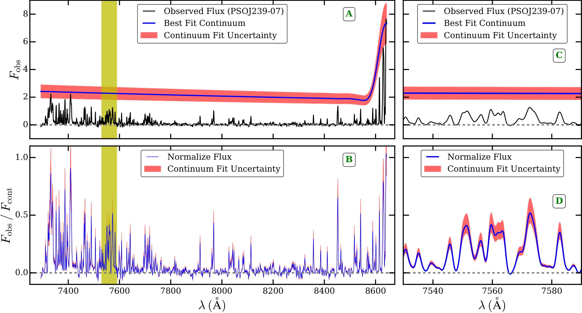
Due to the large opacities towards high redshift QSOs, the continuum placement is non-trivial. We explained the method of our continuum fitting in §2. The matching of the mean flux in observed and simulated spectra in a given redshift bin is affected by both the uncertainty in and the uncertainty in the continuum placement of the QSO. Unfortunately, there is significant uncertainty in both and continuum placement of QSOs at high redshift. Note however, that the scaling in flux is different for the two effects. While continuum errors affect the inferred flux level linearly, errors in the assumed in the simulated spectra affect the optical depth linearly, but the flux non-linearly due to the non-linear dependence of flux on optical depth (). Matching the observed mean flux by rescaling optical depth ( scaling) or rescaling flux (continuum uncertainty) have thus different effects on the transmission spikes. We illustrate the effect of flux scaling (continuum fitting uncertainty) on the spike statistics in Fig. 14 for the default simulation model. We calculate the three statistics by using a low continuum (), a default continuum () and a high continuum (). The normalization of the FPS and pCDDF is sensitive to the continuum placement. Somewhat surprisingly the continuum placement does, however, have very little effect on the spike width distribution. Note that the mean flux is different for the three models. We have looked in some detail into individual simulated spectra and found that for a lower placement of the continuum leading to a linear increase in observed flux levels the number of Voigt profile components increases. This appears to almost perfectly compensate for the expected increase in the width of individual components if the number of components stayed fixed for increased flux levels. Similarly, the effect of rescaling the optical depth (or ) is also small for the spike width distribution, but significant for pCDDF and FPS statistics (see Appendix B and Fig. 20 for details).
We illustrate the effect of continuum fitting uncertainty on the shape of transmission spikes in our observed spectra in Fig. 15. As already discussed the continuum placement uncertainty (shown by red shaded region in panel A and C), leads us to expect significant variation in the height of the spikes (panel D). However, the width distribution of the Voigt profile components of the fits to the transmission spikes is remarkably robust. To quantify the effect of the continuum on the observed transmission spikes, we show the three statistics in Fig. 16 by using again a low continuum (), a best fit continuum () and a high continuum (). Similar to Fig. 14, the normalization of the FPS and pCDDF in Fig. 16 is sensitive to the continuum placement. The continuum placement slightly changes the location of the peak in the spike width distribution and the distribution is somewhat broader for a low continuum. Note that the observed distributions are less well defined than those from our simulated spectra due to the small total number of spikes in our observed spectra compared to the simulated spectra1414 14 In Fig. 14, we calculated the statistics from simulated spectra.. We further emphasise again, that when comparing observed and simulated spectra we match the observed mean flux so there is a similar effect on the distributions of the simulated spectra. To demonstrate the expected effect of matching the observed mean flux, we have rescaled the optical depths inferred from the observed spectra (non-linear flux scaling) in the high and low continuum model such that the mean flux matches that with default continuum model. We call these continuum models “corrected” low or high continuum models (as shown by dotted lines in Fig. 16). The distributions for the corrected low and high continuum models are in very good agreement with that for the best fit continuum. This demonstrates that the effect of continuum fitting on spike statistics can indeed be minimized by rescaling the simulated optical depth to match the mean observed flux as discussed earlier for the simulated spectra.
A.2 Effect of S/N
In this section we illustrate the effect of finite S/N on the detectability of spikes. Since high- QSOs are usually faint and most of the observed pixels are close to , the noise in observed spectra is mostly determined by the sky background. Furthermore, the noise can vary along the wavelength axis. To minimize the effect of finite S/N on spike statistics, we degrade the simulated spectra with noise generated from the observed S/N per pixel array. The statistics computed from observed and simulated transmitted flux are consistent with each other. However, the ability of the Voigt fitting procedure crucially depends on the S/N of the spectra. To account for this, we compute a significance level (SL) for each Voigt component that accounts for the S/N, pixel separation and resolution of the instrument (Gaikwad et al. 2017b). We select the Voigt components with SL .
The finite S/N of the observed spectra also sets the completeness limit of the sample. However, one needs to account for the incompleteness of the sample for the lines with below the completeness limit. We account for the incompleteness of the sample by calculating the sensitivity curve as shown in Fig. 17. The plot shows the sensitivity curve for three redshift bins. The observed sample is 50 per cent complete for . We use the area under the curve to calculate the pCDDF and thus account for the effect of finite S/N.
Appendix B Sensitivity of spike statistics to astrophysical parameters
Fig. 18 to Fig. 22 shows the sensitivity of our chosen statistics to the normalization of the TDR (), the slope of TDR (), the H i photo-ionization rate () and Jeans smoothing, respectively. We vary , and in the post-processing step by using a power-law TDR and rescaling the optical depth under the assumption of photo-ionization equilibrium. This approach allows us to study the variation of spike statistics for a given parameter while keeping other parameters fixed.
Fig. 18 shows that all three transmission spike statistics are sensitive to . The spike width distribution (left panel in Fig. 18) is most sensitive to i.e., the spike width distribution is systematically shifted to larger values for hotter models. The shape of the pCDDF (middle panel in Fig. 18) is also sensitive to . This can be understood by examining Fig. 4, where we see that spikes in hotter models are usually more blended than cold models due to line of sight temperature and density smoothing effects. Due to such blending, viper fits fewer components with low and more components with high in hotter models. The FPS (right panel) is systematically lower at for K compared to K. This is expected as the increase in temperature smoothes the transmitted Ly flux, reducing the small scale power.
We illustrate the sensitivity of the three statistics to in Fig. 19. It is not possible to vary the slope of the TDR around the mean density without then varying the temperature at the density where the spikes are most sensitive. For example, the spikes in the optically thin simulations are most sensitive to (See Fig. 5). If we vary with the normalization of the TDR pivoted at , (i.e. the value), we obtain a large variation in temperature at . As a result it is hard to disentangle the effect of variation in from . To circumvent this problem, we pivot the TDR at the densities where spikes are most sensitive i.e., . Thus we use a power-law TDR of the form . The left and right panels in Fig. 19 show that the spike width distribution and FPS are less sensitive to the variation in . We see a slight variation in the shape of the pCDDF for a variation in , such that high systems are less frequent for than for . This is a direct consequence of the lower temperature at , since the spikes are more sensitive to than .
The effect of the photo-ionization rate is illustrated in Fig. 20. The heights and number of spikes (for a given S/N) are sensitive to . As a result, the normalization of the pCDDF is mostly sensitive to while the shape remains relatively unchanged. The normalization of the FPS depends on the mean transmitted flux, and since the mean transmitted flux varies with the normalization of the FPS is also different. However, the spike width distribution is relatively robust to large variations in , allowing one to minimize the degeneracy between and thermal parameters. Note the effect of continuum placement uncertainty is very similar to the variation in (see §A).
We show the recovery of and for fiducial hot and cold model in Fig. 21. We vary TDR using field from default model for a range of and . We use BPDF statistics to recover the and from hot and cold model. Fig. 21 demonstrate that we can recover and within for wide range of and .
We study the effect of pressure (or Jeans) smoothing in Fig. 22. We take the density and velocity fields from the default, hot and cold optically thin models and rescale the instantaneous temperatures and neutral hydrogen fractions to have the same values. Differences in the spike statistics due to pressure smoothing are therefore isolated from the effect of thermal broadening. In all three models reionization completes at , following the UVB synthesis model of Puchwein et al. 2019, with a total energy per proton mass of (default), (hot) and (cold) deposited over the redshift interval (Nasir et al. 2016, cf.). For comparison, Boera et al. 2019 have recently inferred over the redshift interval from new measurements of the Ly FPS at , which is consistent with our default simulation at . Interestingly, Fig. 22 shows that the spike width distribution is only modestly sensitive to the pressure smoothing, despite the different integrated thermal histories in the models. This is in part because, relative to the IGM at , gas has had slightly less time to dynamically respond to changes in the pressure following the completion of reionization at , and in part because the transmission spikes become rapidly more sensitive to the most highly underdense gas as redshift increases (where the dynamical time scales as ). We estimate that systematic uncertainties in the Jeans smoothing will therefore impact on the recovery of by at most (see Fig. 23). We add this uncertainty in quadrature to the final measurements we present for . We have furthermore verified if we take a more extreme model where the IGM is ionized rapidly around , (i.e. the fiducial model in the original Sherwood simulation suite), larger differences in the spike width distribution due to Jeans smoothing are present. We argue here, however, that such an early end to reionization is unlikely.
Appendix C Numerical effects
We assess the effect of simulation box size and mass resolution on convergence of the spike statistics in Fig. 24 and Fig. 25. We use simulations with varying box sizes and gas particle masses drawn from the optically thin Sherwood simulation suite (Bolton et al. 2017). All other parameters such as cosmology and the UVB evolution are same for the simulations. The spike statistics are well converged for our fiducial box size and mass resolution, which corresponds to the L40N2048 model.
Fig. 26 tests our method of constraining from the spike width distribution using a minimization process by evaluating the likelihood . The best fit model corresponds to a minimum , where our constraints on are contours of constant where we assume for 2 degrees of freedom (Avni 1976; Press et al. 1992). To a good approximation, we confirm the distribution in plane is Gaussian.

Appendix D Detailed comparison of statistics from observations with models
In this section, we first discuss quantitatively how well the spike width distribution, pCDDF and FPS statistics from optically thin and radiative transfer simulations fit the observed distributions. Table 4 shows the goodness of fit (reduced ) between model and observed statistics in the three redshift bins. The goodness of fit between observed spike width distribution for the default model is significantly better than that for the hot and cold models in all 3 redshift bins. The pCDDF and FPS statistics of the hot model are in somewhat better agreement with observations than the corresponding statistics of the default and cold models. Overall the default and hot models therefore show a better fit than the cold model. All three statistics for the aton model show a smaller than the patchy models, but the fits are generally reasonably good for both models. An exception to this is noticeable in the redshift bin, where the spike width distribution and FPS are marginally better fit by the patchy than by the aton model. When we compare the goodness of fit between optically thin and radiative transfer simulations we find the following. Formally the spike width distribution in the aton model is a better fit to observations than the default model (except at ). The of FPS and pCDDF statistics for the hot models are overall comparable to that from the aton model. However, FPS and pCDDF statistics are also sensitive to continuum placement uncertainty as shown in appendix A. Hence in this work, we have focused on the spike width distribution for constraining and . As discussed in detail in the main text we consider the radiative transfer models aton and patchy as more physical than the default and hot model because they account for spatial fluctuations of the UVB and TDR. As discussed in the introduction such fluctuations are important for producing the observed scatter and long absorption troughs at these redshifts.
| Simulation | pCDDF | FPS | pCDDF | FPS | pCDDF | FPS | |||
|---|---|---|---|---|---|---|---|---|---|
| default | 2.27 | 4.01 | 1.00 | 1.10 | 0.68 | 0.84 | 0.88 | 0.49 | 0.52 |
| cold | 14.69 | 15.24 | 6.69 | 10.08 | 2.82 | 0.79 | 11.40 | 1.47 | 0.89 |
| hot | 5.10 | 1.60 | 0.62 | 5.26 | 0.57 | 1.34 | 1.12 | 0.31 | 0.36 |
| aton | 1.91 | 2.06 | 0.63 | 1.51 | 0.55 | 1.66 | 0.49 | 0.35 | 0.24 |
| patchy | 3.60 | 3.11 | 1.52 | 1.17 | 0.74 | 1.59 | 1.44 | 0.92 | 0.39 |