Efficient Algorithms towards Network InterventionConference: Proceedings of The Web Conference 2020; April 20–24, 2020; Taipei, TaiwanProceedings of The Web Conference 2020 (WWW ’20), April 20–24, 2020, Taipei, Taiwan
Abstract.
Research suggests that social relationships have substantial impacts on individuals’ health outcomes. Network intervention, through careful planning, can assist a network of users to build healthy relationships. However, most previous work is not designed to assist such planning by carefully examining and improving multiple network characteristics. In this paper, we propose and evaluate algorithms that facilitate network intervention planning through simultaneous optimization of network degree, closeness, betweenness, and local clustering coefficient, under scenarios involving Network Intervention with Limited Degradation - for Single target (NILD-S) and Network Intervention with Limited Degradation - for Multiple targets (NILD-M). We prove that NILD-S and NILD-M are NP-hard and cannot be approximated within any ratio in polynomial time unless P=NP. We propose the Candidate Re-selection with Preserved Dependency (CRPD) algorithm for NILD-S, and the Objective-aware Intervention edge Selection and Adjustment (OISA) algorithm for NILD-M. Various pruning strategies are designed to boost the efficiency of the proposed algorithms. Extensive experiments on various real social networks collected from public schools and Web and an empirical study are conducted to show that CRPD and OISA outperform the baselines in both efficiency and effectiveness.
Keywords:
Network intervention, optimization algorithms, social networks1. Introduction
Previous studies have shown the importance and strengths of social relationships in influencing individual behaviors. Strong social relationships have been shown to facilitate the dissemination of information, encourage innovations, and promote positive behavior (Valente 2012). Also, social relationships surrounding individuals have substantial impacts on individuals’ mental and physical health (Dhand et al. 2016; House et al. 1988). For example, studies in Science and American Sociological Review indicate that socially isolated individuals are more inclined to have mental health problems and physical diseases, ranging from psychiatric disorders to tuberculosis, suicide, and accidents (House et al. 1988; Durkheim 1951).
To alleviate the problems that arise with social isolation, two classes of intervention strategies may be adopted, including: 1) personal intervention, which guides individuals to understand their situations, attitudes, and capacities through counseling (Cohen et al. 2000); and 2) network intervention, which emphasizes the need to strengthen individuals’ social networks to accelerate behavior changes that can lead to desirable outcomes at the individual, community, or organizational level (House et al. 1988; Dhand et al. 2016). As an example, network intervention that helps establish new social links is crucial for individuals with autism spectrum disorders (Chang and Locke 2016). Those new links may be effectively introduced by curative groupings and network meetings — events which encourage them to socialize more frequently (Erickson 1984; De La Haye et al. 2011).
In order for network intervention to improve individual health outcomes, it is crucial to add social links in ways that promote network characteristics found to be related to positive outcomes. Thus, an important question to ask is: given an individual, what properties define the strength of the individual’s network? Previous studies point out several possibilities: 1) Degree indicates the number of established friendships. An individual with a large degree is more popular and has more opportunities to establish self-identity and social skills (Ueno 2005). Thus, a large-degree individual is less inclined to be socially-isolated and have mental health problems (Durkheim 1951). 2) Closeness indicates the inverse of the average social distance from an individual to all others in the network. An individual with great closeness is typically located in the center of the network and tend to perceive a lower level of stress (Howell et al. 2014). 3) Betweenness indicates the tendency of an individual to fall on the shortest path between pairs of other individuals. An individual with large betweenness tends to occupy brokerage positions in the network and have more knowledge of events happening in the network. Thus, an individual with large betweenness may also perceive social relationships more accurately (Lee et al. 2017). 4) Finally, Local clustering coefficient (LCC) indicates the diversity of relationships within an individual’s ego network (Dhand et al. 2016). Specifically, an individual with a small LCC tends to have diverse relationships since her friends are less likely to be acquainted with each other (Dhand et al. 2016). The perspective that individuals with small LCCs are less likely to have mental health problems has been postulated in the functional specificity theory, which advocates the need for having different support groups for distinct functions e.g., by obtaining attachment from families or friends, social integration from social activity groups, and guidance from colleagues (Weiss 1974). In other words, individuals with large LCCs tend not to build a diverse social network by putting all their relationship eggs in a few baskets, and tend to have depressive symptoms and neurological illnesses (Dhand et al. 2016). This relationship has been validated in studies with participants across various cultures and ages. In a study involving 173 retired US elders, higher LCC is found to be associated with lower life satisfaction, self-esteem, happiness, and higher depression (Yuan et al. 2017). In another study involving 2844 high school students, higher LCC again is associated with lower self-esteem (TYP 2018).
In practice, specialists and practitioners may not have the time or resources to provide frequent and ongoing relationship recommendations to every individual. Also, the recommendations made by persons are susceptible to their subjective biases. As such, supplemental, objective information from automated network planning algorithms that can simultaneously optimize multiple network characteristics are helpful and valuable. This paper aims to develop novel algorithms that recommend suitable intervention links based on multiple potentially health-enhancing network characteristics. However, adding social links is not always straightforward for network characteristics. Of the characteristics noted earlier, the degree for each individual can be improved by adding more edges, in which case the closeness and betweenness of the network are also enhanced. However, improving the LCC is more challenging as the LCCs of individuals and nearby friends may not always improve, and they can even deteriorate, when more edges are added.


Selecting good intervention links based on the LCC is further deterred by other challenges. A new link established for a targeted individual may increase the LCCs of her friends, when those new friends are acquainted with each other. Figure 1 presents an example showing the side-effects of adding improper new links on the LCC. Figure 1(a) shows a social network in which the nodes are annotated by their initial LCCs, and Figure 1(b) presents the network after adding an edge from B to G. The LCC of B is effectively reduced to 0.5, but the LCC of C unfortunately grows to 0.66. The example shows that heuristic or uninformed selection of intervention links by specialists and practitioners may lead to undesirable changes in the LCC; even worse, the undesirable changes may happen to many nearby individuals when the network size is large. Moreover, even though a simple way to decrease LCC is to remove some existing social links, this approach is not considered because removal of existing social links undermines established social support (Thoits 1983).
In this paper, we propose and test several algorithms that can simultaneously optimize network LCC, closeness, betweenness, and degree. We first formulate a new problem, namely, Network Intervention with Limited Degradation - for Single target (NILD-S). Given a budget of , a threshold , and a target , NILD-S finds the set of intervention edges to minimize the LCC of , such that the side effect, in terms of increment in anyone’s LCC, cannot exceed . NILD-S also ensures that the degree, betweenness and closeness of exceed given thresholds. We propose Candidate Re-selection with Preserved Dependency (CRPD) algorithm, which first obtains an initial solution by extracting the individuals with the smallest degrees, and improves the initial solution by re-examining the candidates filtered out by nodes involved in the solution. Note that CRPD selects edges according to multiple characteristics. We prove that NILD-S is NP-hard and cannot be approximated within any ratio in polynomial time unless P=NP. Nevertheless, we prove that CRPD can find the optimal solution for threshold graphs, which are very similar to many well-known online social networks regarding many measurements like degree distribution, diameter and clustering coefficient (Masuda et al. 2004; Vernitski and Pyatkin 2012; Saha et al. 2014).
Finally, we seek to extend the NILD-S to simultaneously improve the LCCs of multiple individuals while ensuring other network characteristics, including betweenness, closeness, and degree. To do so, we formulate the Network Intervention with Limited Degradation - for Multiple targets (NILD-M) problem to jointly minimize the LCCs of multiple targets. Given the aforementioned , , and the set of targets , NILD-M finds the set of intervention edges such that the maximal LCC of individuals in is minimized, while the LCC increment of any person does not exceed . NILD-M also ensures that the degree, betweenness, and closeness of all targetes exceed their minimum thresholds. We prove that NILD-M is NP-hard and cannot be approximated within any ratio in polynomial time unless P=NP. To solve NILD-M, we design Objective-aware Intervention edge Selection and Adjustment (OISA), which 1) carefully examines both the LCC of each terminal and the network structure to ensure the constraint of , 2) explores the idea of optionality to improve the solution quality, and 3) derives the lower bound on the number of required edges and the LCC upper bounds to effectively reduce computational time. Also, we evaluate OISA via an empirical study on four psychological outcomes, anxiety, perceived stress, positive and negative emotions, and psychological well-being.
The contributions are summarized as follows.
- •
Previous research has suggested the use of network intervention in improving health outcomes. With the potential to increase the support network by new acquaintances, however, there is no effective planning tool for practitioners to select suitable intervention edges. We formulate NILD-S and NILD-M to address this critical need for identifying suitable intervention links for a single target and a group of targets, while considering multiple network characteristics.
- •
We prove that NILD-S is NP-hard and cannot be approximated within any ratio in polynomial time unless P=NP. We propose CRPD and prove that CRPD obtains the optimal solution for threshold graphs.
- •
We prove that NILD-M is NP-hard and cannot be approximated within any ratio in polynomial time unless P=NP and design OISA for NILD-M.
- •
Experiments on real datasets show that the proposed CRPD and OISA efficiently find near-optimal solutions for NILD-S and NILD-M and outperform the baselines. Also, an empirical study assessed by clinical psychologists and professors in the field manifests that the network intervention alleviates self-reported health outcomes of participants, and the effects are statistically significant over another control group.
The rest of this paper is organized as follows. Section 2 reviews related work. Section 3 formulates NILD-S, analyzes its theoretical hardness, and proposes CRPD. Section 4 formulates NILD-M and analyzes its theoretical hardness. Section 5 proposes OISA. Section 6 reports the experiments. Finally, Section 7 concludes the paper.
2. Related Work
The theory of network intervention has been studied in the fields of psychology, behavioral health, and education for lowering negative emotions by enhancing social integration, support, engagement, and attachment (Berkman et al. 2000). It has also been adopted for family therapy and bullying avoidance (Erickson 1984). In education, network intervention has been implemented to facilitate knowledge dissemination among students, thereby improving student learning (Van Den Oord and Van Rossem 2002). Under current practice, new intervention links are typically selected heuristically by practitioners (King et al. 2006; Sherman et al. 2009). However, it is very challenging to consider multiple persons simultaneously without deteriorating the status of surrounding individuals. Thus, it would be worthwhile to develop algorithms for this important need.
In the field of social network analysis, researchers have paid considerable attention to efficiently finding the number of triangles (Lim and Kang 2015; McGregor et al. 2016) and selecting a group of individuals with the maximum or minimum number of triangles (Shen et al. 2017). Notice that the above-mentioned research mostly focuses on measuring structural properties of nodes in static or dynamic networks, with no intention to tailor and change the network graph. Recently, a new line of research in network science has emerged with the objective of revising a network graph according to specific network characteristics. These include maximizing the closeness centrality, betweenness centrality and influence score, minimizing the diameter, and enhancing the network robustness (Papagelis 2015; Crescenzi et al. 2016; Wilder et al. 2018). However, these algorithms do not include LCC as a target network characteristic for intervention purposes. Importantly, none of these algorithms was designed to optimize multiple network characteristics simultaneously.
Recently, owing to the success of online social networks, reported cases of social network mental disorders have increased, motivating new collaborations between data scientists and mental health practitioners. New machine learning frameworks have been shown to be helpful in identifying patients tending to be vulnerable, and even have clinical levels of negative emotions and unhealthy living (Shuai et al. 2016; Saha et al. 2016; Shuai et al. 2019; Shuai et al. 2017). However, those are not designed for network intervention, which actually changes the network graph. Finally, link prediction (Scellato et al. 2014; Barbieri et al. 2014; Wang et al. 2018; Brochier et al. 2019; Chen et al. 2018; Zhang and Chen 2018; Fu et al. 2018) has been widely studied. Existing algorithms usually recommend individuals sharing many common friends and similar interests to become friends. However, they are not designed for network intervention, which does not necessarily prefer people socially close or with similar backgrounds.
| Term | Meaning | Term | Meaning |
|---|---|---|---|
| original network | selected intervention edges | ||
| , | targeted individual(s) | network after intervention | |
| ’s neighbors in | node to be connected with | ||
| ’s betweenness in | maximum degree in | ||
| ’s closeness in | nodes removed by CRPD baseline | ||
| ’s degree in | a removed node in | ||
| ’s LCC in | weights of betweenness in MISS | ||
| lower bound of betweenness | weights of closeness in MISS | ||
| lower bound of closeness | weights of degree in MISS | ||
| lower bound of degree | weight func. in threshold graph | ||
| LCC degradation constraint | lower bound on the num. of | ||
| # of intervention edges | needed edges in EORE | ||
| # of edges among ’s neighbors | targeted LCC to be tried in EORE |
3. Intervention for A Single Target
In this section, we first reduce the Local Clustering Coefficient (LCC) of a targeted individual (denoted as ) by selecting a set of people from the social network to become friends with . Given a social network (or for short), where each node denotes an individual, and each edge represents the social link between individuals and , the ego network of an individual is the subgraph induced by and its neighbors . The LCC of a node in , , is defined as the number of edges between the nodes in divided by the maximum number of possible edges among the nodes in ,
| (1) |
where and is the number of combinations to choose two items from ones. Adding social links may increase LCC of other nodes not incident to any new edge.
However, the increment of LCC for healthy people also needs to be carefully controlled.11 1 According to the study on 2844 junior high school students over three years (TYP 2018), the decrement of depression rates is significantly correlated with the reduction of LCCs with Pearson Correlation Coefficient as 0.3. In addition to LCC, it is also important to ensure that the degree, betweenness, and closeness are sufficiently large. Therefore, we formulate the Network Intervention with Limited Degradation - for Single target (NILD-S) problem as follows.
Definition 0.
Given a social network (or for short), the target , the number of intervention edges to be added, the LCC degradation threshold , the lower bounds on betweenness, closeness and degree , , and , NILD-S minimizes the LCC of by adding a set of edges incident to , such that in the new network , 1) for any , 2) , 3) , and 4) , where , and are the betweenness, closeness, and degree of in .
NILD-S is computationally expensive. We prove that it is NP-hard and inapproximable within any ratio, i.e., there is no approximation algorithm with a finite ratio for NILD-S unless P=NP. However, later we show that NILD-S is tractable for threshold graphs, which share similar graph properties with many well-known online social networks, e.g., Live-Journal, Flickr, and Youtube (Masuda et al. 2004; Vernitski and Pyatkin 2012; Saha et al. 2014).
Theorem 2.
NILD-S is NP-hard and cannot be approximated within any ratio in polynomial time unless P=NP.
Proof.
We prove the NP-hardness by the reduction from the Maximum Independent Set (MIS) problem under triangle-free graphs (i.e., a graph without any three nodes forming a triangle) (Lozin and Milanič 2008). Given a triangle-free graph , MIS is to find the largest subset of nodes , such that every node in is not adjacent to any other nodes in . For each instance of MIS, we construct an instance of NILD-S as follows. For each node and edge , we create the corresponding node and edge , respectively. Also, we add a node as the targeted node and set , , , and as 0. In the following, we prove that has an independent set with size in MIS if and only if the LCC of in remains as 0 after adding for every . We first prove the sufficient condition. If has an independent set of size , then there is no edge between any two nodes in . Thus, if we add an edge for each node in , the LCC of is still 0. We then prove the necessary condition. If there is a set of nodes such that ’s LCC remains as 0 after adding to , then there exists no edge among ’s neighbors, i.e., . Therefore, with the corresponding nodes in is an independent set.
Next, we prove that NILD-S cannot be approximated within any ratio in polynomial time unless P=NP by contradiction. Assuming that there exists a polynomial-time algorithm with solution to approximate NILD-S with a finite ratio for a triangle-free , i.e., the LCC of the optimal solution is at least . If , there is an independent set with size . If , the LCC of the optimal solution is at least , and there is no -node independent set. Thus, the approximation algorithm for NILD-S can solve MIS in polynomial time by examining , contradicting that MIS is NP-hard (Lozin and Milanič 2008). ∎
3.1. The CRPD Algorithm
For NILD-S, a simple approach is to iteratively choose a node , add into , and eliminate (i.e., does not regard it as a candidate in the future) every neighbor of if adding both and into would increase the LCC of any node for more than (called the LCC degradation constraint). However, the above approach does not carefully examine the structure among the neighbors of . The selection of is crucial, because it may become difficult to choose its neighbors for connection to later due to the LCC degradation constraint. Therefore, a simple baseline is to extract the with the smallest degree and add to , because such tends to result in the least number of neighbors removed from the pool of candidates for connecting to . It removes those neighbors of if adding increases LCC of any individual by more than . However, Example 2 indicates that a good candidate may be improperly removed due to a small LCC.


Example 0.
Figure 3 shows an example of NILD-S with 16 nodes, where , , , , , and . Note that all edges in Figure 3 are edges in regardless of their colors. The baseline first selects (i.e., adding to ) since it has the smallest degree among all nodes not connected to . Then, for the neighbor of , adding to does not increase LCC of any node to more than . Thus, is still a valid candidate.22 2 Adding to only changes the LCCs of and , where and . However, after choosing , the baseline excludes and from candidates as their respective LCCs will be increased by 0.06. Afterward, the baseline selects and to reduce the LCC of from 1 to 0.2. Nevertheless, a better approach is to select , and , as the LCC of can effectively diminish to 0.1.
Motivated by Example 2, we propose the Candidate Re-selection with Preserved Dependency (CRPD) algorithm for NILD-S. CRPD includes two components: 1) Removed Node Re-selection Strategy, and 2) Multi-measurement Integration Selection Strategy, as follows. A pseudocode of CRPD is shown in Algorithm 1.
Removed Node Re-selection (RNR) Strategy. To avoid missing good candidates when processing each node in the above baseline, CRPD first extracts during the process, where each in is a neighbor of removed by the baseline due to the LCC degradation constraint, i.e., including both and in increases any node’s LCC for more than . CRPD improves the above baseline by conducting a deeper exploration that tries to replace by , where is the node with the minimum degree in , if selecting instead removes fewer neighbors and obtains a better solution later. In Example 2, adding to removes its neighbors and because including or to increases the LCCs of or by more than , respectively. In contrast, adding (instead of ) to only removes and obtains a better solution , compared with the solution of the baseline. With the above deeper inspection, later we prove that CRPD can find the optimal solution of NILD-S in threshold graphs.
Multi-measurement Integration Selection Strategy (MISS). To address , the degree of can be examined according to when more edges are included. However, when the betweenness and closeness of are smaller than and , respectively, CRPD selects as follows to improve the betweenness and closeness of , when multiple nodes available to be chosen as .
| (2) |
where and denote the betweenness and closeness of , and and are the weights of betweenness and closeness in selecting . (or ) is derived by computing the difference of ’s betweenness and (or ’s closeness and ) when ’s betweenness (or closeness) is smaller than (or ). Otherwise, (or ) is set as 0.
3.2. Solution Quality in Threshold Graph
We prove that CRPD obtains the optimal solution for threshold graphs, which are similar to many well-known online social networks in terms of important properties like the scale-free degree distribution, short diameter, and clustering coefficient (Masuda et al. 2004; Vernitski and Pyatkin 2012; Saha et al. 2014).
Definition 0.
A graph is a threshold graph if there exists a weight function and a threshold , such that for any two nodes , if and only if .
Theorem 5.
The CRPD algorithm can find an optimal solution of NILD-S when is a threshold graph, and the running time of CRPD is , where is the maximum degree in .
With the property of threshold graphs, we prove that CRPD always finds a feasible solution, and the obtained feasible solution is one of the optimal ones in Appendix A.1.
4. Intervention for Multiple Targets
We formulate the Network Intervention with Limited Degradation - for Multiple targets (NILD-M) problem and show the NP-hardness.
Definition 0.
Given a social network (or for short), the number of intervention edges to be added, the LCC degradation threshold , the lower bounds on betweenness, closeness and degree , , and , and a set of targeted individuals , the NILD-M problem minimizes the maximal LCC among all nodes in , i.e., , by selecting a set of intervention edges , such that in the new network , 1) for any , 2) for any , 3) for any , and 4) for any , where , and are the betweenness, closeness, and degree of in .
Corollary 0.
NILD-M is NP-hard and cannot be approximated within any ratio in polynomial time unless P=NP.
5. The OISA Algorithm
A naïve approach for NILD-M is to exhaustively search every -edge set spanning the nodes in . However, the approach is not scalable as shown in Section 6. In the following, we first present two baseline heuristics, Budget Utility Maximization (BUM) and Surrounding Impact Minimization (SIM) for NILD-M.
Budget Utility Maximization (BUM). To intervene the maximal number of individuals within , BUM repeatedly selects the node having the largest LCC without contradicting any constraints and connects to the node with the largest LCC in until edges are selected.
Surrounding Impact Minimization (SIM). Without considering the proximity between and , adding sometimes increases the LCCs of their common neighbors. To avoid the above situation, SIM chooses the with the maximum number of hops from in because adding is less inclined to change the LCCs of other neighbor nodes.
In summary, BUM carefully evaluates the LCC of but ignores the structural properties, whereas SIM focuses on the distance between and but overlooks the LCC. Be noted that BUM and SIM are also equipped with MISS to ensure they obtain feasible solutions. Example 1 indicates that their solutions are far from the optimal solution.
Example 0.
Figure 3 presents an example with and . includes 14 nodes and 23 black solid edges, where each node is labeled aside by its in dark. The targeted includes 8 grey nodes with the largest LCC in , i.e.,
. , , are set as 0.02, 0.44, and 3, respectively.
The weights , , and of MISS are set as 0.33, 0.33, and 0.34.
For this instance, the maximal LCCs obtained by BUM and SIM are both 1. In contrast, the maximal LCC in the optimal solution is 0.66 acquired by adding the dotted blue edges into . For each node whose is not equal to , its are labeled aside in red. The optimal solution effectively lowers the maximal LCC by 34% from BUM and SIM without increasing any node’s LCC.
Motivated by the strengths and pitfalls of BUM and SIM, we propose Objective-aware Intervention Edge Selection and Adjustment (OISA) to jointly consider the LCCs and the network structure with three ideas: 1) Expected Objective Reaching Exploration (EORE), and 2) Poor Optionality Node First (PONF), and 3) Acceleration of LCC Calculation (ALC). EORE finds the minimum number of intervention edges required to achieve any targeted LCC for each candidate solution and sees if it can meet the budget constraint . Given a targeted LCC, PONF carefully adds intervention edges to avoid seriously increasing LCCs for some individuals. A pseudocode of OISA is shown in Algorithm 2.
5.1. Expected Objective Reaching Exploration
EORE carefully examines the correlation between the LCC reduction and the number of intervention edges. Lemma 2 first derives the minimum number of required intervention edges for to achieve any targeted LCC. To meet the degree constraint , the minimum number of edges for each node is at least .
Lemma 0.
Given a node of degree , to reduce
to any targeted LCC , the minimum number of intervention edges is the smallest number satisfying:
| (3) |
Also, the minimum number of edges for is
(proof in Appendix A.2).
Equipped with Lemma 2, a simple approach is to examine every possible LCC, i.e., , where is the maximum degree among all nodes in . However, since adding edges can make intervention for at most nodes, it is not necessary to scan all possible LCCs, and EORE thereby only examines a small number of targeted LCCs , where with , until exceeds the maximal LCC before intervention, and is the maximum degree among all top- nodes with the largest LCCs in . OISA skips an if according to the above lemma.
For any targeted LCC , every node requires at least intervention edges to achieve the targeted LCC and the degree constraint. Thus, OISA stops the edge selection process if there exists a node not able to achieve the above goals when , where is the number of intervention edges incident with in .
Example 0.
For the example in Figure 3, the node with the maximum degree among the top- nodes with the largest LCCs is , where its degree is 4. The targeted LCCs to be examined (i.e., ) are 0.17, 0.33, 0.5, 0.67, 0.83, 1. For the targeted LCC , is since for , and for , , , , , , and . However, for the targeted LCC , is since for , and for , , , , , , and . Thus, it is impossible for the maximal LCC to reach 0.17.
5.2. Poor Optionality Node First
Recall that BUM ignores the proximity between the two terminal nodes of an intervention edge, and SIM does not examine the LCCs of both terminals and their nearby nodes. Most importantly, both strategies do not ensure the LCC degradation constraint. To address this critical issue, for each targeted LCC, we first propose the notion of optionality to identify qualified candidate intervention edges that do not increase the LCC of any individual to more than .
Definition 0.
Optionality. For a target , the optionality of denotes the number of nodes in the option set such that for every , either 1) the hop number from to is no smaller than 3, or 2) is two-hop away from and adding an edge does not increase the LCC of any common neighbor by more than .
For the first case, adding an intervention edge does not increase the LCC of any node. For the second case, the LCC degradation constraint can be ensured as long as the LCCs of common neighbors are sufficiently small. Equipped with the optionality, each iteration of PONF first extracts the node with the largest LCC in . If there are multiple candidates for with the same LCC, (e.g., and in Figure 3), PONF selects the one with the smallest optionality as so that others with larger optionalities can be employed later. In contrast, if was not selected by now, its optionality tends to decrease later when the network becomes denser and may reach 0, so that the LCC of can no longer be reduced without increasing the LCCs of others, boosting the risk to violate the LCC degradation constraint. The node of the intervention edge is the one with the largest LCC in the option set to reduce the LCCs of both and . PONF also exploits MISS in Section 3.1 to choose according to the differences between ’s betweenness and , and between ’s closeness and .
Example 0.
For the example in Figure 3 with the targeted LCC as 0.33, one intervention edge is selected for , , , , and . In the first iteration, the optionalities of nodes , , , , and are 7, 5, 5, 5, 6, and 7, respectively. The option set of is . Thus, PONF chooses as and as . Note that is the node with the largest difference to reach , , and according to Equation 2. In the second iteration, the optionality of , , , and are 7, 5, 6, 7, respectively. Thus, PONF selects as and as . It repeats the above process and chooses and afterward. Figure 3 shows the returned solution with the maximal LCC as 0.33. It is also the optimal solution in this example.
5.3. Acceleration of LCC Calculation
When an edge is added, only the LCCs of and and their common neighbors are likely to change. However, the LCC update cost of is not negligible when the number of neighbors is huge, since it needs to examine whether there is an edge from to each of ’s neighbors. The adjacency list of every ’s neighbor is required to be inspected even when the LCC of remains the same. To improve the efficiency, ALC avoids examination of every node by deriving its LCC upper bound .
Definition 0.
The LCC upper bound of after adding edges is
| (4) |
where is the degree of in . is the number of edges between ’s neighbors before intervention, .
Theorem 7.
For an intervention edge set of size ,
holds.
Proof.
Let and denote the numbers of intervention edges connecting to and any two neighbors of , respectively. After intervention, , and , where is the number of edges between the new neighbors via the new edges and the original neighbors of in , and . Thus, . Let .
Then, we obtain
.
∎
According to the above theorem, ALC first derives and as a pre-processing step of OISA before intervention. Accordingly, PONF does not update the LCC of a node if the intervention edge neither connects to nor spans ’s two neighbors, and is not going to be and in the next iteration since is smaller than the current maximal LCC potential to be and in the next iteration. Therefore, Theorem 7 enables OISA to effectively skip the LCC updates of most nodes.
Theorem 8.
The time complexity of OISA is , where is the number of targeted LCCs, and is the number of nodes with the largest LCC (proof in Appendix A.3).
6. Experimental Results
We evaluate the effectiveness and efficiency of CRPD and OISA by experimentation in Sections 6.1 and 6.2, respectively. Also, to show the feasibility of using OISA in real-world setting, we present an empirical study in Section 6.3.33 3 The IRB number is 10710HE072. The study has been inspected by 11 clinical psychologists and professors in the field.44 4 They are from California School of Professional Psychology, Taipei City Government Community Mental Health Center, National Taipei University of Nursing and Health Science, National Taiwan University etc.
| dataset | ave. LCC | dataset | ave. LCC | ||||
|---|---|---|---|---|---|---|---|
| CPEP (Gest et al. 2014) | 226 | 583 | 0.71 | Youtube (SNAP 2018) | 1.1M | 3.0M | 0.08 |
| Facebook (Viswanath et al. 2009) | 60.3K | 1.5M | 0.22 | Amazon (SNAP 2018) | 33.5K | 92.6K | 0.40 |
| Flickr (Mislove et al. 2007) | 1.8M | 22.6M | 0.25 | Cond-Mat (SNAP 2018) | 23.1K | 93.5K | 0.63 |
For simulation, since there is no prior work on lowering LCCs while ensuring their betweenness, closeness and degree, we compare the proposed CRPD and OISA with five baselines: 1) Budget Utility Maximization (BUM): BUM iteratively adds an edge between a targeted node and the node with the largest LCC, while not violating the constraints; 2) Surrounding Impact Minimization (SIM): SIM iteratively adds an edge from a targeted node to the node with the maximal number of hops from it, while not violating the constraints; 3) Enumeration (ENUM): ENUM exhaustively finds the optimal solution. 4) Edge Addition for Improving Network Centrality (EA) (Papagelis 2015): EA iteratively adds an edge with the largest increment on closeness centrality, and 5) Target-oriented Edge Addition for Improving Network Centrality (TEA) (Crescenzi et al. 2016): TEA iteratively adds an edge with the largest increment on closeness centrality for the targeted nodes. 6) Greedy algorithm for Dyad scenario (GD) (Wilder et al. 2018): GD iteratively adds an edge with the largest increment on influence score, where the influence score is calculated in a similar way to PageRank. All algorithms are implemented on an HP DL580 G9 server with four Intel Xeon E7-8870v4 2.10 GHz CPUs and 1.2 TB RAM. Six real datasets are evaluated in the experiments. The first one, CPEP (Gest et al. 2014), contains the complete social network of the students in 10 classrooms of several public elementary schools in the US. The other five large real social network datasets, collected from the Web, are Facebook, Flickr, Youtube, Amazon, and Cond-Mat. Some statistics of datasets used in our experiments are summarized in Table 2. The default , and are set to , , and , respectively.
6.1. Evaluation of CRPD for NILD-S


In the following, we first compare CRPD with baselines by varying . For Facebook and Flickr, ENUM does not return the solutions in two days even when , and thus it is not shown. Figures 4(a)-(e) compare the results of various on CPEP and Flickr under default , and . For CPEP, is set to 6%, 12%, 18%, 25%, and 31% of the number of nodes (i.e., 1, 2, 3, 4, and 5 intervention edges). For Flickr, is set to 0.02%, 0.04%, 0.06%, 0.8%, and 0.1% of nodes (i.e., 400, 800, 1200, 1600, and 2000 intervention edges). The is randomly chosen from the nodes with LCC larger than 0.8, and we report the average of 50 trials. Figures 4(a) and 4(b) show that with increasing, ’s LCC decreases as more edges are connected with to reduce its LCC. Also, CRPD outperforms other baselines as it carefully examines the candidates’ structure to avoid increasing the number of edges among ’s neighbors. Figure 4(c) shows the running time of OISA is comparable with simple baselines BUM and SIM while achieving better LCC on Flickr.
Figures 4(d) and 4(e) show the betweenness and closeness of after adding the intervention edges to Flickr. EA and TEA obtain the largest betweenness and closeness, but their maximal LCCs are not effectively reduced. SIM also achieves large betweenness and closeness since it selects the node farthest from as and creates a shortcut between them, but the maximal LCC of SIM does not significantly decrease. GD achieves smaller betweenness and closeness than SIM since it generally selects a node with a large PageRank score, but its improvement on ’s betweenness and closeness is smaller than SIM. BUM induces the smallest betweenness and closeness of since it selects with the largest LCCs, and those chosen are inclined to be near each other. In contrast, CRPD achieves comparable performance with EA and TEA, showing that CRPD can effectively improve not only LCC but also other network characteristics.
Next, we conduct a series of sensitivity tests on , , and , and show the component effectiveness. The results on CPEP and Facebook are similar to Flickr and thus not shown here.
Varying . Figure 4(f) compares LCC of with different on Flickr, under default and . As shown, the LCC of decreases because a large allows more nodes to be candidates and thereby tends to generate a better solution. Figure 4(g) shows that the running time of CRPD and baselines on Flickr increases as grows because more candidates are considered.
Varying and . Figure 4(h) compares the LCC of with different on Flickr, where (800 intervention edges). The trend of is similar to that of and thus not shown here. LCC of slightly grows with increasing and , because large and require CRPD and baselines to allocate more edges for the betweenness and closeness, instead of focusing on reducing LCC. Moreover, LCC of obtained by TEA, EA, and CRPD increases slower than one obtained by BUM, SIM and GD, since the edges selected by TEA and EA maximize the closeness centrality while fulfilling the constraints of and , whereas the edges from CRPD effectively increase the betweenness and closeness of .
Component Effectiveness. Figure 4(i) compares LCC of obtained by CRPD with and without RNR, and Figure 4(j) compares the closeness of CRPD with and without MISS on Flickr. The trend of betweenness is similar to closeness and thereby not shown here. As shown, while CRPD with and without MISS shares similar LCCs, CRPD with MISS achieves a greater closeness because choosing with larger closeness/betweenness tends to increase ’s betweenness and closeness. The results of CRPD on CPEP and Facebook share a similar trend and thus are not shown here.
6.2. Evaluation of OISA for NILD-M
In the following, we evaluate the proposed OISA by randomly choosing 20% of nodes in as from the nodes with the top-40% maximum LCCs. The results are the average of 50 trials.


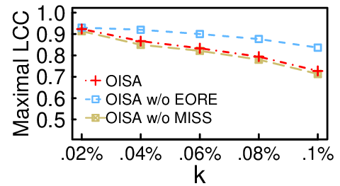
Figures 5(a)-(c) first compare the effectiveness of all examined approaches on CPEP by varying the number of intervention edges (relative to the edge number in ). Figure 5(a) indicates that as grows, the maximum LCC generally decreases. OISA and ENUM significantly outperform BUM, SIM, EA, TEA, and GD because EA, TEA and GD are designed to maximize the closeness centrality and influence score, instead of reducing the maximum LCC.Also, BUM only examines the LCCs of the nodes, while SIM ignores LCCs and gives the priority to the intervention edges with the maximum numbers of hops. Figure 5(b) presents the running time of all approaches in the log-scale. OISA and most baselines select within 1 second. In contrast, the running time of ENUM grows exponentially.
To understand the changes of LCCs in different nodes, we take a closer look at the nodes whose LCC potentially changes, i.e., the terminal nodes of the selected edges and their neighbors. Figure 5(c) presents the average LCC change of the nodes in each LCC range after intervention where . As shown in Figure 5(c), even though BUM outperforms SIM, the average LCC reduction in the range [0.9, 1] is smaller than SIM since BUM may connect nearby nodes and increase the LCCs of the common neighbors. It also explains why the maximum LCC achieved by BUM drops slower than SIM, ENUM, and OISA while increases, i.e., BUM creates lots of targeted nodes with LCCs around 0.6 and 0.7, and BUM needs to make intervention for all of them again to reduce the maximum LCC to become lower than 0.6. In contrast, the behavior of OISA is similar to ENUM in most ranges, and it successfully achieves comparable performance.
Next, Figures 5(d)-(i) compare all approaches except ENUM on Flickr, since ENUM does not return any solution in two days even for . The result on Facebook is similar and thereby is not shown here. As there are nearly 9000 nodes with LCCs as 1 on Flickr, the minimal is 4500 edges, because adding one edge can make intervention for at most two nodes with LCC as 1. Thus, is set to 0.02%, 0.04%, 0.06%, 0.08%, and 0.1% of the number of edges (i.e., 4500, 9000, 13500, 18000, and 22500 edges). Figure 5(d) indicates that OISA significantly outperforms all other baselines under all settings of . BUM is superior to SIM when is small because the farthest node selected by SIM usually results in a small LCC and fewer neighbors, i.e., reducing the LCC of does not help reduce the maximum LCC. Thus, when the number of intervention edges to be added is small, e.g., smaller than the number of targeted nodes in , it is impossible for SIM to reduce the maximum LCC. In contrast, selected by BUM usually has a large LCC, and thus BUM is able to reduce the maximum LCC with the number of intervention edges around half of the minimal .
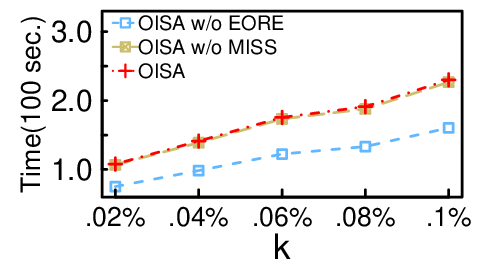
Figure 5(e) compares the running time. EA considers every possible edge and thus incurs the largest running time. BUM requires the least running time since it only retrieves the nodes with the largest LCC as the terminals of the intervention edges. OISA needs slightly more time but obtains much better solutions since it carefully examines multiple anticipated LCCs, i.e., . Also, OISA takes a longer time on Flickr since Flickr has much more large-LCC nodes, and it is necessary for OISA to derive the optionality for all these nodes. The running time of EA and TEA grows significantly on Flickr than on CPEP, as EA, TEA and GD need to examine every candidate edge not in , and CPEP is denser than Flickr. Figure 5(f) shows that the average closeness of targeted nodes in various . Be noted that the average betweenness of targeted nodes has a similar trend with Figure 5(f) and thus eliminated here. The difference between OISA and baselines is similar to the case of NILD-S.
Next, we conduct a sensitivity test on the average LCC of networks and show the component effectiveness. The results on CPEP and Facebook are similar to those of Flickr and thus not shown here.
Varying average LCC. We evaluate OISA on Youtube (average LCC 0.08), Amazon (average LCC 0.40), and Cond-Mat (average LCC 0.63) with of the number of edges in each network, i.e., for Youtube, for Amazon, and for Cond-Mat. Figure 5(g) shows that the maximum LCC is larger when the average LCC of the dataset grows, and OISA outperforms other baselines.
6.3. Empirical Study
The empirical study aims at evaluating the utility and feasibility of the proposed network intervention algorithm in real-world settings. The study, spanned over two months, included 8 weekly measurements of psychological outcomes among 424 participants, aged between 18 and 25. The participants were university students and employees with 638 pre-existing friendship links at the beginning of the study. Four self-reported standard psychological questionnaires were adopted as indicators, including Beck Anxiety Inventory (BAI) (Beck et al. 1988) for anxiety, Perceived Stress Scale (PSS) (Cohen 1994) for stress, Positive And Negative Affect Schedule (PANAS) (Watson et al. 1988) for emotion, and Psychological well-being Scale (PWS) (Stanford SPARQ 2018) for well-being. Table 3 summarizes some evaluated items in the above questionnaires. In PANAS, there are 12 positive emotion terms and 14 negative emotion terms, and the overall score is the total score of 12 positive emotion terms minus the total score of negative emotion terms. For anxiety and stress, higher scores indicate higher levels of anxiety and perceived stress, respectively. For emotion and well-being, higher scores imply better emotion and psychological well-being.
| Questionnaire | Sampled Items |
|---|---|
| BAI (anxiety), 33 items with 0–3 points | • Numbness or tingling • Unable to relax • Fear of worst happening |
| PSS (Stress), 5 sampled items with 0–4 points | • In the last month, how often have you been upset because of something that happened unexpectedly? • In the last month, how often have you felt nervous and stressed? • In the last month, how often have you felt that things were going your way? |
| PANAS (emotion), 26 sampled items with 1–4 points | • Positive emotions: excited, happy, satisfied, calm, relaxed, interested, proud, lively, love, determined, attentive, active • Negative emotions: tired, depressed, sad, angry, anxious, distressed, upset, scared, irritable, ashamed, nervous, tense, hostile, afraid |
| PWS (well-being), 18 items with 1–7 points | • I like most parts of my personality. • When I look at the story of my life, I am pleased with how things have turned out so far. • Some people wander aimlessly through life, but I am not one of them. |
To evaluate the effects of adding friendship links based on different approaches, the participants were randomly assigned to one of the following four groups: three intervention groups and one control group, with 103 participants in every group.55 5 Before the study started, participants in the four groups were requested to fill the questionnaires to ensure that there were no statistically significant differences for those questionnaires between every pair of groups. Participants in the intervention groups were provided with explicit friendship recommendations suggested by OISA and other two baselines, GD and BUM, respectively. Among the five baselines, GD was chosen because it can be applied to propagate health-related information to prevent obesity (Wilder et al. 2018). BUM was chosen because it performs the best among all baselines in Section 6.2. In the study, was set as 28 for OISA, GD, and BUM, whereas , , , and for OISA. For OISA, GD, and BUM, the recommended edges were suggested by providing specific instructions for the participants to engage in online chatting. In contrast, participants in the control group received no intervention and explicit instruction to interact with other participants. Each participant was required to provide responses to the four questionnaires every week for a total of eight times in this study.
An important question in the study is whether the participants accepted the friendship recommendations or not. To answer this question, participants were also asked the following questions at the end of the study:
Q1. Do you feel happy chatting with this recommended participant?
Q2. After the study ends, are you willing to chat with this participant?
Q3. If possible, are you willing to become a friend of this participant?
For Q1, 80.2% of the participants reported that they felt happy during the chat with the recommended participants. For Q2, 79.9% of the participants replied that they would be willing to chat with the recommended participants even after the study ended. For Q3, 83.9% of the participants reported that they would be willing to become a friend of the recommenced participant. Accordingly, participants in this study tended to accept the friend recommendations.


To evaluate the effects of the intervention, Figure 6 reports the average improvement on each psychological outcome for GD, BUM and OISA. As shown in Figure 6(a), among three intervention groups, OISA outperforms GD and BUM in all four measures, anxiety, stress, emotion, and well-being. Figures 6(b)-(c) further divide participants into four sub-groups according to the percentage of reduction in LCC.66 6 Results of pressure, and well-being are similar and thus not shown here. Figures 6(b)-(c) manifest that greater percentages of reduction in LCC are associated with more significant improvements in the psychological outcomes. It validates that new friendships via OISA is able to improve the psychological outcomes in this study. GD is inferior due to a different goal (i.e., maximizing the social influence score). Figures 6(d)-(e) plot the average scores of anxiety and emotion of participants in the intervention groups of GD, BUM, and OISA over time. As shown in Figures 6(d)-(e), the improvements of OISA is the most significant. In contrast, GD and BUM do not consider multiple network characteristics simultaneously. Figure 6(f), which plots the improvement of OISA for each outcome, also manifests that the improvements on anxiety, stress, and emotion with negative feelings are slightly better than that on well-being with only positive feelings, because brains tend to focus on potential threatening and negative emotions (Kensinger 2007). In this case, the friend candidate recommended by OISA is able to provide social support to the participants.
We also evaluate OISA, GD and BUM separately with mixed effects modeling (Jaeger 2008), a statistical technique to examine if the intervention group and control group are statistically different. Specifically, we fitted the model:
| (5) | ||||
where represents participant ’s emotion at time ; denotes whether participant is in the control group () or the intervention group (); represents the number of weeks elapsed since the study started. The study starts at time 0. is a group intercept term representing the predicted outcome for the control group at time 0. is the participant ’s deviation in intercept relative to , which is a random effect in intercept at time 0. — are the regression weights associated with , and their interaction, respectively. Specifically, indicates the difference in predicted psychological outcomes between the control group and intervention group at time 0; represents the estimated amount of change in emotion in the control group for each week of elapsed time (i.e., the “placebo effect”, or the improvements in psychological outcomes shown by the control group). Finally, is the most important, i.e., the regression coefficient for the interaction reveals the estimated difference in the amount of change in outcomes reported by the intervention group relative to the control group for each week of elapsed time. If is statistically significantly different from 0, OISA (or other baselines) is able to change the participants’ health outcomes with time substantially more than what is expected in the control group. Finally, represents the residual error in the negative emotion that cannot be accounted for by other terms.
Table 4 presents the results of model fitting of OISA. Estimates with -values smaller than 0.05 are identified as statistically significantly different from 0. Thus, the two values of , the predicted psychological outcomes of the control group at time 0, are estimated to be significantly different from 0. The term is not significantly different from 0 for all the four outcomes, which validates our random assignment procedure — indicating that the intervention and control group do not differ substantially in their anxiety, stress, emotion and well-being scores at time 0. Also, the control group does not show substantial changes in all the four outcomes with time, as is not significant. Moreover, the values of are negative and significantly different from zero for anxiety and stress, indicating that the intervention group shows statistically greater decreases in anxiety and stress. Similarly, the values of are positive and significantly different from zero for emotion and well-being, indicating that the intervention group shows statistically greater increase in emotion and well-being. In other words, the intervention group, whose friendship recommendation is suggested by OISA, shows statistically greater improvement for all the four outcomes. Also, the more extreme test statistic value (-value) and its corresponding -value, associated with the outcomes, suggest that the intervention have a more systematic effect (i.e., less uncertainty or smaller standard error) (Casella and Berger 2002). Also, Table 5 and Table 6 reveal that the model fitting results for BUM and GD are not statistically significant.
| Estimates |
|
df | -values | -values | |||
| Anxiety | 13.64 | 1.17 | 320.64 | 11.70 | <0.0001*** | ||
| -0.69 | 1.65 | 323.10 | -0.42 | 0.6763 | |||
| -0.09 | 0.15 | 1082.86 | -0.59 | 0.5532 | |||
| -0.61 | 0.21 | 1085.94 | -2.97 | 0.0030** | |||
| Stress | 14.84 | 0.32 | 364.78 | 46.02 | <0.0001*** | ||
| 0.76 | 0.46 | 367.97 | 1.66 | 0.0982 | |||
| 0.07 | 0.04 | 1083.49 | 1.56 | 0.1187 | |||
| -0.19 | 0.06 | 1087.00 | -2.95 | 0.0033** | |||
| Emotion | 4.60 | 1.14 | 298.29 | 4.05 | <0.0001*** | ||
| -0.08 | 1.61 | 300.36 | -0.05 | 0.9580 | |||
| -0.25 | 0.13 | 1082.17 | -1.85 | 0.0640 | |||
| 0.96 | 0.19 | 1084.98 | 5.09 | <0.0001*** | |||
| Well-being | 74.54 | 1.07 | 241.65 | 69.73 | <0.0001*** | ||
| 0.09 | 1.51 | 242.67 | 0.06 | 0.9545 | |||
| -0.18 | 0.09 | 1081.12 | -1.95 | 0.0515 | |||
| 0.45 | 0.13 | 1082.87 | 3.41 | 0.0007*** |
| Estimates |
|
df | -values | -values | |||
| Anxiety | 13.64 | 1.29 | 293.57 | 10.61 | <0.0001*** | ||
| -0.48 | 1.88 | 307.70 | -0.26 | 0.7990 | |||
| -0.09 | 0.16 | 972.57 | -0.56 | 0.5780 | |||
| -0.29 | 0.24 | 981.08 | -1.23 | 0.2190 | |||
| Stress | 14.84 | 0.32 | 312.83 | 45.71 | <0.0001*** | ||
| 0.09 | 0.48 | 329.18 | 0.20 | 0.8440 | |||
| 0.07 | 0.04 | 973.09 | 1.66 | 0.0970 | |||
| 0.07 | 0.06 | 982.44 | 1.16 | 0.2450 | |||
| Emotion | 4.60 | 1.19 | 267.38 | 3.84 | 0.0002*** | ||
| 0.36 | 1.75 | 278.62 | 0.20 | 0.8394 | |||
| -0.25 | 0.13 | 969.85 | -1.85 | 0.0648 | |||
| 0.38 | 0.20 | 977.27 | 1.86 | 0.0638 | |||
| Well-being | 74.54 | 1.13 | 228.79 | 65.74 | <0.0001*** | ||
| -0.35 | 1.65 | 234.92 | -0.21 | 0.8322 | |||
| -0.18 | 0.10 | 970.51 | -1.86 | 0.0636 | |||
| 0.25 | 0.15 | 975.22 | 1.67 | 0.0946 |
| Estimates |
|
df | -values | -values | |||
| Anxiety | 13.63 | 1.21 | 327.22 | 11.24 | <0.0001*** | ||
| -3.08 | 1.73 | 333.55 | -1.79 | 0.0752 | |||
| -0.09 | 0.16 | 1039.23 | -0.55 | 0.5827 | |||
| -0.26 | 0.23 | 1049.23 | -1.12 | 0.2615 | |||
| Stress | 14.84 | 0.33 | 342.38 | 45.46 | <0.0001*** | ||
| 0.86 | 0.46 | 349.29 | 1.85 | 0.0654 | |||
| 0.07 | 0.04 | 1040.66 | 1.60 | 0.1105 | |||
| -0.05 | 0.06 | 1051.23 | -0.76 | 0.4454 | |||
| Emotion | 4.60 | 1.11 | 299.82 | 4.15 | <0.0001*** | ||
| 2.42 | 1.58 | 304.93 | 1.53 | 0.1262 | |||
| -0.25 | 0.13 | 1039.63 | -1.87 | 0.0613 | |||
| 0.29 | 0.19 | 1048.12 | 1.52 | 0.1291 | |||
| Well-being | 74.54 | 1.08 | 240.07 | 69.00 | <0.0001*** | ||
| 1.00 | 1.53 | 242.46 | 0.65 | 0.5161 | |||
| -0.18 | 0.09 | 1038.35 | -1.94 | 0.0529 | |||
| 0.26 | 0.14 | 1043.01 | 1.93 | 0.0537 |
Lastly, inspection of these results by 11 clinical psychologists and professors4, is carried out to observe the behavioral implications behind the scores. The psychologists and professors are asked to the following question in Likert scale: Is the network intervention help improve the participants’ outcomes? Comparing their evaluation among intervention and control groups, the results indicate that 82% of psychologists and professors agree that the recommendation of OISA is the most effective; while only 9% of them agree for GD and BUM. The above results lead to consistent conclusion with the study — the intervention is therapeutic and positive enough to be brought into clinical consideration.
7. Conclusion
Even though research has suggested the use of network intervention for improving psychological outcomes, there is no effective planning tool for practitioners to select suitable intervention edges from a large number of candidate network characteristics. In this paper, we formulate NILD-S and NILD-M to address this practical need. We prove the NP-hardness and inapproximability, and propose effective algorithms for them. Experiments based on real datasets show that our algorithms outperform other baselines in terms of both efficiency and effectiveness; empirical results further attest to the practical feasibility and utility of using the OISA algorithm for real-world intervention purposes.
Acknowledgements.
This work was supported in part by the National Science Foundation (IIS-1717084, SMA-1360205, IGE-180687, SES-1357666), the Ministry of Science and Technology (107-2221-E-001-011-MY3, 108-2221-E-001-002, 108-2636-E-007-009-), the National Institutes ofHealth (U24AA027684), the Penn State Quantitative Social Sciences Initiative, and the the National Center for Advancing Translational Sciences (UL TR000127).
Appendix A Appendices
A.1. Proof of Theorem 5
Without loss of generality, we assume that nodes are numbered in the ascending order of their weights, i.e., if . In the following, we first introduce the properties of threshold graphs regarding LCC in Corollary 1 and Lemma 2, and then discusses the feasibility of the solution returned by CRPD in Lemma 3.
Corollary 0.
Given a threshold graph with the node weights and threshold , the nodes (with ID 1, 2,…., )are separated into three sets, , , and , where is the largest node satisfying , and is the node satisfying and . Then, 1) any node has no incident edge. 2) For any two nodes and in , . 3) For any two nodes and in , .
Lemma 0.
After is added to , the LCC of every remains the same.
Proof.
We also prove the lemma by contradiction. Assume the LCC of a becomes different. Two possible cases exist. (1) is not a neighbor of and , i.e., and . (2) is the neighbor of either or . Without loss of generality, we assume but . For the first case, and are not in the subgraph induced by and the neighbors of . Thus, adding does not change ’s LCC. For the second case, is in the subgraph induced by and its neighbors, but is not. Therefore, is not included in the induced subgraph. ∎
Lemma 0.
For , if there exists at least one feasible solution following the constraints of NILD-S on , , , and , the solution obtained by CRPD is always feasible.
Proof.
Assume that has at least one feasible solution , but the solution obtained by CRPD is different and infeasible. If there are multiple feasible solutions, let be the one with the most common nodes with . Let and denote the first different node in and when all nodes are sorted according to their IDs in the threshold graph, respectively. Note that the ID of is smaller than ; otherwise CRPD would choose in . In the following, we prove that connecting to the nodes in leads to another feasible solution following the constraints on , , and . 1) Both and add new neighbors to , and the degree of for always exceeds . 2) The betweenness of is the proportion of shortest paths among all node pairs passing through . If both and are in , the betweenness of is the same in and , because the length of shortest paths among all nodes in is at most 2, and the betweenness will not be improved by edges in or . If both and are in , the betweenness of is the same, because the number of node pairs with and the corresponding shortest paths not passing through after removing is identical to the number of node pairs with and the corresponding shortest paths passing through after adding . If and , the betweenness of grows and becomes larger than , because the shortest paths of node pairs with pass through . Therefore, the betweenness of in solution is larger than . 3) The closeness of is the sum of reciprocal of distances to other nodes. If both and are in (or both and are in ), the closeness of is the same. If and , the closeness of increases because the distance between and changes from 1 to 3, but the distance between and changes from to 1. ∎
Theorem 5 proves that the above feasible solution is optimal.
Theorem 2.
The CRPD algorithm can find the optimal solution of NILD-S when is a threshold graph, and the running time of CRPD is .
Proof.
We prove the optimality by exploring the following two cases: 1) and 2) . For the first case, according to Definition 4, a node with a larger weight is more inclined to connect to others. According to Corollary 1, forms an independent set. Also, the nodes are ordered in the ascending order of the degrees. Thus, CRPD examines nodes in the ascending order of their weights and chooses all nodes in . Adding edges in will optimize the LCC of because of the following reasons. (a) Adding edges in only changes the LCCs of the nodes in according to Lemma 2. (b) For the nodes in , its degree is increased by 1 (i.e, connecting to ), but the LCC remains as 0 because is an independent set. (c) The LCCs of nodes in is 1, and the LCCs of nodes in are impossible to be increased. (d) The LCC of will be optimized because adding edges in only increases the denominator in Equation 1, but it does not increase the numerator in Equation 1. Thus, if , CRPD finds the optimal solution.
Next, we prove the second case by contradiction. Assume that there is an optimal solution better than the solution obtained by CRPD. When there are multiple optimal solutions, let be the one such that has the most common nodes with . Let and , such that and are the first different node in and when all nodes are sorted according to their IDs. is smaller than ; otherwise CRPD would select in . Moreover, according to Definition 4. We consider another solution with . First, the solution is a feasible solution due to the following reason. If , the LCC of after adding satisfies the LCC degradation constraint since the LCC of is 1 before adding edges (i.e., never increase), and the LCC of remains as 0 before and after adding edges. On the other hand, if , the LCC of after adding is identical to the one after adding , because all nodes and are fully connected, and the number of edges between ’s neighbors is thereby the same. Second, the LCC of after adding is not larger than the LCC of in solution , as . Thus, it contradicts that is the optimal solution with the most common nodes with .
In LCC Calculation Step, to find the number of edges between node neighbors, CRPD stores a count for each node. For each edge , it examines the neighbors of the terminal nodes and in time, where is the maximum degree in . For every common neighbor of and , CRPD increases its count by 1. After examining all edges in time, CRPD extracts for each node . (2) With , CRPD finds of every node in in time, and the total time complexity in LCC Calculation Step is . In Edge Selection Process Step, CRPD first examines each of ’s two-hop neighbors and excludes if adding increases the LCC of any ’s one-hop neighbor to more than in time. Then, CRPD acquires an initial solution in iterations. In each iteration, CRPD first finds from the remaining candidates in time and excludes any node if adding will increase another node’s LCC to more than in time. The total time to find the initial solution is . After that, CRPD explores another solution starting from in time. In summary, CRPD requires in LCC Calculation Step and in Edge Selection Processing Step, and the total running time is .77 7 We follow existing algorithms to obtain the betweenness and closeness in an incremental manner, and the worst-case time complexity is to update the betweenness and closeness of all nodes after adding an edge (Kas et al. 2013b; Kas et al. 2013a). ∎
A.2. Proof of Lemma 2
We prove the lemma by contradiction. Assume there exists a such that the LCC of the node can be reduced to with only edges. First, the LCC of becomes after edges are added and connected to , where is the number of edges between ’s original neighbors before adding the new edges (i.e., ), and is the number of edges between the original neighbors and the new neighbors or between any two new neighbors. Thus, it leads to a contradiction because
| (6) | ||||
when . Note that if the LCC of is already smaller than . Therefore, is a lower bound on for while satisfying the degree constraint , since an edge connects two nodes.
A.3. Proof of Theorem 8
Before OISA starts, for every , can be derived by solving a quadratic equation in time. OISA skips an if . Otherwise, PONF iteratively 1) retrieves the largest LCC among all nodes in in time, 2) calculates the optionality of the nodes with the largest LCC to find in time (where is the number of nodes with the largest LCC), and 3) chooses the node with the largest LCC among all option nodes to extract in time. After is selected, ALC updates the LCCs in time since ALC examines the LCCs of , , and their common neighbors, and updates their LCCs if necessary. The updates for and require time, and the updates for the common neighbors take time. Thus, the total running time is , where is the number of targeted LCCs with .7
References
- [1]
- Barbieri et al. [2014] Nicola Barbieri, Francesco Bonchi, and Giuseppe Manco. 2014. Who to follow and why: link prediction with explanations. In KDD.
- Beck et al. [1988] Aaron Beck, Norman Epstein, Gary Brown, and Robert Steer. 1988. An inventory for measuring clinical anxiety: psychometric properties. Journal of consulting and clinical psychology 56, 6 (1988), 893.
- Berkman et al. [2000] Lisa Berkman, Thomas Glass, Ian Brissette, and Teresa Seeman. 2000. From social integration to health: Durkheim in the new millennium. Social Science & Medicine (2000).
- Brochier et al. [2019] Robin Brochier, Adrien Guille, and Julien Velcin. 2019. Link Prediction with Mutual Attention for Text-Attributed Networks. In WWW. ACM, 283–284.
- Casella and Berger [2002] George Casella and Roger Berger. 2002. Statistical inference. Vol. 2. Duxbury Pacific Grove, CA.
- Chang and Locke [2016] Ya-Chih Chang and Jill Locke. 2016. A systematic review of peer-mediated interventions for children with autism spectrum disorder. Research in Autism Spectrum Disorders 27 (2016), 1–10.
- Chen et al. [2018] Hongxu Chen, Hongzhi Yin, Weiqing Wang, Hao Wang, Quoc Viet Hung Nguyen, and Xue Li. 2018. PME: projected metric embedding on heterogeneous networks for link prediction. In KDD. ACM, 1177–1186.
- Cohen [1994] Sheldon Cohen. 1994. Perceived stress scale. Measuring Stress: A Guide for Health and Social Scientists 10 (1994).
- Cohen et al. [2000] Sheldon Cohen, Lynn Underwood, and Benjamin Gottlieb. 2000. Social support measurement and intervention: A guide for health and social scientists.
- Crescenzi et al. [2016] Pierluigi Crescenzi, Gianlorenzo D’angelo, Lorenzo Severini, and Yllka Velaj. 2016. Greedily improving our own closeness centrality in a network. ACM Trans. on Knowledge Discovery from Data (2016).
- De La Haye et al. [2011] Kayla De La Haye, Garry Robins, Philip Mohr, and Carlene Wilson. 2011. How physical activity shapes, and is shaped by, adolescent friendships. Social Science & Medicine (2011).
- Dhand et al. [2016] Amar Dhand, Douglas A Luke, Catherine E Lang, and Jin-Moo Lee. 2016. Social networks and neurological illness. Nature Reviews Neurology (2016).
- Durkheim [1951] Emile Durkheim. 1951. Suicide: a study in sociology. The Free Press.
- Erickson [1984] Gerald Erickson. 1984. A framework and themes for social network intervention. Family Process (1984).
- Fu et al. [2018] Chenbo Fu, Minghao Zhao, Lu Fan, Xinyi Chen, Jinyin Chen, Zhefu Wu, Yongxiang Xia, and Qi Xuan. 2018. Link weight prediction using supervised learning methods and its application to yelp layered network. IEEE Trans. on Knowledge and Data Engineering 30, 8 (2018), 1507–1518.
- Gest et al. [2014] Scott Gest, Rebecca Madill, Kathleen Zadzora, Aaron Miller, and Philip Rodkin. 2014. Teacher management of elementary classroom social dynamics: associations with changes in student adjustment. J. of Emotional & Behavioral Disorders (2014).
- House et al. [1988] James House, Karl Landis, and Debra Umberson. 1988. Social relationships and health. Science 241, 4865 (1988), 540–545.
- Howell et al. [2014] Jennifer Howell, Namkje Koudenburg, David Loschelder, Dale Weston, Katrien Fransen, Stefano De Dominicis, Stephen Gallagher, and S. Alexander Haslam. 2014. Happy but unhealthy: The relationship between social ties and health in an emerging network. European J. of Social Psychology (2014).
- Jaeger [2008] T. Florian Jaeger. 2008. Categorical data analysis: away from ANOVAs (transformation or not) and towards logit mixed models. J. of memory and language 59, 4 (2008), 434–446.
- Kas et al. [2013a] Miray Kas, Kathleen M. Carley, and L. Richard Carley. 2013a. Incremental closeness centrality for dynamically changing social networks. In ASONAM. 1250–1258.
- Kas et al. [2013b] Miray Kas, Matthew Wachs, and L. Richard Carley, Kathleen M.and Carley. 2013b. Incremental algorithm for updating betweenness centrality in dynamically growing networks. In ASONAM. 33–40.
- Kensinger [2007] Elizabeth Kensinger. 2007. Negative emotion enhances memory accuracy: Behavioral and neuroimaging evidence. Current Directions in Psychological Science 16, 4 (2007), 213–218.
- King et al. [2006] Cheryl King, Lesli Preuss, and Anne Kramer. 2006. Youth-nominated support team for suicidal adolescents: a randomized controlled trial. J. of Consulting & Clinical Psychology (2006).
- Lee et al. [2017] Seungyoon Lee, Jeremy Foote, Zachary Wittrock, Siyu Xu, Li Niu, and Doran French. 2017. Adolescents’ perception of peer groups: psychological, behavioral, and relational determinants. Social Science Research (2017).
- Lim and Kang [2015] Yongsub Lim and U Kang. 2015. Mascot: Memory-efficient and accurate sampling for counting local triangles in graph streams. In KDD.
- Lozin and Milanič [2008] Vadim Lozin and Martin Milanič. 2008. A polynomial algorithm to find an independent set of maximum weight in a fork-free graph. J. of Discrete Algorithms (2008).
- Masuda et al. [2004] Naoki Masuda, Hiroyoshi Miwa, and Norio Konno. 2004. Analysis of scale-free networks based on a threshold graph with intrinsic vertex weights. Physical Review E 70, 3 (2004), 036124.
- McGregor et al. [2016] Andrew McGregor, Sofya Vorotnikova, and Hoa Vu. 2016. Better algorithms for counting triangles in data streams. In Proceedings of the Symposium on Principles of Database Systems. 401–411.
- Mislove et al. [2007] Alan Mislove, Massimiliano Marcon, Krishna P Gummadi, Peter Druschel, and Bobby Bhattacharjee. 2007. Measurement and analysis of online social networks. In SIGCOMM.
- Papagelis [2015] Manos Papagelis. 2015. Refining social graph connectivity via shortcut edge addition. ACM Trans. on Knowledge Discovery from Data (2015).
- Saha et al. [2016] Budhaditya Saha, Thin Nguyen, Dinh Phung, and Svetha Venkatesh. 2016. A framework for classifying online mental health-related communities with an interest in depression. IEEE J. of Biomedical and Health Informatics (2016).
- Saha et al. [2014] Sudipta Saha, Niloy Ganguly, Animesh Mukherjee, and Tyll Krueger. 2014. Intergroup networks as random threshold graphs. Physical Review E (2014).
- Scellato et al. [2014] Salvatore Scellato, Anastasios Noulas, and Cecilia Mascolo. 2014. Exploiting place features in link prediction on location-based social networks. In KDD.
- Shen et al. [2017] Chih-Ya Shen, Liang-Hao Huang, De-Nian Yang, Hong-Han Shuai, Wang-Chien Lee, and Ming-Syan Chen. 2017. On finding socially tenuous groups for online social networks. In KDD.
- Sherman et al. [2009] Susan Sherman, Catherine Sutcliffe, Bangorn Srirojn, Carl Latkin, Apinun Aramratanna, and David Celentano. 2009. Evaluation of a peer network intervention trial among young methamphetamine users in Chiang Mai, Thailand. Social Science & Medicine (2009).
- Shuai et al. [2019] Hong-Han Shuai, Yen-Chieh Lien, De-Nian Yang, Yi-Feng Lan, Wang-Chien Lee, and Philip S. Yu. 2019. Newsfeed Filtering and Dissemination for Behavioral Therapy on Social Network Addictions. In CIKM.
- Shuai et al. [2016] Hong-Han Shuai, Chih-Ya Shen, De-Nian Yang, Yi-Feng Lan, Wang-Chien Lee, Philip S Yu, and Ming-Syan Chen. 2016. Mining online social data for detecting social network mental disorders. In WWW.
- Shuai et al. [2017] Hong-Han Shuai, Chih-Ya Shen, De-Nian Yang, Yi-Feng Carol Lan, Wang-Chien Lee, S Yu Philip, and Ming-Syan Chen. 2017. A comprehensive study on social network mental disorders detection via online social media mining. Transactions on Knowledge and Data Engineering 30, 7 (2017), 1212–1225.
- SNAP [2018] SNAP. 2018. http://snap.stanford.edu/.
- Stanford SPARQ [2018]
Stanford SPARQ.
2018.
http://sparqtools.org/mobility-measure/psychological-
wellbeing-scale/. - Thoits [1983] Peggy Thoits. 1983. Multiple identities and psychological well-being: a reformulation and test of the social isolation hypothesis. American Sociological Review (1983).
- TYP [2018] TYP. 2018. http://www.typ.sinica.edu.tw/E/?q=node/6.
- Ueno [2005] Koji Ueno. 2005. The effects of friendship networks on adolescent depressive symptoms. Social Science Research (2005).
- Valente [2012] Thomas Valente. 2012. Network interventions. Science (2012).
- Van Den Oord and Van Rossem [2002] Edwin Van Den Oord and Ronan Van Rossem. 2002. Differences in first graders’ school adjustment: the role of classroom characteristics and social structure of the group. J. of School Psychology (2002).
- Vernitski and Pyatkin [2012] Alexei Vernitski and Artem Pyatkin. 2012. Astral graphs (threshold graphs), scale-free graphs and related algorithmic questions. Journal of Discrete Algorithms 12 (2012), 24–28.
- Viswanath et al. [2009] Bimal Viswanath, Alan Mislove, Meeyoung Cha, and Krishna Gummadi. 2009. On the evolution of user interaction in facebook. In WOSN.
- Wang et al. [2018] Hongwei Wang, Fuzheng Zhang, Min Hou, Xing Xie, Minyi Guo, and Qi Liu. 2018. Shine: Signed heterogeneous information network embedding for sentiment link prediction. In WSDM. ACM, 592–600.
- Watson et al. [1988] David Watson, Lee Anna Clark, and Auke Tellegen. 1988. Development and validation of brief measures of positive and negative affect: the PANAS scales. Journal of personality and social psychology 54, 6 (1988), 1063.
- Weiss [1974] Robert Weiss. 1974. The provisions of social relationships. Doing unto Others (1974).
- Wilder et al. [2018] Bryan Wilder, Han Ching Ou, Kayla de la Haye, and Milind Tambe. 2018. Optimizing network structure for preventative health. In AAMAS. 841–849.
- Yuan et al. [2017] Chien-Wen Yuan, Jessica Kropczynski, Richard Wirth, Mary Beth Rosson, and John Carroll. 2017. Investigating Older Adults’ Social Networks and Coproduction Activities for Health. In PervasiveHealth.
- Zhang and Chen [2018] Muhan Zhang and Yixin Chen. 2018. Link prediction based on graph neural networks. In NIPS. 5165–5175.